Bank Failure Prediction in the COVID-19Environment

Bank Failure Prediction in the COVID-19 Environment

Tamás Kristóf¹

Associate Professor, Corvinus University of Budapest, Hungary E-mail: tamas.kristof@uni-corvinus.hu

Received: 24 December 2020; Revised: 13 January 2020;

Accepted 27 January 2020; Publication: 10 February 2021

Abstract: The paper delivers a multi­state, continuous, non­homogeneous Markov chain to present a COVID­19 stressed probability of default (PD) model for banks. First it analyzes the theoretical and methodological considerations of bank failure. Then it provides a comprehensive review of earlier empirical bank failure models published in literature. It makes the case for a multi­state model design, which has numerous advantages over the conventional binary classification techniques. A formal description of Markov chain modeling is followed by the detailed presentation of empirical model development.

Eventually it estimates PDs for a five­year forecast horizon with the developed model reflecting COVID­19 crisis impacts.

Keywords: bank failure prediction, credit risk modeling, Markov chain, stress testing JEL classification codes: C53, G17, G32

Introduction

Failure prediction is a well­established, widely studied, extensively researched subject for theoretical and empirical studies. In particular, corporate failure has been a research focus for a long time. From methodological point of view, bank failure prediction is similar to corporate failure prediction, however, fewer data, fewer default observations and different model variables generate considerable research challenges.

The financial health of the banking industry is an important prerequisite for economic stability and growth. For banks, the COVID­19 crisis could probably result in repayment difficulties for many of their clients due to defaults, restructurings or deferred payments. Profitability and capital adequacy are anticipated to decline.

Under such circumstances, substantially growing number of bank failures can be expected compared to the normal years, which makes it necessary to prepare such a bank failure model that manages the impacts of COVID­19 crisis.

The paper delivers a multi­state, continuous, non­homogeneous Markov chain to present a COVID­19 stressed probability of default (PD) model for banks. First it analyzes the theoretical and methodological considerations of bank failure. Then it provides a comprehensive review of earlier empirical

bank failure models published in literature. It makes the case for a multi­state model design, which has numerous advantages over the conventional binary classification techniques. A formal description of Markov chain modeling is followed by the detailed presentation of empirical model development.

Eventually it estimates PDs for a five­year forecast horizon with the developed model reflecting COVID­19 crisis impacts.

Theoretical and methodological considerations

The financial health of the banking industry is an important prerequisite for economic stability and growth.Since the banking system plays an important role in a country’s economic development, a banking crisis might generate serious disruptions of a country’s economic activities. Accordingly, it can be argued that reliable bank failure prediction can diminish potential real economy problems.

Failure prediction is a well­established, widely studied, extensively researched subject for theoretical and empirical studies. In particular, corporate failure has been a research focus for a long time. One of the fundamental questions of management and organization sciences is why certain organizations survive, whereas others disappear (Kristóf and Virág 2019).

In recent decades substantial number of publications have emerged in literature in the fields of business failure, corporate survival, bankruptcy prediction, organizational mortality, financial distress, default prediction and credit scoring, which might seem to be at first glance different things; however, it is a mutual effort of them that they attempt to predict the occurrence of a failure event with the help of descriptive variables by applying similar methods (Kristóf and Virág 2020). It can be argued that bank failure is relatively neglected in literature having corporate failure dominance,despite the fact that bank defaults might generate substantially higher problems in economy and society than the default of certain companies.

From methodological point of view, bank failure prediction is similar to corporate failure prediction; however, since much less banks operate in the world than companies, it necessarily leads to fewer data, in particular fewer default observations. Model variables are also different in case of bank failure prediction because of different performance indicators. The variable­family of bank indicators applied in rating and failure prediction are widely called as CAMEL expressing Capital adequacy, Assets, Management Capability, Earnings, Liquidity and Sensitivity (Rahman and Islam 2017).

Credit risk is the risk of a loss arising from the failure of a counterparty to honor its contractual obligations (McNeil et al. 2015). It incorporates both default risk, namely the risk of losses due to the default of a borrower or a trading partner, and downgrade risk, which is the risk of losses caused by a deterioration in the credit quality of a counterparty that translates into a downgrading in a rating system.

Credit risk analysis of financial instruments is a central issue of finances from theoretical and empirical points of view. One of the most important research fields, which is at the same time the fundamental credit risk parameter of the debtors, is the PD.

In recent decades, there have been several developments in the field of credit risk modeling, from which two methodological approaches are relevant for the current topic. ‘Default’ models apply classification techniques to estimate the probability that a borrower will default; that is, the borrower will not make any more payments under the original lending agreement. In contrast, ‘multi­state’ models estimate the probability that the borrower’s credit quality will change, including a change to default status. Accordingly, PD can be quantified both from average PDs mapped to rating classes, or by using statistical PD estimation models.

When selecting the proper model to estimate PD, an important element is the horizon over which credit losses are measured. As an industrial standard, PD models have traditionally been elaborated using cross sectional or some years of historical data, applying multivariate statistical classification methods, estimating PD mostly for one­year horizon. It has a rich literature and empirical results (see inter alia Virág and Fiáth 2010; Nyitrai and Virág 2017; Kristóf and Virág 2019; Nyitrai 2019; Nyitrai and Virág 2019; Kristóf and Virág 2020).

Since the introduction of International Financial Reporting Standards (IFRS)­9, emphasis has been laid on the timely recognition of credit losses.

The forward­looking impairment model of IFRS­9 has called for the quantification of lifetime credit losses, if significant credit risk deterioration happens to the debtors, which gave impetus to develop the methodology and practice of lifetime PD modeling (Kristóf and Virág 2017).

COVID­19 pandemic has brought new challenges to accomplish lifetime PD modeling in a forward­looking way. It is generally true that crisis brings uncertainty and negative impact on making financial forecasts (Jáki 2013a;

Jáki 2013b).

For banks, the COVID­19 crisis could probably result in repayment difficulties for many of their clients due to defaults, restructurings or deferred payments. As a result, non­performing loans and risk­weighted assets are expected to rise. Risk aversion is likely to increase, resulting in more selective financing. Profitability and capital adequacy are anticipated to decline.

Under such circumstances,substantially growing number of bank failures can be expected compared to the normal years, which makes it necessary to prepare such a bank failure model that manages the impacts of COVID­19 crisis.

Bank failure prediction models in literature

Most publications in literature are oriented to research bank failure as a negative phenomenon with focus on the events that precede their happening.

In majority of cases, multivariate classification methods are applied to classify banks into two groups discriminating the sound healthy banks from those that are in difficulties (Zaghdoudi 2013).

The initial bank failure models were based on static, one­period Multivariate Discriminant Analysis (MDA) and Logistic Regression (logit).The first MDA bank failure model was published by Sinkey (1975), and the first logit model by Martin (1977). For a comprehensive review of this period see Dimitras et al. (1996).

In the 1980s static models were more and more replaced by multi­period models, and multi­period logit models became dominant in bank failure prediction (Shumway 2001). Thomson (1991) extensively researched bank failures using such approach that took place in the United States (US) during the 1980s.

It was realized in the 1990s that bank failure models needed to be slightly different for emerging markets compared to developed banking industries.

González­Hermosillo et al. (1996) examined bank failures in Latin America by using two­step survival or hazard analysis and duration models, and developed different models for Latin American and US banks. Survival analysis has become a popular method in bank failure prediction afterwards.

The Asian crisis of 1997 brought calls to strengthen the monitoring of financial markets. Montgomery et al. (2005) investigated the causes of bank failures in Japan and Indonesia, and developed a logit model to demonstrate the usefulness of domestic bank failure prediction models through a cross­

country model that allowed for cross­correlation of the error terms.

Since the 1990s a great number of publications has recommended that machine learning techniques perform more effectively than traditional statistical techniques. Among machine­learning techniques, Artificial Neural Network (ANN) and Support Vector Machine (SVM) have appeared to be the most preferred tools in bank failure prediction.Tam and Kiang (1992) were the first to apply ANNs to bank failure prediction and found that ANNs outperformed any other earlier applied method. Since then several studies have compared ANNs and statistical techniques to predict bank failure.

Kolari et al. (2002) developed an early warning system based on logit and non­parametric Trait Recognition (TR) model for large US banks. Boyacioglu et al. (2009) examined ANN, SVM and multivariate statistical methods to predict the failure of Turkish banks. Result proved that the SVM achieved the best accuracy.

The standard two­state prediction models were later extended into three states (operational, at­risk and default) to achieve better prediction accuracy (Halling and Hayden 2007).

Reboredo (2002) published the first Markov chain model for a probabilistic evaluation of Spanish bank solvency that included heterogeneity and past solvency. Bank solvency positions were obtained from the values of a stochastic

recursive profit function. A year later Glennon and Golan (2003) developed an early­warning bank failure model designed specifically to capture the dynamic process underlying the transition from financially sound to closure. The authors modeled the transition process as a stationary Markov model and based on US chartered bank data estimated the transition probabilities using a Generalized Maximum Entropy (GME) estimation technique.

Kumar and Ravi (2007) published a comprehensive review of the application of statistical and intelligent techniques to solve the bankruptcy prediction problem faced by banks and firms starting from the appearance of the first MDA models until 2005. The review was categorized by taking the type of technique applied to solve the failure prediction problem as an important dimension.

Poghosyan and Cihák (2009) carried out a research in European Union (EU) with financial data from the period of 1997­2007. Beyond the relevance of the accustomed predictors, based on several logit models, it was concluded that contagion effects were important when predicting EU bank failures, which means that the PD of a bank is higher if there is a recent failure in a bank with similar size in the same country.

After the outbreak of the previous financial crisis a great number of publications have applied the earlier analyzed techniques to more recent data on bank failures during the financial crisis. Interesting conclusions were drawn regarding the reasons for bank failure that not much changed compared to earlier findings. Cole and White (2012) applied a standard early warning model approach to 263 US banks that either failed or were technically insolvent in 2009, and concluded that the basic drivers of bank financial performance and failure during the financial crisiswere similar to the drivers of bank performance and failure during earlier industry downturns. Fahlenbrach et al. (2012) arrived at similar conclusions. Wang and Cox (2013) examined why commercial banks in the US failed in the recent financial crisis from the aspect of risk taking by the financial institutions.

Wang et al. (2016) developed a self­organizing neural fuzzy inference system to predict bank failure using the experience of 3635 US banks over a 21­year period. The experimental results of the model were encouraging in terms of both accuracy and interpretability when benchmarked against other prediction models.

Tanaka et al. (2016) developed a Random Forest­based early warning system for predicting bank failures. Bank­level financial statements were analyzed to find patterns that identify banks in danger of failing. Experimental results showed that Random Forests outperformed conventional methods.

Cox et al. (2017) employed the Cox proportional hazards model to forecast US bank failures during the financial crisis period of 2008 to 2010. The study provided a great contribution in enduring bank attributes that can reduce the likelihood of failure.

Le and Viviani (2018) compared the accuracy of traditional statistical and machine learning techniques to predict the failure of banks using a sample of 3000 US banks. The empirical result revealed that ANNs and k­nearest neighbor (KNN)were the most reliable methods to predict bank failure.

Audrino et al. (2019) applied a generalized logit model together with mixed­

data sampling to improve the accuracy in predicting US bank failures.

Applying the model on data from the period of 2004­2016 substantially better result was achieved compared to the accuracy of classic logit model, in particular for long­term forecasting horizons.

Shrivastava et al. (2020) created a machine learning based bank failure model for Indian banks using data from 2000­2017. To handle the problem of low number of failed banks, the Synthetic Minority Oversampling Technique (SMOTE) was used. Redundant features were reduced by Lasso regression.

To avoid bias and overfitting, Random Forest and Ada Boost techniques were applied and compared to the logit to get the best predictive model.

Manthoulis et al. (2020) explored the predictive power of attributes of US banks that described the diversification of banking operations, considered the prediction of failure in a multi­period context, and introduced an enhanced ordinal classification framework (multiple criteria decision analysis, statistics, machine learning and ensemble methods). Results proved that both diversification attributes and ordinal classification provided better prediction.

After studying various literature and empirical models, the multi­state Markov chain approach was selected to develop a COVID­19 stressed lifetime PD model for banks. A multi­state model design has the advantage over the conventional binary classification techniques that it can capture the failure phases of transition process over several states, and it is also more efficient to prepare long­term forecast. The formal description of the method is provided in the following chapter.

Markov chain modeling

Markov processes are named after a Russian mathematician, Andrey Andreyevich Markov, who dealt with stochastic processes in the early 20th century (Siekelova et al. 2019). Modern probability theory studies chance processes for which the knowledge of previous outcomes influences predictions for future experiments (Spahn 2017). In the Markov process, the result of the current experiment affects the result of the experiment in the future.

According to our best knowledge, Cyert et al. (1962) published the first Markov chain­based failure model for accounts receivables. Consideration behind the application of discrete Markov chain was the fact that accounts receivables month by month migrated among different delinquency states. Movements among delinquency states were described by transition matrices.

The study of Jarrow et al. (1997) represented a milestone in literature that elaborated a continuous Markov chain model for corporate bonds, taking into account the credit rating. Changes of credit rating formulated the states of the Markov chain. The transition matrix expressed the probability of remaining in the existing rating class, and the migration to other rating classes.

Within the framework of a comparative analysis, Lando and Skodeberg (2002) compared the performance of the continuous multi­state Markov model to the traditional, cross sectional, discrete Markov model. The authors concluded that the continuous model outperformed the discrete model. Since generator matrix construction is a key issue in developing continuous Markov models, several publications have dealt with the optimization problem of the matrix logarithm (Zhang 2019).

A problem of applying Markov chain in practice emerged from the observation that the behavior of data modeled by Markov chain is often non­

homogeneous. Bluhm and Overbeck (2007) generated PD term structures using homogeneous and non­homogeneous, continuous Markov chains, and compared the results to the fifteen years of cumulated actual default rates published by Standard&Poors. Results with the non­homogeneous model were much better, from which it was concluded that the homogeneity assumption could be set aside.

A series of random variables formulate a Markov chain, if an observation is in any period in an initial i­th state, and the probability that it migrates to a j­th state in the next period, exclusively depends on the value of i. Let

denote the series of random variables with {1, 2, …, K} fixed number of classes, where K denotes the default state. The series is a finite first order Markov chain, if:

P(X_t+1 = j|X₀ = x₀, ..., X_t–1 = x_t–1, X_t = i) = P(X_t+1 = j|X_t = i) (1) for each t, and i, j�{1, 2, …, K}

P_t (i, j) = P(X_{t +1} = j|X_t = i) means the probability of transition in t­th period from i­th state to j­th state in (t+1)­th period, and represent the element of the K×K size P_t transition matrix.

The Markov chain is stationary, if P_t = P for each t � 0. Then the transition matrices are identical in each time. In this case, any multi­period transition matrix can be calculated by raising the annual transition matrix to power:

P(X_t+k = j|X_t = i) = P^k(i, j) (2) The continuous X_t Markov chain is timely homogeneous, if for each i, j state and t, s � 0 times:

P(X_t+s = j|X_t = i) = P(X_s = j|X₀ = i) (3) In case of continuous Markov chain, a transition matrix between 0­th and t­th period can be estimated by exponentiating the generator matrix. G generator matrix is such a K×K matrix, where:

P(0, t) = exp(Gt) (4) The generator matrix has the following characteristics:

• G_i,j = 0 for each i � j

• G_i,i = –�_j�i G_i,j

The elements of the generator matrix relate to the time spent in each rating class. The remaining time in i­th class can be characterized by exponential distribution having –G_i,i parameter. Timely homogeneous probabilities of transitions in any horizon can be expressed in the function of the same generator matrix. However, in case of non­homogeneous transitions, the generator matrix depends on time, and can be formulated as follows:

(0, ) exp 0^t ( )

P t G t dt (5)

Idiosyncrasies of continuous, non­homogeneous Markov chain enable the flexible interpolation of parameters, even when the research challenge is how to estimate stressed lifetime PDs amid COVID­19 circumstances by a Markov chain starting from a long­run historical average transition matrix.

Empirical research

In Markov chain modeling the first research task is to construct a transition matrix based on observed changes of states. In case of credit risk modeling it generally means an annual transition matrix, reflecting the change in rating.

For the purposes of the current research, the transition matrix of Standard &

Poors (S&P) was applied. S & P maintains a rich historical database containing the rating changes, defaults and recoveries of global financial services issuers rated by S&P. Within global financial services issuers S&P defines banks as bank holding companies, bank subsidiaries, savings and loans, credit unions and government­related entities (S & P 2019). At the time of writing this paper, the most recent transition matrix for banks has been available for the period of 1981­2018.

Table 1: Global average annual transition rates for banks (1981­2018)

AAA AA A BBB BB B CCC/C Not rated Defaulted

AAA 82.99% 10.79% 0.83% 0.21% 0.21% 0.00% 0.00% 4.98% 0.00%

AA 0.26% 86.46% 9.06% 0.37% 0.00% 0.00% 0.00% 3.85% 0.00%

A 0.03% 2.13% 87.63% 4.55% 0.25% 0.05% 0.00% 5.31% 0.04%

BBB 0.00% 0.28% 4.33% 83.69% 3.93% 0.43% 0.02% 7.16% 0.16%

BB 0.00% 0.13% 0.09% 6.40% 75.94% 5.74% 0.67% 10.40% 0.62%

B 0.00% 0.00% 0.06% 0.24% 7.16% 78.34% 2.61% 8.80% 2.79%

CCC/C 0.00% 0.00% 0.00% 0.00% 0.86% 21.46% 49.36% 16.31% 12.02%

Not rated 0.00% 0.00% 0.00% 0.00% 0.00% 0.00% 0.00% 0.00% 0.00%

Defaulted0.00% 0.00% 0.00% 0.00% 0.00% 0.00% 0.00% 0.00% 100.00%

Source: S&P (2019), p. 41

For further calculations it is necessary to handle the problem of withdrawn rating (‘Not rated’ in case of S&P). Assuming that withdrawn rating does not mean upgrading or downgrading, the matrix has been normalized by simple scaling. The sum of total rows are 100% in each line.

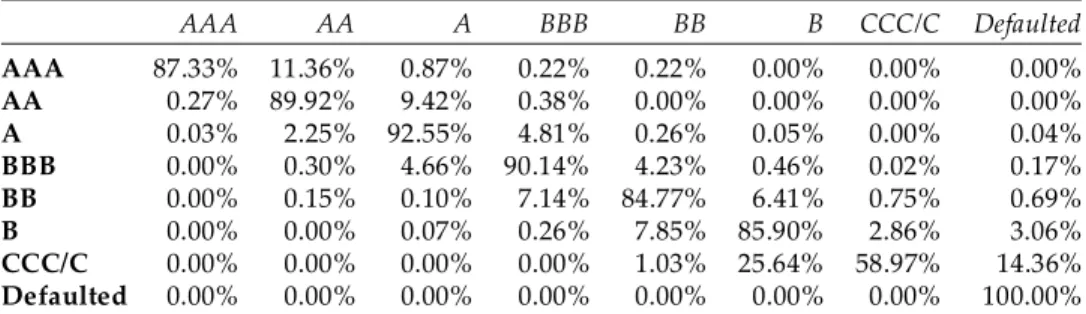
Table 2: The normalized transition matrix

AAA AA A BBB BB B CCC/C Defaulted

AAA 87.33% 11.36% 0.87% 0.22% 0.22% 0.00% 0.00% 0.00%

AA 0.27% 89.92% 9.42% 0.38% 0.00% 0.00% 0.00% 0.00%

A 0.03% 2.25% 92.55% 4.81% 0.26% 0.05% 0.00% 0.04%

BBB 0.00% 0.30% 4.66% 90.14% 4.23% 0.46% 0.02% 0.17%

BB 0.00% 0.15% 0.10% 7.14% 84.77% 6.41% 0.75% 0.69%

B 0.00% 0.00% 0.07% 0.26% 7.85% 85.90% 2.86% 3.06%

CCC/C 0.00% 0.00% 0.00% 0.00% 1.03% 25.64% 58.97% 14.36%

Defaulted 0.00% 0.00% 0.00% 0.00% 0.00% 0.00% 0.00% 100.00%

The PD of each rating category is reflected by the probability of transition to the defaulted rating category. If the classification of banks were already defaulted in the initial period of transition, both annual and lifetime PD of such banks are 100%. The defaulted classification is absorbing state, regardless of the fact where the migration is from.

For continuous Markov chain modeling, it is essential to construct a generator matrix. It is easy to see that neither the simple root nor the logarithm of the annual transition matrix is in itself appropriate, because the requirements of generator matrix are not necessarily met,and negative results might arise.

The empirical transition matrix might in itself possess such properties that exclude the existence of a generator matrix, and the same transition matrix might be resulted starting from more generator matrices (Israel et al. 2001).

Within the framework of this empirical research, an approximated generator matrix has been elaborated applying the regularization procedure published by Kreinin and Sidelnikova (2001) guaranteeing very good fit to the transition matrix considering Euclidean distance.

The first step of regularization is to take the natural logarithm of the annual transition matrix, which was done in R plus. Where negative values were resulted apart from the diagonal, they were substituted with zero, so an initial G matrix was received. To achieve that the generator matrix contains zero sums of rows, non­positive diagonal values and non­negative non­diagonal values, the rows of the matrix were modified considering the relative contribution of each element (Kreinin and Sidelnikova ibid.), formulating aG� matrix, the elements of which were calculated as follows:

� ¹

1

| |

| |

Nj ij

ij ij N

j ij

g g g

g (6)

The difference of the two matrices gives G� generator matrix, in which the sums of rows are zero:

ˆ �

G G G (7)

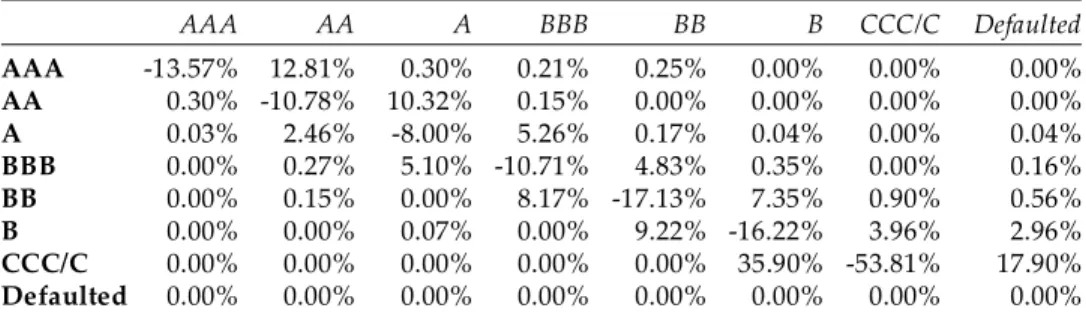
Table 3: The applied generator matrix

AAA AA A BBB BB B CCC/C Defaulted

AAA ­13.57% 12.81% 0.30% 0.21% 0.25% 0.00% 0.00% 0.00%

AA 0.30% ­10.78% 10.32% 0.15% 0.00% 0.00% 0.00% 0.00%

A 0.03% 2.46% ­8.00% 5.26% 0.17% 0.04% 0.00% 0.04%

BBB 0.00% 0.27% 5.10% ­10.71% 4.83% 0.35% 0.00% 0.16%

BB 0.00% 0.15% 0.00% 8.17% ­17.13% 7.35% 0.90% 0.56%

B 0.00% 0.00% 0.07% 0.00% 9.22% ­16.22% 3.96% 2.96%

CCC/C 0.00% 0.00% 0.00% 0.00% 0.00% 35.90% ­53.81% 17.90%

Defaulted 0.00% 0.00% 0.00% 0.00% 0.00% 0.00% 0.00% 0.00%

In line with the assumption system of the continuous Markov chain, probabilities of transitions for – even fractional – terms can be estimated, by exponentiating the generator matrix to the desired power. However, to ensure the flexibility that the estimated PD term structure well reflects the crisis situation caused by the COVID­19 pandemic, a non­homogeneous Markov chain was developed. The starting point was the ˆG generator matrix, however,, it was not assumed that the transitions were identical, and a timely dependent generator was applied:

ˆ_t ( ) ˆ

C t G (8)

where × is matrix multiplication and ( ) (t _ij( ))t 1 ,_{i j K} is such a K×K diagonal matrix, where:

,

( ) 0

ij ( )

if i j

t t if i j (9)

�_�,�(t) can be formulated in the function of non­negative � and � parameters per rating class as follows (Bluhm and Overbeck 2007):

1 ,

(1 )

( ) 1

e t t

t e (10)

In case of t = 1 the diagonal matrix purely consists of �_���(1) = 1. In the numerator (1 – e^–�t) denotes the exponential distribution of the random variable, while t^�–1 serves for convexity or concavity adjustment. Hence, both the flexibility of parameter selection and the application of well­known functions from probability theory are met. By proper selection of � and � parameters,

the generator matrix can interpolated to stressed default rates, achieving satisfactory estimation accuracy.

To optimize � and � parameters the empirical bank default rates of S&P were stressed considering the experiences from the previous financial crisis.

The long­term average annual default rates per rating classes from the period of 1981­2018 were multiplied by stress factors derived from the worst year of the previous financial crisis. Such data was available at S&P only at an aggregated level for the whole financial service sector, which is a broader category than banks.It was assumed that the crisis impact for the total financial service sector well reflected the behavior of banks.

In the AAA rating class no default event happened between 1981­2018, accordingly no stress multiplier was applied. For AA, A, BBB and BB ratings the 2008 actual default rates were related to the long­term averages, because 2008 was the worst year for these ratings in the previous financial crisis. For the same reason, the 2009 actual default rates were applied for B and CCC/C ratings. The below table summarizes the stress factors.

Table 4: The applied stress factors

Stress multiplier Method

AAA 1.000 no historical default

AA 13.875 2008 to long­term average

A 8.192 2008 to long­term average

BBB 5.500 2008 to long­term average

BB 2.209 2008 to long­term average

B 3.167 2009 to long­term average

CCC/C 1.526 2009 to long­term average

During optimization the monotonically increasing cumulated PDs, the accurate estimation of default rates, and the realistic reflection of COVID­19 effects also played important role. The nonlinear optimization was done using the Generalized Reduced Gradient (GRG) method, parameterized in such a way to achieve as accurate as possible result in the third year. The following table summarizes the so optimized parameters.

Table 5: The optimized parameters

� �

AAA 1.0673 0.8778

AA 0.8827 1.3696

A 0.7638 1.4869

BBB 0.4118 4.3784

BB 0.7580 0.8132

B 0.6670 1.1319

CCC/C 1.0906 0.5611

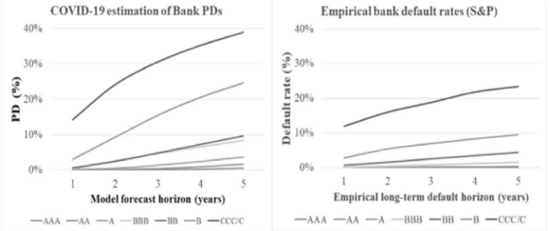
Bank PDs were estimated in a five years of forecast horizon per rating class. Results are presented in the below chart. Compared to the S&P empirical average historical default rates from the period of 1981­2018, significantly higher PDs were resulted, which is a consequence of applying the stress factors expressing the COVID­19 crisis impact.

Figure 1: Estimated PDs and empirical default rates Source: PDs – own calculations; default rates – S&P (2019)

Conclusions

The financial health of the banking industry is an important prerequisite for economic stability and growth. In particular, amid COVID­19 circumstances, reliable bank failure prediction is of growing interest.

The first bank failure prediction model was published in 1975. Since then a great development history has taken place with regard to research questions, methodological developments and empirical results. From methodological point of view, bank failure prediction is similar to corporate failure prediction;

however, fewer data, fewer default observations and different model variables generate considerable research challenges, especially when preparing such a bank failure model that can manage the impacts of COVID­19 crisis.

Within the framework of the current empirical research, a multi­state, continuous, non­homogeneous Markov chain has been developed to present a COVID­19 stressed lifetime PD model for banks. A multi­state model design has the advantage over the conventional binary classification techniques that it can capture the failure phases of transition process over several states, and it is also more efficient to prepare long­term forecast.

Bank PDs were estimated in a five years of forecast horizon per rating class. Compared to the S&P empirical average historical default rates from the period of 1981­2018, significantly higher PDs were resulted, which is a

consequence of applying the stress factors expressing the COVID­19 crisis impact.

References

Audrino, F.; Kostrov, A. & Ortega, J.­P. (2019). “Predicting U.S. bank failures with MIDAS logit models”. Journal of Financial and Quantitative Analysis, 54(6), 2575­2603.

Bluhm, C. & Overbeck, L. (2007). “Calibration of PD term structures: to be Markov or not to be”. Risk, 20(11), 98­103.

Boyacioglu, M. A.; Kara, Y. & Baykan, Ö. K. (2009). “Predicting bank financial failures using neural network, support vector machines and multivariate statistical methods: a comparative analysis in the sample of savings deposit insurance fund (SDIF) transferred banks in Turkey”. Expert Systems with Applications, 36(2), 3355­

3366.

Cole, R. A. & White, L. J. (2012). “Déjà vu all over again: The causes of U.S. commercial bank failures this time around”. Journal of Financial Services Research, 42(1), 5­29.

Cox, R. A. K.; Kimmel, R. K. &Wang, G. W. Y. (2017). “Proportional hazards model of bank failure: evidence from USA”. Journal of Economic & Financial Studies, 5(3), 35­

45.

Cyert, R.; Davidson, H. & Thompson, G. (1962). “Estimation of the allowance for doubtful accounts by Markov chains”. Management Science, 8(3), 287­303.

Dimitras, A. I., Zanakis, S. H. & Zopounidis, C. (1996). “A survey of business failure with an emphasis on prediction methods and industrial applications”. European Journal of Operational Research, 90(3), 487­513.

Fahlenbrach, R.; Prilmeier, R. & Stulz, R. M. (2012). “This time is the same: using bank performance in 1998 to explain bank performance during the recent financial crisis”.

Journal of Finance, 67(6), 2139­2185.

Glennon, D. & Golan, A. (2003). “A Markov model of bank failure estimated using an information­theoretic approach”. OCC Economics Working Paper 2003­1.

Washington: OCC

González­Hermosillo, B.; Pazarbaþioðlu, C. & Billings, R. (1996). “Banking system fragility: likelihood versus timing of failure – an application to Mexican financial crisis”. IMF Working Paper No. 96/142. Washington: International Monetary Fund Halling, M. & Hayden, E. (2007). Bank failure prediction: a three­state approach. Vienna:

Austrian National Bank

Israel, R. B.; Rosenthal, J. S. & Wie, J. Z. (2001). “Finding generators for Markov chains via empirical transition matrixes, with applications to credit ratings”. Mathematical Finance, 11(2), 245­265.

Jáki, E. (2013a). “A válság, mint negatív információ és bizonytalansági tényezõ – A válság hatása az egy részvényre jutó nyereség elõrejelzésekre”. Közgazdasági Szemle, 60(12), 1357­1369.

Jáki, E. (2013b). “Szisztematikus optimizmus a válság idején”. Vezetéstudomány, 44(10), 37­49.

Jarrow, R. A.; Lando, D. & Turnbull, S. (1997). “A Markov model for the term structure of credit risk spreads”. Review of Financial Studies, 10(2), 481­523.

Kolari, J.; Glennon, D.; Shin, H. & Caputo, M. (2002). “Predicting large US commercial bank failures”. Journal of Economics and Business, 54(4), 361­387.

Kreinin, A. & Sidelnikova, M. (2001). “Regularization algorithms for transition matrices”. Algo Research Quarterly, 4(1­2), 23­40.

Kristóf, T. & Virág, M. (2017). “Lifetime probability of default modeling for Hungarian corporate debt instruments”. In: Zoltayné Paprika, Z. et al. (Eds.): ECMS 2017: 31st European Conference on Modelling and Simulation. Nottingham: European Council for Modelling and Simulation, pp. 41­46.

Kristóf, T. & Virág, M. (2019). “A csõdelõrejelzés fejlõdéstörténete Magyarországon”.

Vezetéstudomány, 50(12), 62­73.

Kristóf, T. & Virág, M. (2020). “A comprehensive review of corporate bankruptcy prediction in Hungary”. Journal of Risk and Financial Management, 13(2), 35.

Kumar, P. R. & Ravi, V. (2007). “Bankruptcy prediction in banks and firms via statistical and intelligent techniques – a review”. European Journal of Operational Research, 180(1), 1­28.

Lando, D. & Skodeberg, T. M. (2002). “Analyzing rating transactions and rating drift with continuous observations”. Journal of Banking & Finance, 26(2­3), 423­444.

Le, H. H. &Viviani, J.­L. (2018). “Predicting bank failure: an improvement by implementing a machine­learning approach to classical financial ratios”. Research in International Business and Finance, 44(4), 16­25.

Manthoulis, G.; Doumpos, M.; Zopounidis, C. & Galariotis, E. (2020). “An ordinal classification framework for bank failure prediction: Methodology and empirical evidence for US banks”. European Journal of Operational Research, 282(2), 786­801.

Martin, D. (1977). “Early warning of bank failure: a logit regression approach”. Journal of Banking & Finance, 1(3), 249­276.

McNeil, A. J.; Frey, R. & Embrecht, P. (2015). Quantitative Risk Management. Concepts, Techniques and Tools. Princeton­Oxford: Princeton University Press

Montgomery, H.; Hahn, T. B.; Santoso, W. & Dwityapoetra, S. B. (2005). “Coordinated failure? A cross­country bank failure prediction model”. ADB Institute Discussion Paper No. 32.Manila: Asian Development Bank

Nyitrai, T. (2019). “Dynamization of bankruptcy models via indicator variables”.

Benchmarking: An International Journal, 26(1), 317­332.

Nyitrai, T. & Virág, M. (2017): “Magyar vállalkozások felszámolásának elõrejelzése pénzügyi mutatóik idõsorai alapján”. Közgazdasági Szemle, 64(3), 305­324.

Nyitrai, T. & Virág, M. (2019). “The effects of handling outliers on the performance of bankruptcy prediction models”. Socio­Economic Planning Sciences, 67(9), 34­42.

Poghosyan, T. & Èihák, M. (2009). “Distress in European banks: an analysis based on a new data set”. IMF Working Paper WP/09/9.Washington: International Monetary Fund

Rahman, Z. & Islam, S. (2017). “Use of CAMEL Rating Framework: A Comparative Performance Evaluation of Selected Bangladeshi Private Commercial Banks”.

International Journal of Economics and Finance 10(1), 120­128.

Reboredo, J. C. (2002). “Bank solvency evaluation with a Markov model”. Applied Financial Economics, 12(5), 337­345.

S&P (2019). Default, transition and recovery: 2018 annual global financial services default and rating transition study. S&P Global Ratings: www.spglobal.com/ratingsdirect Shrivastava, S.; Jevanthi, P. M. & Singh, S. (2020). “Failure prediction of Indian banks

using SMOTE, Lasso regression, bagging and boosting”. Cogent Economics &

Finance, 8(1), 1729569.

Shumway, T. (2001). “Forecasting bankruptcy more accurately: a simple hazard model”.

Journal of Business, 74(1), 101­124.

Siekelova, A.; Kovacova, M.; Lazaroiu, G. & Valaskova, K. (2019). “Prediction of payment discipline using the Markov chain – case studies of Visegrad Four”. Journal of International Studies, 12(2), 270­284.

Sinkey, J. F. (1975). “A multivariate statistical analysis of the characteristics of problem banks”. The Journal of Finance, 30(1), 21­36.

Spahn, P. (2017). “Central Bank support for government debt in a currency union”.

Journal of Self­Governance and Management Economics, 5(4), 7­34.

Tam, K. Y. & Kiang, M. Y. (1992). “Managerial applications of neural networks: the case of bank failure predictions”. Management Science, 38(7), 926­947.

Tanaka, K.; Kinkyo, T. & Hamori, S. (2016). “Random forests­based early warning system for bank failures”. Economics Letters, 148(C), 118­121.

Thomson, J. B. (1991). “Predicting bank failures in the 1980s”. Federal Reserve Bank of Cleveland Economic Review, 27(1), 9­20.

Virág, M. & Fiáth, A. (2010). Financial ratio analysis. Budapest: Aula Kiadó

Wang, G. W. Y. & Cox, R. A. K. (2013). “Risk taking by US banks led to their failures”.

International Journal of Financial Services Management, 6(1), 39­59.

Wang, D.;Quek, C.& See, N. G. (2016). “Bank failure prediction using an accurate and interpretable neural fuzzy inference system”. AI Communications, 29(4), 477­495.

Zaghdoudi, T. (2013). “Bank failure prediction with logistic regression”. International Journal of Economics and Financial Issues, 3(2), 537­543.

Zhang, L. (2019). “Convex quadratic optimization based on generator matrix in credit risk transfer process”. International Journal of Mathematics Trends and Technology, 65(3), 92­106.