Visualization of univariate data for comparison

(1)

Visualization of univariate data for comparison

Csaba Faragó

Department of Software Engineering University of Szeged, Hungary

farago@inf.u-szeged.hu

Submitted October 20, 2015 — Accepted December 07, 2015

Abstract

“A picture is worth a thousand words.” This idiom is true for research studies as well: illustrations in a paper helps the reader to better understand the findings of the authors. There are already several possibilities for visualizing data. But there always exist cases when the currently available diagram types are not useful enough. We also ran into such a situation, and created two new diagram types: Cumulative Characteristic Diagram and Quantile Difference Diagram for illustrating data sets of numeric types.

The Cumulative Characteristic Diagram is a curve, which is based on the non-ascending order of the values. It makes it easy to read many characteristics of the input data, and it is suitable to find similarities and differences between several data sets quickly.

Quantile Difference Diagram draws the differences of two ascending sets of data on the same quantiles. This diagram is suitable to illustrate in which subset the data are higher, and it also reveals some important details, which would remain hidden using statistic tests only.

We found them very useful both in explaining our actual results, and gaining ideas for further development directions. In this article we show the usefulness of these diagrams illustrating the results of Contingency Chi- Squared tests, Wilcoxon rank tests and variance tests.

Keywords: univariate data, data visualization, maintainability, Cumulative Characteristic Diagram, Quantile Difference Diagram

45(2015) pp. 39–53

http://ami.ektf.hu

39

(2)

1. Introduction

1.1. Overview

In research data arise. Visualization of this is very important, as a diagram may reveal important characteristics. Furthermore, illustrating the statistic tests with proper diagrams might help understanding the results.

A great number of diagram types exist, but sometimes none of them are really adequate for visualization. In this study we present 2 diagram types invented and implemented by us. One of them we call Cumulative Characteristic Diagram, and abbreviate CCD. The other one we call Quantile Difference Diagram, and abbreviate QDD.

These diagrams helped us in further research, and we found them useful in illustrating the results of Contingency Chi-Squared test, the Wilcoxon test and variance test.

1.2. Motivation

The motivating examples come from our research in finding the impact of various developer interactions on software quality. In this section we explain the idea using a very high level of abstraction, concentrating on the data only.

We collected sets of numbers, and divided them according to some rules to disjoint subsets. Using some statistical tests we found that there are differences among the data in the disjoint subsets, and we revealed similar patters among several executions. However, by visualizing the data with the plain old box plots or other traditional diagram types, the statistical results could not be really supported.

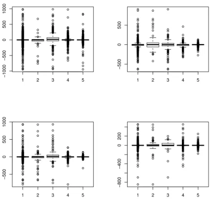
The box plots, which we found not to be useful in our special case are shown in Figure 1. Note that this version does not contain the outliers; the diagrams with outliers were even worse. On the diagram the leftmost box plot illustrates all the data, and the rest four represents the data falling into disjoint subsets. The data division was performed on four input data sets.

Based on this example we framed the Cumulative Characteristic Diagram, which proved to be suitable for illustrating the results. Furthermore, this diagram type helped us to identify additional connections not discovered earlier. The analysis of these earlier unrevealed findings leads us to framing the Quantile Difference Diagrams.

2. Related work

Several diagram types exists for illustrating univariate, bivariate and multivariate data. One of the fundamental works in this topic is the book Graphical Methods for Data Analysis (Chambers et al. [1]). For statistical package R a recommended reading is theR Graphics (Murrel [2]).

(3)

1 2 3 4 5

−1000−50005001000

1 2 3 4 5

−5000500

1 2 3 4 5

−50005001000

1 2 3 4 5

−800−4000200

Figure 1: Illustrating case: Plots with limited usefulness

The articleVariations of Box Plots by McGill et al. [3] suggests two extensions of the base box plots. Those times the computers were expensive and slow, and the diagrams were mostly drawn by hand. The study Opening the Box of a Boxplot by Benjamini [4] exploits the capability of the computer. The article Some Im- plementations of the Boxplot by Frigge et al. [5] deals mainly with the problem of outliers. The studyMethods for Presenting Statistical Information: The Box Plot by Potter et al. [6] provides a summary of the variations of box plots.

Probably the most important problem with box plot is that it hides the local densities. The mentioned studies mostly deal with this problem. To overcome this shortcoming, in R the density plot could be a good choice in several cases (using density() function fromstat, like follows: plot(density(x))). Other popular diagram types handling this issue are violin plots (R functionvioplot()in pack- agevioplot(see paperViolin Plots: a Box Plot-density Trace Synergismby Hintze and Nelson [7])) and bean plots (R functionbeanplot()in packagebeanplot, as described in paperBeanplot: A Boxplot Alternative for Visual Comparison of Dis- tributions by Kampstra [8]).

The problem of illustrating bivariate data is also very common. An early pro- posal of a bivariate extension of boxplots is presented in articleBivariate Extensions of the Boxplot by Goldberg and Iglewicz [9]. An interesting two dimensional exten-

(4)

sion of the box plots is the bag plot, suggested by articleThe Bagplot: a Bivariate Boxplot by Rousseeuw et al. [10]; R functionbagplot()in packageaplpack.

Visualizing multivariate data is even harder. ArticleThe strucplot Framework:

Visualizing Multi-way Contingency Tables with vcd by Hornik et al. [11] suggests a framework for visualizing multi-way contingency tables.

The presented R functions are mainly based on base package graphics. An- other basic visualization related package in R is grid. The lattice package is based on grid, see work Lattice: Multivariate Data Visualization with R by Sarkar [12] for details.

3. Diagrams

3.1. Cumulative Characteristic Diagram (CCD)

The input of the base diagram is a set of numbers. In the first step, these numbers are sorted non-ascending. Then cumulatives are calculated for every element: the series starts with 0, the next element will be the value of the first element of the sorted array, the second element will be the sum of the first 2 elements, and so on. In the diagrams the x coordinate represents the number of elements, and the y coordinate represents the calculated cumulatives. Instead of drawing each point one by one, these points are connected with straight lines. If the number of elements is high enough, the result will look like a continuous line without bends.

The diagram type is mostly suitable for data of normal distribution with the mean close to 0. The diagram is applicable for quick comparison of several data sets: to illustrate the similarities and differences. It can be used to illustrate quickly two or more – seemingly similar – data sets if they are really similar or not. A CCD which contains two or more characteristics on the same diagram we callComposite Cumulative Characteristic Diagram.

Examples are shown later in this chapter in Figure 2.

3.2. Quantile Difference Diagram (QDD)

The idea behind the Quantile Difference Diagrams is to compare the same quantiles of two sets of numbers. This means the first element of the first set should be compared to the first element of the second one, similarly the 10% to the 10%, the median to the medial, the 90% to the 90%, highest to the highest and so on.

Therefore the input of the QDD is always two sets of numbers. Every centile is determined in both subsets, i.e. the 0% (which is the lowest one), the 1% (e.g. if the set contains 1000 elements, this is the 10^th) etc. This results 101 values in every case, either by omitting values, or taking the same values several times. Then the differences are calculated at every centile. On the the diagram these differences are displayed as a line. Examples for QDD can be found later in this chapter in Figure 3.

(5)

3.3. The vudc R package

Both diagram types have been implemented as an R package [13], named vudc, which stand for Visualization of Univariate Data for Comparison. This can be installed directly from the R statistical software as any other package, either directly from the R GUI, or by downloading from CRAN (http://cran.r-project.org/

web/packages/vudc/index.html). After installation it should be loaded as a usual R package, as follows:

library(vudc)

The package contains two functions: ccdplot()andqddplot(); furthermore, data used in our research: projectdata. General information can be obtained using R help command:

?vudc

ccdplot()

This function creates a Cumulative Characteristic Diagram. Figure 2 illustrates some examples.

0 20 40 60 80 100

010203040

Observations

Cumulatives

0 100 200 300 400 500 600

0100200300400

Observations

Cumulatives

0 20 40 60 80 100

−80−60−40−2002040

Observations

Cumulatives

0 20 40 60 80 100

010203040

Observations

Cumulatives

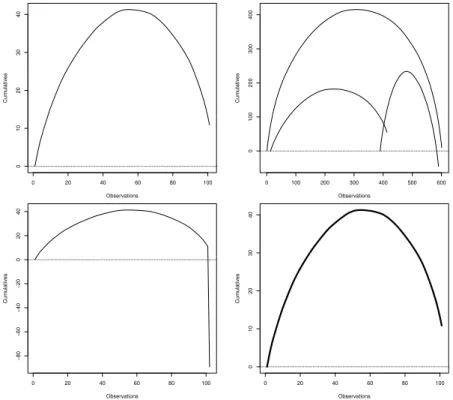
Figure 2: ccdplot()examples

(6)

The upper left graphics draws the Cumulative Characteristic Diagram of 100 random real numbers of standard normal distribution. This can be drawn with the following R function:

ccdplot(rnorm(100))

The upper right figure illustrates theComposite Cumulative Characteristic Dia- gram. This diagram contains characteristic diagram of two or more sets of numbers on the same scale, along with (the optional) the CCD of the union of the numbers.

The illustration contains numbers of normal distribution, with different size, different expected values and different variances. This can be created with help of R command

ccdplot(list(rnorm(400, 0.1, 1), rnorm(200, -0.1, 3))) The differences in width, height and the right end are spectacular.

The lower left diagram illustrates that this diagram is sensible on the outliers.

A mechanism is built in to remove the outliers automatically, either by providing an absolute threshold, or a percentage; the later one is applied on both ends. To reproduce a similar the diagram, use command

ccdplot(c(rnorm(100), -100))

Finally, the lower right diagram illustrates that the function integrates into the standard R diagram functions, the standard parameters can be passed. The line is thick, which can be achieved with the following command:

ccdplot(rnorm(100), lwd=5)

Detailed information about all the possible parameters and further examples can be obtained using the R help command:

?ccdplot qddplot()

This function creates Quantile Difference Diagrams. Figure 3 illustrates some examples.

The upper left diagram illustrates the comparison of two sets of random numbers of normal distribution, with different number of elements (100 vs. 200), different means (30 vs. 10) and different standard deviation. Despite the fact that the number of elements in the second subset is twice as much as in the first one, the illustration was possible. The diagram illustrates that the numbers in the first subset are higher than those in the second: the territory above the abscissa (i.e.

the x-coordinate) is higher than below it. On the other hand, it also illustrates that among the lowest elements the numbers in the second subset are higher than those in the first one. The diagram can be created using the following command:

(7)

−60−40−200204060

Quantile Differences

Quantile

Difference

0.1 0.2 0.3 0.4 0.5 0.6 0.7 0.8 0.9

−50050

Quantile

Difference

0 0.1 0.2 0.3 0.4 0.5 0.6 0.7 0.8 0.9 1

−10−50510

Different median, similar variance

−20...20 vs. −15...25 Quantile

Difference

0.1 0.2 0.3 0.4 0.5 0.6 0.7 0.8 0.9

−15−10−5051015

Similar median, different variance

−20...20 vs. −40...40 Quantile

Difference

0.1 0.2 0.3 0.4 0.5 0.6 0.7 0.8 0.9

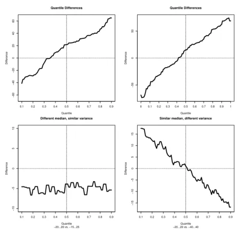
Figure 3: qddplot()examples

qddplot(rnorm(100, 30, 50), rnorm(200, 10, 10))

The upper right diagram illustrates that the diagram is biased at both ends.

This diagram is illustrated with numbers of the same distribution as above. By default, the diagram does not display the lower and the upper 5%. This can be fine-tuned using parameters. In this example the remove ratio is set to 0:

qddplot(rnorm(100, 30, 50), rnorm(200, 10, 10), remove.ratio=0.0) The primary usage of this diagram is intended to illustrate the comparison of two sets of numbers of the same distribution and similar variance, but different expected value. The first set contains 41 numbers, close to all the integers from -20 up to +20, and the second one similar numbers from -15 to +25. The difference is about 5, which is illustrated in the lower left diagram. The usage is intended to be converse: we have 2 sets of numbers, and the diagram reveals this property. The diagram was made using command

qddplot(seq(-20, 20) + rnorm(41), seq(-15, 25) + rnorm(41),

(8)

main = "Different median, similar variance", sub = "-20...20 vs. -15...25")

The second most important usage of the diagram is intended to be the variance comparison. In this example the first set of numbers contain similar elements as above, and the second one contains 81 elements, around the integers from -40 up to +40. The comparison statistic tests, which compare the mean or median of the numbers would not show relevant deflection, however, the diagram, as shown in the lower right, indicates that there is a difference in variance. The medians are more or less the same (the difference is around 0 at the median), but in the ends the line is far from 0. Therefore such an illustration would indicate it is worth to compare the variances. The diagrams was created using the following command:

qddplot(seq(-20, 20) + rnorm(41), seq(-40, 40) + rnorm(81), main = "Similar median, different variance",

sub = "-20...20 vs. -40...40")

Detailed information about all the possible parameters and further examples can be obtained using the R help command:

?qddplot projectdata

The package contains information about the following software systems: the well-known open source Ant, Struts 2 and Tomcat, and about an industrial software with nameGremon, which is a greenhouse monitoring system. In order to access the data first we need to issue the following command:

data(projectdata)

For each project a data frame is provided, containing information of every available commit. The rows of the data frame represent commits, and there are the following columns:

• A: number of added files

• U: number of updated files

• D: number of deleted files

• MaintainabilityDiff: maintainability difference caused by the commit The number of added, updated and deleted files are non negative integers, containing information about Java files (non Java files were removed). Commits not containing Java files were removed.

TheMaintainabilityDiffis the difference of maintainability values of 2 sub- sequent revisions. The maintainability of every revision was calculated with the

(9)

help of Columbus Quality Model [14]. These maintainability values were normal- ized and the difference was calculated as described in paper by Faragó et al. [15].

The final result is a real number.

This is an example excerpt of the data (information about the first 10 commits of project Ant):

> projectdata$Ant[1:10,]

A U D MaintainabilityDiff

1 44 0 0 0.00000

2 0 5 0 -14.55057

3 0 1 0 0.00000

4 0 2 1 -524.46238

5 1 1 1 -19.55645

6 0 3 0 -184.04878

7 0 3 0 -15.25897

8 0 1 0 -56.05360

9 0 2 0 16.39003

10 0 0 6 -71.82581

Detailed information can be obtained using the help page of the project data, using R command

?projectdata

4. Illustrating the statistic tests

In this section we provide some examples about the usage of the defined diagrams, illustrating various statistic tests.

For the illustration, first we generate sets of numbers. Both sets are of normal distribution, containing 101 elements each. The first subset’s (xin the example) mean is 1, and the standard deviation is also 1, and the second subset’s (yin the example) mean is -1, and the standard deviation is 3. For the data generation first we set the radom seed in order to be able to reproduce the results.

set.seed(1)

x <- rnorm(101, 1, 1) y <- rnorm(101, -1, 3)

In this example we act as we just received these sets of numbers, and we do not know anything about them. First we generate the Cumulative Characteristic Diagram and the Quantile Difference Diagram, and then begin with the analysis.

The diagram generation is performed with the following commands:

ccdplot(list(x, y)) qddplot(x, y)

The results are displayed in Figure 4.

(10)

0 50 100 150 200

−100−50050100150200

Observations

Cumulatives −10−50510

Quantile

Difference

0.1 0.2 0.3 0.4 0.5 0.6 0.7 0.8 0.9

Figure 4: Examples for statistic test demonstrations

4.1. Wilcoxon rank correlation tests and CCD

First let us check the Cumulative Characteristic Diagram (the left diagram of Fig- ure 4). Based on the difference of the altitude of the right end of the characteristic lines (the first one is far above 0, and the second one is far below 0) it indicates that it is likely that the elements in the first subset are significantly higher than those in the second. To check this, we perform a one tailed Wilcoxon rank correlation test (also known as Mann-Whitney U test). This test compares each elements of the first subset with each in the second one. The advantage of this test over the t-test (which performs the comparison on the averages) is that while t-test is very sensitive to outliers the Wilcoxon test does not.

This is the result of the Wilcoxon test:

> wilcox.test(x, y, alternative="greater")

Wilcoxon rank sum test with continuity correction data: x and y

W = 7843, p-value = 2.046e-11

alternative hypothesis: true location shift is greater than 0

The preliminary assumption based on the CCD turned to be correct: the p-value is very low. Conversely, having a good result of Wilcoxon test, we can illustrate it with CCD.

4.2. Wilcoxon rank correlation tests and QDD

The results so far indicates that the numbers in the first subset are greater than those in the second one. But can we tell more about them? To answer the question, consider the QDD (the right diagram of Figure 4).

The result of the Wilcoxon test on this diagram means the following: the signed territory between the line and the x coordinate is positive. However, on the right side

(11)

the line is below 0, meaning that just considering the highest values, those in the second data set are higher than in the first one. In concrete cases this worth further analysis.

Without QDD, this attribute could have been bypassed.

What does it mean in practice? Let the numbers denote the knowledge of students in mathematics in different countries. It can be higher in country A compared to country B in general, but the best students in country B might be better than in country A. On the Mathematics Olympics country B is likely to gain better results over country A. On the contrary: having a better results on the Olympics does not necessarily mean that the education is on the good way.

4.3. Variance tests and CCD

Considering the CCD again (the left diagram of Figure 4) there is another spectacular difference between the left and the right curve to note: their width are the same, but the vertical lengths of the lines are different: the right hand side is much longer than the left hand side. This indicates differences in variance. Let us perform the variance test!

> var.test(x, y, alternative="less") F test to compare two variances data: x and y

F = 0.095434, num df = 100, denom df = 100, p-value < 2.2e-16 alternative hypothesis: true ratio of variances is less than 1 95 percent confidence interval:

0.0000000 0.1328177 sample estimates:

ratio of variances 0.09543427

It turned out that the difference (indeed: the ratio) between the variance of the two subsets are really significant with extremely low p-value (meaning: it is very unlikely that this happened by chance).

It was not a big surprise for us as we generated the values to have different variances;

however if we act we do not know anything about the nature of the input data, this could be helpful. In our study such a diagram helped us to perform analysis in this direction, and we presented the result in article [16].

4.4. Variance tests and QDD

How does the difference in variance look like on the QDD?

If the line on the QDD is more or less horizontal, it indicates that there is no real difference in variance. On the other hand, if it has a slope, it is a sign of difference in variance. Considering the right diagram of Figure 4, we conclude that the line has a slope, indicating the probable significant difference of variances.

(12)

4.5. Contingency Chi-Squared tests and CCD

In the basic case of Chi-Squared tests we have a null hypothesis about the number of elements of some subsets, and real observations. For example, consider the genres of students in a university. The null hypothesis is that 50% are male and 50% are female.

In the fictive example of a Technical University there are 257 students, among them 243 boys and 14 girls. With the Chi-Squared test we can check if the difference is casual, or we should reject the null hypothesis, and state an alternative one, that in the technical universities there are more males then females.

In a more general case we have a matrix of any dimension. Every observation belongs to exactly one cell in the matrix. The null hypothesis is that the observations are dis- tributed evenly in the matrix. It does not exactly mean that the number of elements are the same in each cell, but it is calculated based on the row and the column sums.

In our example we consider a matrix of dimensions 2x2, containing the number of positive and negative elements in both subsets. The following listing contains how it was created, and then the values are displayed. Then the Chi-Squared test is performed, and the expected values, the global result of the test and the standard residuals on each cells are displayed. The meaning of the standard residual of a cell in nutshell is the following:

what was the difference between the expected and the actual value if it was a number of standard normal distribution. Based on this value, p-values can be calculated for each cell.

> sign <- matrix(c(length(x[x>0]), length(x[x<0]), length(y[y>0]), length(y[y<0])),

2, 2, dimnames=list(c("positive", "negative"), c("x", "y")))

> sign

x y positive 90 34 negative 11 67

> chisq.test.result <- chisq.test(sign)

> chisq.test.result$expected x y

positive 62 62 negative 39 39

> chisq.test.result

Pearson’s Chi-squared test with Yates’ continuity correction data: sign

X-squared = 63.177, df = 1, p-value = 1.889e-15

> chisq.test.result$stdres

x y

positive 8.092926 -8.092926 negative -8.092926 8.092926

>

The result of the Chi Squared test indicates that the number of positive and negative elements in sets xand yis significant. This is indeed not surprising for us, as we know the nature of numbers in the sets. But in general this is not known.

(13)

The connection between the result of the Chi-Squared test and CCD is the following:

if the shapes of the curves does not resemble to each other, with proper division it is likely that Chi-Squared test will show significant deflection from the null hypothesis (which in terms of CCD it means the shapes of the curves are similar).

In practice the Chi-Squared test is suggested to be executed specially in the following case: consider several observations (e.g. technical universities of different cities), and the curves on the CCD diagrams are different, but the CCD diagrams themselves are similar.

4.6. CCDs of the motivating examples

Figure 5 illustrates the CCD version of the motivating example (see 1 in Chapter 1.2).

The curves within diagrams are obviously different, and there are similarities between the diagrams. Therefore we found it more useful, compared to the boxplot version.

0 1000 3000 5000

02000060000

Ant − unbiased

(overall, delete, add, update+, update 1) Revisions

Accumulated maintainability change

0 200 600 1000

−5000500015000

Gremon − unbiased

0 500 1000 1500

01000020000

Struts2 − unbiased

0 200 600 1000

040008000

Tomcat − unbiased

Figure 5: Composite Cumulative Characteristic Diagrams about maintainability

(14)

5. Conclusions

In our earlier studies, we faced several problems in illustrating our achieved results visually.

However, visualization is very important as without it, using just text and tables, it is harder to explain and understand what we want to express. Furthermore, having just a bunch of numbers and p-values of test results it is hard to reveal patterns within the underlying data. For these reasons we introduced two new diagram types which are suitable for illustrating some of our results so far. Furthermore, we found it useful to forebode other significant connections not realized before.

In this paper we described these new diagram types, which we callCumulative Char- acteristic Diagram (CCD), andQuantile Difference Diagram (QDD). In general, both are suitable to visualize a numeric set of data. The Cumulative Characteristic Diagram itself is a curve that is based on the non-ascending order of the values, which are accumulated and plotted. The Quantile Difference Diagram illustrates the difference of two data sets on the same quantiles.

After an introduction and giving our motivations, we defined the diagram types and illustrated some possibilities for their application. We presented how they can be used for visualizing the results of Wilcoxon rank tests, variance tests and the CCD for contingency Chi-squared tests.

We implemented the diagram in the R statistic program in package vudc, and we also provided technical details about the usage of the implementedccdplotandqddplot R function, along with the data projectdataadded to this package. We described the parameters of these function in detail and provided examples of their use in practice.

Finally, we presented how these diagrams type helped us in illustrating the results of our research for revealing the effect of developer interactions on software maintainability.

With the help of these diagrams we were able to reveal some non-standard commits and outliers; finding and handling them properly helped us to achieve more meaningful results.

We demonstrated how these diagrams were suitable to illustrate the result of a concrete Chi-squared contingency test, then we provided some examples for visualizing the results of a Wilcoxon test and variance test.

Acknowledgments

The author would like to thank Rudolf Ferenc and Péter Hegedűs for providing advices to this article.

References

[1] J. M. Chambers, W. S. Cleveland, B. Kleiner, and P. A. Tukey, “Graphical methods for data analysis,” Wadsworth, Belmont, CA, 1983.

[2] P. Murrell,R Graphics. CRC Press, 2005.

[3] R. McGill, J. W. Tukey, and W. A. Larsen, “Variations of box plots,”The American Statistician, vol. 32, no. 1, pp. 12–16, 1978.

[4] Y. Benjamini, “Opening the box of a boxplot,” The American Statistician, vol. 42, no. 4, pp. 257–262, 1988.

(15)

[5] M. Frigge, D. C. Hoaglin, and B. Iglewicz, “Some implementations of the boxplot,”

The American Statistician, vol. 43, no. 1, pp. 50–54, 1989.

[6] K. Potter, H. Hagen, A. Kerren, and P. Dannenmann, “Methods for presenting statistical information: The box plot,” Visualization of Large and Unstructured Data Sets, s, vol. 4, pp. 97–106, 2006.

[7] J. L. Hintze and R. D. Nelson, “Violin plots: a box plot-density trace synergism,”

The American Statistician, vol. 52, no. 2, pp. 181–184, 1998.

[8] P. Kampstra, “Beanplot: A boxplot alternative for visual comparison of distribu- tions,” Journal of Statistical Software, Code Snippets, vol. 28, no. 1, pp. 1–9, 2008.

[9] K. M. Goldberg and B. Iglewicz, “Bivariate extensions of the boxplot,”Technometrics, vol. 34, no. 3, pp. 307–320, 1992.

[10] P. J. Rousseeuw, I. Ruts, and J. W. Tukey, “The bagplot: a bivariate boxplot,” The American Statistician, vol. 53, no. 4, pp. 382–387, 1999.

[11] K. Hornik, A. Zeileis, and D. Meyer, “The strucplot framework: Visualizing multi- way contingency tables with vcd,” Journal of Statistical Software, vol. 17, no. 3, pp.

1–48, 2006.

[12] D. Sarkar,Lattice: Multivariate Data Visualization with R. Springer, 2008.

[13] R Core Team, R: A Language and Environment for Statistical Computing, R Foundation for Statistical Computing, Vienna, Austria, 2015. [Online]. Available:

http://www.R-project.org/

[14] T. Bakota, P. Hegedűs, P. Körtvélyesi, R. Ferenc, and T. Gyimóthy, “A probabilistic software quality model,” in 2011 27th IEEE International Conference on Software Maintenance (ICSM). IEEE, 2011, pp. 243–252.

[15] C. Faragó, P. Hegedűs, and R. Ferenc, “The impact of version control operations on the quality change of the source code,” inComputational Science and Its Applications (ICCSA). Springer, 2014, pp. 353–369.

[16] C. Faragó, “Variance of source code quality change caused by version control operations,” Acta Cybernetica, vol. 22, pp. 35–56, 2015.