1 This is an unedited copy version. Please, cite the original paper as:
1
Lengyel A, Landucci F, Mucina L, Tsakalos JL, Botta‐Dukát Z. Joint optimization of cluster 2
number and abundance transformation for obtaining effective vegetation classifications. J 3
Veg Sci. 2018;29:336–347. https://doi.org/10.1111/jvs.12604 4
5 6 7 8
Joint optimization of cluster number and abundance transformation for obtaining 9
effective vegetation classifications 10
11
Attila Lengyel 1,2,* (lengyel.attila@okologia.mta.hu) 12
Flavia Landucci 3 (flavia.landucci@gmail.com) 13
Ladislav Mucina 4, 5 (laco.mucina@uwa.edu.au) 14
James Tsakalos 4 (james.tsakalos@research.uwa.edu.au) 15
Zoltán Botta-Dukát 1,6 (botta-dukat.zoltan@okologia.mta.hu) 16
17
1 MTA Centre for Ecological Research, Institute of Ecology and Botany, Alkotmány u. 2-4, 18
H-2163 Vácrátót, Hungary 19
2 Department of Vegetation Ecology, University of Wrocław, ul. Przybyszewskiego 63, 51- 20
148 Wrocław, Poland 21
2
3 Department of Botany and Zoology, Masaryk University, Kotlářská 2, CZ-611 37 Brno, 22
Czech Republic 23
4 School of Biological Sciences, The University of Western Australia, 35 Stirling Hwy, 24
Crawley WA 6009, Perth, Australia 25
5 Department of Geography & Environmental Studies, Stellenbosch University, Private Bag 26
X1, Matieland 7602, Stellenbosch, South Africa 27
6MTA Centre for Ecological Research, GINOP Sustainable Ecosystems Group, Klebelsberg 28
Kuno u. 3, H-8237 Tihany, Hungary 29
30
*Corresponding author 31
32
Abstract 33
Question: Is it possible to determine which combination of cluster number and taxon 34
abundance transformation would produce the most effective classification of vegetation data?
35
What is the effect of changing cluster number and taxon abundance weighting (applied 36
simultaneously) on the stability and biological interpretation of vegetation classifications?
37
Locality: Europe, Western Australia, simulated data 38
Methods: Real data sets representing Hungarian submontane grasslands, European wetlands, 39
and Western Australian kwongan vegetation, as well as simulated data sets were used. The 40
data sets were classified using the partitioning around medoids method. We generated 41
classification solutions by gradually changing the transformation exponent applied to the 42
species projected covers and the number of clusters. The effectiveness of each classification 43
was assessed by a stability index. This index is based on bootstrap resampling of the original 44
data set with subsequent elimination of duplicates. The vegetation types delimited by the most 45
stable classification were compared with other classifications obtained at local maxima of the 46
stability values. The effect of changing the transformation power exponent on the number of 47
clusters, indexed according to their stability, was evaluated.
48
3 Results: The optimal number of clusters varied with the power exponent in all cases, both 49
with real and simulated data sets. With the real data sets, optimal cluster numbers obtained 50
with different data transformations recovered interpretable biological patterns. Using the 51
simulated data, the optima of stability values identified the simulated number of clusters 52
correctly in most cases.
53
Conclusions: With changing the settings of data transformation and the number of clusters, 54
classifications of different stability can be produced. Highly stable classifications can be 55
obtained from different settings for cluster number and data transformation. Despite similarly 56
high stability, such classifications may reveal contrasting biological patterns, thus suggesting 57
different interpretations. We suggest testing a wide range of available combinations to find 58
the parameters resulting in the most effective classifications.
59 60
Keywords 61
Clustering; Cluster validation; Community similarity; Cover scale; Data type; Multivariate 62
data analysis; Numerical classification; Stability of classification 63
64
Abreviations 65
MSL = mean standardized lambda; PAM = partitioning around medoids; PCoA = principal 66
coordinate analysis 67
68
Nomenclature 69
The names of high-rank European syntaxa follow Mucina et al. (2016).
70 71
Introduction 72
4 Numerical methods are applied in vegetation classification studies to reduce the
73
dimensionality of the data in seeking patterns, to increase objectivity in the analyses, and thus 74
to enhance the reproducibility of results. Still, classification protocols often rely on subjective 75
decisions that can significantly influence the results (De Cáceres et al. 2015). Subjective 76
choices can hardly be avoided, yet they should be well-informed and logical to make the 77
analytical procedures reliable and repeatable. In numerical classifications, according to 78
Lengyel & Podani (2015), the choice of the number of clusters and the weight attributed to 79
abundant species relative to scarce species (hence the data transformation), are among the 80
most influential decisions that have to be considered carefully. If the aim of the classification 81
is to delimit a pre-set number of vegetation types within the data set, then the choice of the 82
resulting clusters should be guided by practical considerations. In certain cases there is 83
reasonable external information available for selecting a transformation function as well. For 84
instance, if the abundance estimations are deemed inaccurate, only presence/absence data 85
should be used. Equally, if the purpose of the study is to analyse vegetation types 86
characterised by dominant species, it is more logical to apply a transformation giving high 87
emphasis to differences in species abundance. However, if the aim of the classification is to 88
explore variation by separating and differentiating vegetation types, classifications using a 89
suite of contrasting parameters should be produced. These should be evaluated a posteriori in 90
order to identify the optimal parameter values yielding in the ‘best’ (according to the set 91
criteria) classification.
92
The optimal number of clusters can be sought for by calculating cluster effectiveness (or 93
validity) index for classifications with increasing number of clusters. Thus, the optimal 94
number of clusters is the one where the effectiveness index reaches maximum or minimum, 95
depending on scaling. This procedure is widely known and regularly applied in classification 96
studies (e.g. Botta-Dukát et al. 2005; Tichý et al. 2010, 2011). However, we are aware of only 97
a few examples when authors evaluated different data transformations for finding the optimal 98
weighting of abundances that would reveal biological patters most effectively or would lead 99
to the most stable results. Jensen (1978) evaluated the effect of several data transformations 100
on classifications and ordinations of a lake vegetation data, and concluded that ‘extreme 101
transformations’ (i.e. those giving high weight either to high abundance values or, in reverse, 102
to presence/absence data) can yield significantly different results. This finding was 103
corroborated by Campbell (1978) and van der Maarel (1979). Wilson (2012) compared the 104
stability of ordination analyses performed on various vegetation samples using different 105
5 transformations of abundance and concluded that the ‘optimal’ transformations depend on 106
context, such as geographical extent, environmental heterogeneity, disturbance status of the 107
study area, and quality of abundance estimations. Although, any ‘optimal’ parameterization 108
supposed to produce a robust classification is specific for the actual data set, the low interest 109
of researchers in finding them, or at least in assessing the performance of methods they apply, 110
is surprising, given that vastly different results can be achieved by application of different 111
abundance scales in multivariate analyses – a fact well known for long time (Austin & Greig- 112
Smith 1968; Noy-Meir et al. 1975; van der Maarel 1979).
113
In this paper, we introduce a procedure for choosing the combination of two factors, namely 114
(1) the number of clusters and (2) varying scale of transformation power, assisting in 115
identification of the most effective classification outcome. Like other approaches aimed at 116
determination of the optimal number of clusters (e.g. Aho et al. 2008), a general guideline for 117
finding the optimal transformation would be to find the function that leads to the most stable 118
of several possible classifications produced by differently parameterized transformation 119
functions. We show that changing one of these two factors has an impact on the optimal 120
values of the other, which influences the biological interpretation of the classification result, 121
and therefore we promote their joint optimization. We test this approach using real and 122
simulated data sets.
123 124
Materials and methods 125
Grasslands data set 126
The Grasslands data set consists of phytosociological plots collected in the colline and 127
montane belts of northern Hungary. This data set represents different types of mesic, 128
unproductive to moderately productive, grazed, mown, and recently abandoned grasslands on 129
neutral to acidic soils. Several types can be recognized by their dominant species, e.g.
130
Agrostis capillaris, Arrhenatherum elatius, Danthonia decumbens, Festuca rubra and Nardus 131
stricta. However, these types are not floristically distinctly separated, and stands with 132
different dominant species can be similar in the overall species composition.
133
Wetlands data set 134
6 The Wetlands data set was extracted from the WetVegEurope database (Landucci et al. 2015).
135
It contains plots from Austria, Czech Republic, Germany, Hungary, Poland, Slovakia, and the 136
Netherlands. In these plots the diagnostic species of the class Phragmito-Magnocaricetea 137
(according to Mucina et al. 2016) should have dominance of at least 25% of the total cover.
138
Only plots having at least five species and plot sizes between 15 and 50 m2 were included.
139
The data set was subject to geographical stratification and to heterogeneity-constrained 140
random resampling (Lengyel et al. 2011) as modified by Wiser & De Cáceres (2013) in order 141
to avoid pseudo-replications and maximally diversify the dataset. In this data set, several 142
types can be distinguished on basis of dominant species, however many of these communities 143
share similar species pool. Therefore, classifications are expected to vary with changing 144
power of the data transformation.
145
Kwongan data set 146
The Kwongan data set is composed of 375 plots of natural shrubland (heath-like) vegetation 147
of the Geraldton Sandplains (surrounds of the Eneabba township), Western Australia. This 148
unique, endemic-rich vegetation is supported by sandy soils extremely depleted in phosphorus 149
(and also nitrogen) – a product of prolonged tectonic quiescence of the Western Australian 150
landscapes spanning hundreds of millions of years, resulting in lack of soil rejuvenation and 151
progressive nutrient leaching, combined with relatively stable and predictable climatic 152
seasonality, and predictable natural fire disturbance (Lambers 2014). This data set exemplifies 153
an unusual, yet real situation: both alpha and beta diversity are high, resulting in high regional 154
species pool (gamma diversity). Species dominance (in terms of biomass and projected cover) 155
in this vegetation is supressed. We expect that the classification outcomes would be quite 156
resistant to changes of the magnitude of the data transformation.
157
Characteristics of the three data sets are summarized in Table 1. A more in-depth analysis of 158
the Grasslands data set is presented, while we focused on the relationship between the 159
examined methodological decisions and classification stability in the Wetlands and the 160
Kwongan data sets.
161
Simulated data 162
Simulated data matrices consist of N plots (in the rows) and S species (in the columns). Plots 163
belong to K clusters of equal size, thus the number of plots is N/K = n in each cluster, and n is 164
7 a pre-defined integer. Ten species occur in each cluster and each species occurs in two
165
clusters, thus S = 10 × K/2. Each species has constant abundance across plots within a cluster, 166
while the abundances may differ among clusters. The abundances of species within one of the 167
two clusters where they occur, are drawn from a Poisson-lognormal distribution (Bulmer 168
1974) where the mean and the standard deviation (SD) of the lognormal distribution are (2; 1) 169
on log scale. For the other cluster, the order of abundances is reversed, thus if a species was 170
the most abundant in one of the clusters where it occurs, then this species will be the least 171
abundant in the other one (considering only species occurring in this cluster). These matrices, 172
therefore, consist of plots of K clusters according to raw abundances of species, but K/2 173
clusters according to presence/absence data because pairs of clusters share the same species 174
occurring with different abundances. We expect the optimal number of clusters to be K/2 with 175
low exponents, while with high exponents optimal solution should comprise K clusters.
176
Notably, abundance-based clusters are nested within clusters based on presence/absence data.
177
Within each cluster, plots are identical, thus the clustered structure is initially perfect. An 178
exemplary matrix is shown in Appendix S1. Then, noise was added to this initial matrix 179
following the method of Gotelli (2000) used for ‘noise test’, but applied to abundances instead 180
of presence/absence data. This procedure applies a swapping algorithm to introduce noise. In 181
a single swap, the rows and columns of the original matrix are permuted, and a 2 × 2 182
submatrix with positive values in the diagonal is chosen randomly. Then the two diagonal 183
cells are decreased by 1, while abundances in the two off-diagonal cells are increased by 1 184
individual, thus the sum and the marginal totals of the submatrix do not change. Finally, the 185
original order of rows and columns is restored. A single swap would affect a sparse matrix 186
more than one with high fill. Also, large matrices are more ‘resistant’ to the same number of 187
swaps than small ones. Therefore, noise is added to the matrices in discrete levels, one level 188
consisting of as many swaps as the number of non-zero elements in the matrix. Our 189
preliminary analyses suggested that in this way a comparable amount of stochasticity can be 190
added to matrices of different size and fill.
191
Five simulation series were performed, each of them with five different set-ups. In these 192
series, one or two parameters were changed systematically in order to generate simulated 193
matrices that would differ in: i) noise level; ii) size of clusters with number of clusters fixed;
194
iii) number of clusters with cluster sizes fixed; iv) number and size of clusters with total 195
number of plots fixed; v) dominance of species. The dominance was changed by modifying 196
the SD of the lognormal distribution used as input for the Poisson process of species 197
8 abundances. When SD is high, there is one or a few highly dominant species within a plot and 198
many very scarce species, while with lower SD species abundances should be balanced.
199
Classification method 200
For classifying the data sets, we used the partitioning around medoids method (PAM;
201
Kaufman & Rousseeuw 1990) using Marczewski-Steinhaus index as the measure of 202
dissimilarity (Appendix S2). For the Grasslands and Kwongan data set covers of species were 203
directly estimated on percentage scale in the field, while for the Wetlands data set, 204
abundances were mostly recorded on Braun-Blanquet or finer ordinal scales. These ordinal 205
categories were replaced by their midpoint percentages. Cover percentages were power 206
transformed using the function x´ = xa, where x is the original cover value on percentage 207
scale, a is the power exponent, and x´ is the transformed cover value. The power exponent 208
was gradually changed from 0 to 1, with 21 steps by 0.05 in between in case of real data, and 209
with steps of 0.1 in case of simulations where simpler patterns were expected. Low values of 210
the exponent reduce the effect of differences between species abundances, thus giving more 211
weight to rare species, while values near 1 give more weight to abundant species. The lowest 212
number of clusters examined was 2. The highest number of examined clusters was 10 for the 213
Grasslands data, 40 for the Wetlands and for the Kwongan data, and it varied in simulations 214
according to the pre-defined number of clusters and sample size. The maximal number of 215
clusters was arbitrarily determined to balance between computation time and the number of 216
practically distinguishable vegetation types.
217
Evaluation of classifications 218
Several approaches for evaluating classifications exist, and each of them involves numerous 219
indices (e.g. Milligan & Cooper 1985; Vendramin et al. 2010). These approaches include 220
correlating the original distances between objects and their representations in the 221
classification (e.g. Rohlf 1974), measuring compactness, connectedness, and separation of 222
clusters (e.g. Popma et al. 1983), assessing the robustness of the results to changes in 223
methodological decisions and choice of variables (e.g. Chiang & Mirkin 2010), repetitiveness 224
(e.g. McIntyre & Blashfield 1980), stability (e.g. Hennig 2007), interpretability (e.g. Tichý et 225
al. 2010), and predictive power (e.g. Lyons et al. 2016) of the classification, and degree of 226
divergence from a random classification (e.g. Hunter & McCoy 2004).
227
9 A family of classification effectiveness (or validity) measures called geometric indices (Aho 228
et al. 2008) rely on dissimilarities between plots which involve a decision on the weighting of 229
species abundances. For example, if an effectiveness index uses resemblances calculated by 230
the Jaccard index (Podani 2000) using presence/absence data, then the classifications 231
produced on the basis of binary occurrences of species are likely to seem to be ‘better’ than 232
classifications based on cover percentages. However, not only geometric indices need 233
decisions on data transformation. The non-geometric OptimClass indices (Tichý et al. 2010), 234
which use the number of characteristic species of clusters as the measure of effectiveness, can 235
be calculated from both presence/absence and cover percentage data. As the form of cover 236
transformation is known to strongly affect the fidelity values of species (Willner et al. 2009), 237
it is expected that classifications based on presence/absence data would have more character 238
species, if only binary occurrences are considered for fidelity calculations, while 239
classifications using cover data would seem less effective.
240
For an unbiased comparison of effectiveness among classifications based on different data 241
transformations and cluster numbers, it is necessary to compare all classifications to a 242
standardized reference. The stability index, introduced by Tichý et al. (2011), meets this 243
criterion. It compares the classification of plots in the original data set with classifications of 244
its subsets selected by bootstrap resampling with subsequent elimination of duplicates (Tichý 245
et al. 2011). The similarity between the cluster assignments of resampled plots in the original 246
classification and in the classification of the subset is calculated using the mean standardized 247
lambda (hereafter called MSL), the standardized version of Goodman & Kruskal’s lambda 248
index (Goodman & Kruskal 1954; Appendix S2). In our analysis, we used 50 without- 249
replacement bootstrap samples for each classification produced by different cluster numbers 250
and data transformations. MSL was plotted on a so-called heat map, in which the colour of 251
the respective segment of the space defined by two explanatory variables (i.e. the power 252
exponent and cluster number) refers to the magnitude of the dependent variable (i.e. MSL).
253
The marginal distribution of the heat map can also be examined for determining those 254
parameter values which are likely to provide the most effective classification ourcomes, or the 255
lowest or highest variation in classification stability. If one of the parameters, e.g. the 256
exponent, is fixed to an actual value, the mean of the MSL values obtained with changing the 257
other parameter, that is the number of clusters, gives how stable the classifications obtained 258
with the actual exponent are on average. By using the SD instead of the mean, the variation of 259
10 stability can be expressed, too. Therefore, the SD is a measure of how important the decision 260
is about one of the two parameters if the other one is fixed to an actual value. The use of 261
marginal distributions is showed only for the Grasslands data set.
262
The most stable classification of a real data set (i.e. the classification with settings resulting in 263
the absolute maximum of MSL and the darkest segment on the heat map) was evaluated by 264
creating a synoptic table containing frequency, average percentage cover, and fidelity of 265
species. The fidelity of species to clusters was calculated using the phi coefficient on 0 to 100 266
scale (Chytrý et al. 2002). Species with phi value over 20 were considered ‘characteristic’, 267
and only species with Fisher exact test p<0.001 were considered. Classifications at the 268
optimal cluster level obtained by different exponents, with special attention to the commonly 269
used values (a = 0, 0.5 or 1) and local peaks in stability, were compared on basis of the group 270
memberships of plots using cross-tabulations, as well as by contrasting their biological 271
interpretation with the help of characteristic species.
272
Data analyses were performed in the R software environment (version 3.1.2, www.r- 273
project.org) using the vegan (Oksanen et al., http://cran.r-project.org/package=vegan), cluster 274
(Maechler et al., http://cran.r-project.org/package=cluster), rapport (Blagotić & Daróczi, 275
http://cran.r-project.org/package=rapport), and fields (Nychka et al., http://cran.r- 276
project.org/package=fields) packages. R scripts for data simulation, swapping and the 277
optimization procedure are available in the Appendix S3. We used Juice (Tichý 2002) for data 278
management and construction of synoptic tables.
279 280
Results 281
Grasslands data set 282
The heat map (Fig. 1) showed that the MSL values varied considerably across cluster number 283
and power exponent. With presence/absence data (a = 0), stability was the highest at the five- 284
cluster solution. From a = 0.05 to a = 0.25, the three-cluster level was the most stable, 285
including a = 0.15 where the second highest stability value was obtained (MSL = 0.804).
286
Between a = 0.3 and a = 0.4, the stability peaked at two clusters, then from a = 0.45 the four- 287
cluster solution was optimal until a = 0.90, while for the higher exponent values again three 288
11 clusters were shown to be the best. The absolute maximum value was found with a = 0.55 and 289
the four-cluster solution, where the stability of the classification was MSL = 0.824. Exponents 290
between a = 0.25 and 0.50 resulted in the highest stability values on average, and the SD of 291
stability was also the lowest in this interval (Fig. 2). Nevertheless, a second local optimum 292
was found at a = 0.8, although the SD was much bigger here. Across the cluster levels, the 293
three- and four-cluster solutions were the most stable on average, while stability values did 294
not vary much, except for 2 clusters where SD was the highest.
295
We used the most stable classification (i.e. four clusters and exponent 0.55; hereafter called 296
‘Partition A’) as the baseline for the interpretation of all clusters and classifications (Appendix 297
S4). This classification was identical with what was obtained by a = 0.50, that is, square-root 298
transformation. Clusters A1, A2, A3, and A4 are the elements of the Partition A. Cluster A1 299
represents grasslands of the alliance Violion caninae, but some species of the mesic meadows 300
of the order Arrhenatheretalia are also frequent. Cluster A2 contains plots of the 301
Arrhenatherion. This type was recently described as the Diantho-Arrhenatheretum 302
association by Lengyel et al. (2016); it represents nutrient-poor, acidic grasslands overgrown 303
by taller grasses (e.g. Helictotrichon pubescens, Arrhenatherum elatius) after abandonment or 304
changing management to mowing. Cluster A3 comprises unproductive meadows and pastures 305
dominated by Agrostis capillatis, Festuca rubra, and Galium verum. These stands are similar 306
in species composition to the Anthoxantho-Agrostietum, known also from Slovakia and the 307
Czech Republic. Cluster A3 is also intermediate between Arrhenatheretalia and Violion 308
caninae. Cluster A4 contains grasslands dominated by Nardus stricta, in which species of 309
waterlogged soils are also present. This type is traditionally also called ‘Hygro-Nardetum’
310
(e.g. Borhidi et al. 2012).
311
In the presence/absence case (a = 0), five clusters were differentiated. Hereafter, this 312
classification is called ‘Partition B’. Cluster B1 included many plots of Cluster A1 and A3, 313
thus representing mesic meadows with some species of the Violion caninae, and matching the 314
species composition of Anthoxantho-Agrostietum. Cluster B2 and B3 contained mostly plots 315
previously classified to A2, thus differentiating between two subtypes of Diantho- 316
Arrhenatheretum: one with more hygrophilous, and one with more forest-steppe species, 317
respectively. Cluster B4 represents the ‘Hygro-Nardetum’ type, thus is similar to Cluster A4.
318
Cluster B5 contains only two plots similar to the Anthoxantho-Agrostietum.
319
12 With a = 0.15 and three clusters a local peak was detected, to be referred to as Partition C.
320
Cluster C1 contains many plots representing the types mediating between the 321
Arrhenatheretalia and Violion caninae, formerly classified to Clusters A1 and A3. Cluster C2 322
represents the Diantho-Arrhenatheretum, and it is very similar to Cluster A2. Cluster C3 323
represents the ‘Hygro-Nardetum’ and matches with Cluster A4.
324
With a = 1 (= no data transformation), three clusters provided the most stable resolution. This 325
classification was called Partition D. Cluster D1 represents grasslands on nutrient-poor soils, 326
including the ‘Hygro-Nardetum’ and other types related to the Violion caninae and containing 327
Nardus stricta. It contains plots of Cluster A1 and A4. Cluster D2 represents mesic hay 328
meadows with Arrhenatherum elatius, and it shares many plots with Cluster A2. Cluster D3 329
represents unproductive meadows and pastures with the dominance of Agrostis capillaris, 330
Briza media and Festuca rubra. Most of its plots were assigned to Cluster A3 and C2.
331
Therefore, the Partitions C and D similarly separated the Diantho-Arrhenatheretum from 332
other types, but differed in how they delimited two other clusters in the rest of the data set.
333
The cross-tabulation of Partition A against Partitions B, C and D, as well as Partition C 334
against Partition D are shown in Appendix S5.
335
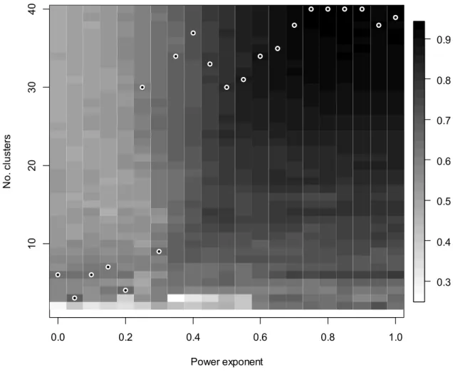
Wetlands data set 336
The optimal number of clusters ranged between 3 and 7 when the exponent ranged between 0 337
and 0.20 (Fig. 3). With higher exponents, the optimal cluster levels increased, too; from a = 338
0.35 the most stable classifications were found at levels of more than 30 clusters. In the binary 339
case (a = 0), the optimal cluster level was 6, with the square-root transformation (a = 0.5) it 340
was 30, with no transformation (a = 1) it was 39. The most stable classification was the one 341
with a = 0.80 and 40 clusters where MSL was 0.933. At this level clusters were distinguished 342
according to dominant species that were both constant and character species in many cases.
343
Using other high exponents (e.g. a = 0.50 or a = 1) resulted in very similar classifications, 344
thus only the comparison of solutions with a = 0 (hereafter called ‘Partition W’) and a = 0.80 345
(‘Partition Z’) are presented using synoptic tables (Appendix S6 and S7, respectively). Since 346
many phytosociological associations and alliances of wetland vegetation are defined by 347
dominant species, classifications with high exponents (Partition Z) showed a good 348
correspondence with low-rank syntaxa. With low exponents, the most stable classifications 349
revealed markedly different patterns that were difficult to interpret, yet these local optima 350
13 possessed much lower stability. With a = 0 (Partition W) differences in species pools offered 351
some, although not fully satisfactory explanation for the distinction of clusters. Cluster W1 352
contained many plots of tall-sedge vegetation with short submerged periods and eutrophic 353
soils (supporting mostly Magnocaricion gracilis vegetation). Cluster W2 included mostly 354
plots of tall-sedge vegetation on sites with poorer nutrient supply (mostly Magnocaricion 355
gracilis and Magnocaricion elatae). Cluster W3 is characterised, to a large part, by reed 356
vegetation belonging to the Phragmition and Phalaridion. Clusters W4 and W5 contained 357
many plots sampled in wetlands characterised by fluctuating shallow waters (mostly 358
Eleocharito-Sagittario, Phramition, Glycerio-Sparganion), however no clear ecological 359
difference could be recognized between them. Cluster W6 included plots from nutrient-poor 360
mire vegetation often classified as the Scheuchzerio-Caricetea. Obviously, Partition W 361
showed very low congruence with the syntaxonomical system and Parition Z (Appendix S8).
362
Classifications with a = 0 and a = 0.80 do not differ only in the resolution. As it is shown in 363
Appendix S8, clusters of the latter are not nested within the former, instead, it is very common 364
that plots classified to the same cluster at a = 0.80 are assigned to different clusters at a = 0.
365
Kwongan data set 366
MSL values varied much at low levels of cluster numbers (up to 6 clusters) and showed much 367
less (and also less predictable) variability at cluster levels above 6 (Fig. 4). The highest MSL 368
values occurred at the cluster levels 2 and 4. The highest classification stability was detected 369
at the 4-cluster level (for exponents spanning 0.0 and 0.75) or the 2-cluster level (for 370
exponents spanning 0.8 and 1.0). The most stable classification was obtained with a = 0.95, 371
cluster number = 2, with stability MSL = 0.843.
372
At a = 0, four clusters were distinguished (Partition K; Appendix S9). Cluster K1 represented 373
a community with typical species Hakea candolleana and Allocasuarina humilis found on 374
free-draining soils. Cluster K2 was identified as Xylomelum angustifolium-Banskia menziesii 375
community thriving on sandy soils on dune swells. Cluster K3 included plots from 376
Ecdeiocolea monostachya-Scholtzia laxiflora community occurring on sandy soils with 377
slightly elevated clay content in inter-dune depressions, while Cluster K4 represented Banksia 378
shuttleworthiana-Cristonia biloba confined to regolith composed of depositional lateritic 379
scree and sand. Therefore, these clusters represented an edaphic gradient spanning Cluster K2 380
(deep sandy soils from the sand dune swells) and Cluster K3 (depressions showing elevated 381
14 clay content), with Clusters K1 and K4 occupying intermediate position along the gradient. At 382
a = 0.95, the 2-cluster solution was the most stable one (Partition L; Appendix S10). The 383
cross-tabulation tables (Appendix S11) showed that all plots of the Cluster K3 were assigned 384
to the Cluster L1 - the only cluster whose plots were assigned to the same cluster in Partitions 385
K and L. The Cluster K1 was concentrated in Cluster L1, while most plots of the Clusters K2 386
and K4 belonged to L2. Partitions K and L similarly recovered the gradient between 387
vegetation types supported by soils having elevated clay content (represented by Clusters K1 388
& K3, as well as L1) and sandy soils (as Clusters K2 & K4, and L2) on the basis of 389
characteristic species of the clusters. The relative position of the clusters in a PCoA ordination 390
also supports the notion that the main compositional patterns are similarly revealed by 391
different abundance weighting (Appendix S12).
392
Simulations 393
At the noise level 1, where abundances were strongly down-weighted (a = 0 or a = 0.1), the 394
stability was highest at the pre-defined number of four species-pool based clusters (Fig. 5).
395
From a = 0.2 to a = 0.7, two peaks were found, namely at the 4- and 8-cluster levels, the latter 396
being of higher stability, and with one intermediate peak at a = 0.3 and seven clusters. Where 397
abundance differences were not or only slightly reduced (a > 0.7), only the 8-cluster peak was 398
obvious. From the noise level 2 and higher, the stability peaked at the 8-cluster level. As more 399
levels of noise were added, classifications with low exponent were becoming less and less 400
stable.
401
Two optimal cluster levels were found where the number of plots in each cluster was 5 (Fig.
402
6). From a = 0 to a = 0.4, the 4-cluster peak (corresponding the species-pool-based number of 403
clusters) was higher, but from a = 0.5 to a = 1 the 8-cluster solution (i.e. the abundance based 404
optimum) was the most stable one. The pattern of stability was similar, although, less distinct, 405
with clusters of 10 and 25 plots. However, with 50 plots per cluster, the locations of the 406
optima were more irregular, with several peaks between four and eight clusters. With 100 407
plots per cluster, the optima were detected at four clusters for most of the exponent values, 408
except for a = 0.3 and a = 0.4.
409
When the number of clusters increased from four with constant cluster sizes, the typical 410
pattern of lower optima at low exponents and higher optima at high exponents were found in 411
most cases, yet with some exceptions (Fig. 7). Where the species-pool based cluster number 412
15 was two and the abundance-based cluster number was four, three clusters were the most stable 413
with low exponent and four with high exponent. With higher number of true clusters, the most 414
stable classification identified the pre-defined cluster numbers correctly: 8, 12, 16, and 24 415
clusters with higher exponents, and 4, 6, 8, and 12 clusters with lowers exponents, 416
respectively. The point of inflection, when the observed optima shifted from the species-pool- 417
based level to the abundance-based level, was variable. Yet a broad interval with at least two 418
local peaks of stability was detectable in all heat maps at intermediate exponent values.
419
Cluster numbers between the species-pool-based and the abundance-based optima also came 420
out as optimal in some cases, especially with exponents near the inflection value.
421
A very similar pattern was found when the number of clusters and cluster sizes were changed 422
with constant sample size (Appendix S13). The species-pool-based and the abundance-based 423
cluster numbers were recovered correctly as local or global peaks. Between them, 424
intermediate levels also gained high stability values, but they were identified as optimal only 425
in a few cases.
426
With SD = 0.1 the optimal cluster level was four clusters irrespective of the exponent value 427
(Appendix S13). Using a > 0.5 classifications of 7 and 8 groups showed local peaks. With 428
increasing SD, the stability of classifications with eight clusters and high exponent also 429
increased. With SD = 4, the 8-cluster solutions appeared the most stable, except for when a = 430
0, that is, in the binary case.
431
Discussion 432
Evaluation of the real data 433
The choice of data transformation and cluster number influences the delimitation of 434
vegetation types, as concluded in several other studies (e.g. Jensen 1978; Lengyel & Podani 435
2015). Certain types (e.g. Diantho-Arrhenatheretum in the Grasslands data set) are relatively 436
robust to changes in the examined parameters, while others (e.g. transitional types between 437
Arrhenatheretalia and Violion caninae) are more sensitive. When it comes to making an 438
unambiguous distinction between vegetation types for practical (such as management) 439
purposes or syntaxonomical revision, it is crucial to consider that different weighting of 440
abundant species may have implications for the delimitation of vegetation units, and thus for 441
the future applicability of the classification.
442
16 The Wetlands data set showed that the optimal cluster level can markedly differ if different 443
data transformations are used. While presence/absence data yielded six stable clusters that 444
represented types with more or less different species pools, accounting for differences in 445
abundances raised the optimal levels over 30, where each cluster is separated according to the 446
dominant species. The fact that the high number of stable clusters obtained using high 447
exponent were not nested within the few stable clusters based on presence/absence data, is a 448
clear indication that different data transformations can reveal different types of biological 449
patterns. With low exponents, classifications were best explained by patterns generated by 450
habitat-specific species-pools, while with high exponents, community types differing in fine- 451
scale environmental variation, temporal variability and site history were revealed. It is of 452
interest, that in our study, 40 clusters was the finest classification level examined due to a 453
compromise between practical and scientific reasons, but in reality the optimal number of 454
clusters in the Wetlands data set could have been even higher.
455
The Kwongan data provided a special insight into the interaction of data transformation and 456
cluster number. Changing the exponent changed the optimal number of clusters as well, and 457
the resulting stable classifications were moderately congruent. However, even these, 458
seemingly less similar classifications revealed the most important ecological pattern on the 459
basis of faithful species ― the soil gradient, although fine patterns of transitional subtypes 460
between the extremes were not detected equally well. The Kwongan data set, due to its high 461
beta diversity and balanced within-plot abundance distribution, was less sensitive to changes 462
in data transformation and cluster number in terms of biological interpretation, even though 463
the assignment of plots showed some variation.
464
Lessons from the simulations 465
In the simulations, we generated data structure with contrasting patterns with respect to 466
occurrence information. If abundance information were emphasized, the true number of 467
clusters (vegetation types) was twice as high as in cases where only presence/absence data 468
were considered, hence we differentiated a ‘species-pool-based’ and an ‘abundance-based’
469
number of clusters. In reality, however, also an opposite can be observed, where a few species 470
can be dominant in habitats with different species pools. In such a case the number of 471
abundance-based clusters could be lower than those based on species-pools, as it was seen 472
with the Kwongan data set.
473
17 We expected that weak data transformations (the exponent being close to 1) which preserve 474
the differences in original abundance patterns, would yield a higher cluster number, while 475
strong transformations (the exponent approaching 0) which significantly reduce abundance 476
differences would find the half of this number of clusters optimal. Our results confirmed this 477
expectation.
478
We introduced stochasticity to artificial data using a similar method as that by Gotelli (2000) 479
called ‘noise test’. This type of noise made classifications with stronger transformations less 480
stable than those involving weak transformations. This result can be understood by recalling 481
how we generated species abundances and noise. The species abundances had been drawn 482
from a Poisson-lognormal distribution, which resulted in many scarce and few abundant 483
species. Considering that the artificial matrices are designed in a way that their matrix fill is 484
low, swapping individuals can moderately reduce the abundance of species in a plot, or it can 485
slightly increase less abundant species, or make absent species present with low abundance.
486
However, it is unlikely to make an abundant species absent in a plot, or to make an absent 487
species very abundant. As a result, the applied noise affected binary information more than 488
the proportions of abundances which determine classifications involving weak data 489
transformations. We believe that this type of noise simulates a common form of stochasticity 490
in nature that is caused by random death of individuals followed by random colonization.
491
The simulations have revealed several tendencies in classification stability as related to cluster 492
number, data transformation, and sample properties. With increasing size of clusters, the 493
number of abundance-based clusters was underestimated, while the number of clusters based 494
on species pools was detected correctly. Despite this observation with both fixed and 495
changing total sample size, we cannot offer a clear explanation for this finding.
496
Based on the tests with modified pre-defined number of clusters with fixed cluster sizes, the 497
stability as optimality criterion seems to track the changes correctly in most cases. However, 498
when the number of clusters based on presence/absence data was two, the most stable 499
classifications were obtained at the three-cluster level with strong transformation. (With weak 500
transformations, the abundance-based number of clusters was correctly found at the level of 501
four clusters.) Moreover, in a few cases, optima were indicated between the species-pool- 502
based and the abundance-based levels. When the total sample size was fixed, but number and 503
size of clusters changed, stability performed similarly well. Some inconsistency was found at 504
four abundance-based clusters, where the most stable level was found at two clusters for all 505
18 but one value of the exponent. Surprisingly, the exception was the binary case (a = 0) where 506
all classifications were generally less stable and the optimum was at the pre-defined number 507
of clusters based on abundance, i.e. four clusters. This contradicts our expectation and we 508
have no clear explanation for this. Despite the above mentioned spurious exceptions, the 509
stability seemed rather robust and accurate across a wide range of cluster numbers with PAM.
510
In real situations, mapping a goodness of classification measure as a function of data 511
transformation and cluster number would help avoiding less effective parameter 512
combinations.
513
Testing the effect of community dominance on stability by changing the logarithm of SD of 514
species abundances revealed that at the lowest dominance (i.e. low SD), the number of 515
clusters based on species pool was optimal regardless of data transformation. As dominance 516
increased, abundance-based cluster number became more stable and was identified as optimal.
517
This is in line with the common experience that in monodominant vegetation types (e.g.
518
aquatic and marsh vegetation) classifications based on abundance data are more effective and 519
can markedly differ from presence/absence-based classifications, while when the species 520
abundances are more balanced, accounting for abundance differences does not give 521
significantly different or more effective classification than what is obtained by species 522
composition.
523
Concluding remarks 524
Classification stability depends both on cluster number and data transformation. The trend of 525
stability along increasing power exponent varies across cluster numbers, and vice versa, the 526
number of clusters resulting in the most stable classifications depends on data transformation.
527
Slight changes in any of these two factors may change the stability of a classification, hence 528
different biological conclusions can be reached. At the same time, similarly effective 529
classifications can be produced using different combinations of parameters. Finding such 530
local optima contributes to the thorough understanding of biological patterns in the sample.
531
Stability, as proposed by Tichý et al. (2011), is a standardized measure of classification 532
effectiveness because every single classification is compared to classifications of its without- 533
replacement bootstrap subsamples obtained with exactly the same methods. We have chosen 534
this index in our study because of this advantage. However, there are many other measures of 535
effectiveness, but we have chosen not to evaluate them experimentally in this paper. For 536
19 answering specific research questions, other indices may be more appropriate than stability. In 537
such cases the workflow of testing the effect of data transformation and cluster number on 538
classification effectiveness, and the visualization of results should be the same as we 539
presented, only the measure of effectiveness should be replaced by an alternative. Moreover, 540
it is also possible to perform the optimization analysis using several different effectiveness 541
measures, and then combine the results in order to identify the classification which is the most 542
effective on average across the applied indices.
543
Apart from the cluster number and the power exponent, we see no obstacles to test the effect 544
of other types of methodological decisions using our approach. For example, an effectiveness 545
measure might be calculated for classifications obtained by different values for the β 546
parameter of the flexible clustering method by Lance & Williams (1967), and the β value 547
providing the most stable classification might be determined. Moreover, our optimization 548
approach can easily be adapted to ordinations, too. If the cluster effectiveness index applied 549
here is substituted by a measure of stability of ordinations (as done by Wilson 2012), the 550
effect of data transformation on the stability of ordinations can be evaluated systematically.
551
The extension of the optimization procedure presented here beyond data transformation and 552
cluster number is a future direction of our research.
553 554
Acknowledgements 555
The Authors are grateful to Miquel De Cáceres, David W. Roberts, Lubomír Tichý, and Ákos 556
Bede-Fazekas for their helpful comments. A.L. and Z.B.D. were supported by the GINOP 557
2.3.3-15-2016-00019 project. The research stay of A.L. at the University of Wrocław was 558
supported by the POLONEZ programme (grant 2016/23/P/NZ8/04260). L.M. thanks the Iluka 559
Chair in Vegetation Science and Biogeography for logistic support. The work of L.M. and 560
J.T. was also supported by ARC Linkage grant LP150100339.
561 562
Authors contributions 563
A.L. outlined the main idea, performed data analysis and wrote the initial manuscript, Z.B.D.
564
contributed with discussion in all stages of the work, F.L. helped in preparation of the 565
20 Wetlands data set and the evaluation of the analysis, L.M. and J.T. contributed by providing 566
the Kwongan data set and evaluating the results, L.M. and J.T. performed linguistic revisions 567
of early versions of the text. All authors critically commented on the manuscript and the 568
supplementary materials.
569 570
References 571
Aho, K., Roberts, D.W. & Weaver, T. 2008. Using geometric and non-geometric internal 572
evaluators to compare eight vegetation classification methods. Journal of Vegetation Science 573
19: 549–562.
574
Austin, M.P. & Greig-Smith, P. 1968. The application of quantitative methods to vegetation 575
survey: II. Some methodological problems of data from rain forest. Journal of Ecology 56:
576
827–844.
577
Borhidi, A., Kevey, B. & Lendvai, G. 2012. Plant communities of Hungary. Akadémiai 578
Kiadó, Budapest, HU.
579
Botta-Dukát, Z., Chytrý, M., Hájková, P. & Havlová, M. 2005. Vegetation of lowland wet 580
meadows along a climatic continentality gradient in Central Europe. Preslia 77: 89–111.
581
Bulmer, M.G. 1974. On fitting the Poisson lognormal distribution to species-abundance data.
582
Biometrics 30: 101–110.
583
Campbell, B.M. 1978. Similarity coefficients for classifying plots. Vegetatio 37: 101–108.
584
Chytrý, M., Tichý, L., Holt, J. & Botta-Dukát, Z. 2002. Determination of diagnostic species 585
with statistical fidelity measures. Journal of Vegetation Science 13: 79–90.
586
Chiang, M. & Mirkin, B. 2010. Intelligent choice of the number of clusters in k-means 587
clustering: An experimental study with different cluster spreads. Journal of Classification 27:
588
3–40.
589
21 De Cáceres, M., Chytrý, M., Agrillo, E., Attorre, F., Botta-Dukát, Z., Capelo, J., Czúcz, B., 590
Dengler, J., Ewald, J., (…) & Wiser, S.K. 2015. A comparative framework for broad-scale 591
plot-based vegetation classification. Applied Vegetation Science 18: 543–560.
592
Goodman, L. & Kruskal, W. 1954. Measures of association for cross classifications. Journal 593
of the American Statistical Association 49: 732–764.
594
Gotelli, N.J. 2000. Null model analysis of species co-occurrence patterns. Ecology 81: 2606–
595
2621.
596
Hennig, C. 2007. Cluster-wise assessment of cluster stability. Computational Statistics &
597
Data Analysis 52: 258–271.
598
Hill, M.O. 1973. Diversity and evenness: a unifying notation and its consequences. Ecology 599
54: 427–432.
600
Hunter, J.C. & McCoy, R.A. 2004. Applying randomization tests to cluster analyses. Journal 601
of Vegetation Science 15: 135–138.
602
Jensen, S. 1978. Influences of transformation of cover values on classification and ordination 603
of lake vegetation. Vegetatio 37: 19–31.
604
Kaufman, L. & Rousseeuw, P.J. 1990. Finding groups in data: An introduction to cluster 605
analysis. John Wiley & Sons, New York, US.
606
Király, G. (ed.) 2009. New Hungarian Herbal. The vascular plants of Hungary. Identification 607
key. Aggteleki Nemzeti Park Igazgatóság, Jósvafő, HU. (in Hungarian) 608
Lance, G.N. & Williams, W.T. 1967. A general theory of classificatory sorting strategies. I.
609
Hierarchical systems. Computer Journal 9: 373–380.
610
Landucci, F., Řezníčková, M., Šumberová, K., Chytrý, M., Aunina L., Biţă-Nicolae, C., 611
Bobrov, A., Borsukevych, L., Brisse, H., (…) & Willner W. 2015. WetVegEurope: a database 612
of aquatic and wetland vegetation of Europe. Phytocoenologia 45: 187–194.
613
Lambers, H. (ed.) 2014. Plant life on the sandplains in Southwest Australia: A global 614
biodiversity hotspot. UWA Publishing, Crawley, AU.
615
22 Lengyel, A., Chytrý, M. & Tichý, L. 2011. Heterogeneity-constrained random resampling of 616
phytosociological databases. Journal of Vegetation Science 22: 175–183.
617
Lengyel, A. & Podani, J. 2015. Assessing the relative importance of methodological decisions 618
in classifications of vegetation data. Journal of Vegetation Science 26: 804–815.
619
Lengyel, A., Illyés, E., Bauer, N., Csiky, J., Király, G., Purger, D. & Botta-Dukát, Z. 2016.
620
Classification and syntaxonomical revision of mesic and semi-dry grasslands in Hungary.
621
Preslia 88: 201–228.
622
Lötter, M.C., Mucina, L. & Witkowski, E. 2013. The classification conundrum: species 623
fidelity as leading criterion in search of a rigorous method to classify a complex forest data 624
set. Community Ecology 14: 121–132.
625
Lyons, M.B., Keith, D.A., Warton, D.I., Somerville, M. & Kingsford, R.T. 2016. Model- 626
based assessment of ecological community classifications. Journal of Vegetation Science 27:
627
704–715.
628
McIntyre, R.M. & Blashfield, R.K. 1980. A nearest-centroid technique for evaluating the 629
minimum-variance clustering procedure. Multivariate Behavioral Research 15: 225–238.
630
Milligan, G.W. & Cooper, M.C. 1985. An examination of procedures for determining the 631
number of clusters in a data set. Psychometrika 50: 159–179.
632
Mucina, L., Bültmann, H., Dierßen, K., Theurillat, J.-P., Raus, T., Čarni, A., Šumberová, K., 633
Willner, W., Dengler, J., (…) & Tichý, L. 2016. Vegetation of Europe: hierarchical floristic 634
classification system of vascular plant, bryophyte, lichen, and algal communities. Applied 635
Vegetation Science 19: 3–264.
636
Noy-Meir, I., Walker, D. & Williams, W.T. 1975. Data transformations in ecological 637
ordination: II. On the meaning of data standardization. Journal of Ecology 63: 779–800.
638
Podani, J. 2000. Introduction to the exploration of multivariate biological data. Backhuys, 639
Leiden, NL.
640
Podani, J. & Feoli, E. 1991. A general strategy for the simultaneous classification of variables 641
and objects in ecological data tables. Journal Vegetation Science 2: 435–444.
642
23 Popma, J., Mucina, L., van Tongeren, O. & van der Maarel, E. 1983. On the determinants of 643
optimal levels in phytosociological classification. Vegetatio 52: 65–75.
644
Roberts, D.W. 2015. Vegetation classification by two new iterative reallocation optimization 645
algorithms. Plant Ecology 216: 741–758.
646
Rohlf, F.J. 1974. Methods of comparing classifications. Annual Review of Ecology &
647
Systematics 5: 101–113.
648
Rozbrojová, Z., Hájek, M. & Hájek, O. 2010. Vegetation diversity of mesic meadows and 649
pastures in the West Carpathians. Preslia 82: 307–332.
650
Tichý, L. 2002. JUICE, software for vegetation classification. Journal of Vegetation Science 651
13: 451–453.
652
Tichý, L., Chytrý, M. & S̆marda, P. 2011. Evaluating the stability of the classification of 653
community data. Ecography 34: 807–813.
654
Tichý, L., Chytrý, M., Hájek, M., Talbot, S.S. & Botta-Dukát, Z. 2010. OptimClass: Using 655
species-to-cluster fidelity to determine the optimal partition in classification of ecological 656
communities. Journal of Vegetation Science 21: 287–299.
657
van der Maarel, E. 1979. Transformation of cover-abundance values in phytosociology and its 658
effects on community similarity. Vegetatio 39: 97–114.
659
Vendramin, L., Campello, R.J.G.B. & Hruschka, E.R. 2010. Relative clustering validity 660
criteria: A comparative overview. Statistical Analysis & Data Mining 3: 209–235.
661
Willner, W., Tichý, L. & Chytrý, M. 2009. Effects of different fidelity measures and contexts 662
on the determination of diagnostic species. Journal of Vegetation Science 20: 130–137.
663
Wilson, J.B. 2012. Species presence/absence sometimes represents a plant community as well 664
as species abundances do, or better. Journal of Vegetation Science 23: 1013–1023.
665
Wiser, S.K. & De Cáceres, M. 2013. Updating vegetation classifications: an example with 666
New Zealand’s woody vegetation. Journal of Vegetation Science 24: 80–93.
667
24 668
List of Appendices 669
Appendix S1: Simulation data example 670
Appendix S2: Mathematical formulae 671
Appendix S3: R scripts 672
Appendix S4: Grasslands synoptic table (Partition A) 673
Appendix S5: Cross-tabulations of partitions of the Grasslands data set 674
Appendix S6: Wetlands synoptic table (Partition W) 675
Appendix S7: Wetlands synoptic table (Partition Z) 676
Appendix S8: Wetlands cross-tabulations 677
Appendix S9: Kwongan synoptic table (Partition K) 678
Appendix S10: Kwongan synoptic table (Partition L) 679
Appendix S11: Kwongan cross-tabulation 680
Appendix S12: Kwongan ordination 681
Appendix S13: Additional heat maps of the simulated data sets 682
683 684