Autoencoder-Based Articulatory-to-Acoustic Mapping for Ultrasound Silent Speech Interfaces

(1)

Autoencoder-Based Articulatory-to-Acoustic Mapping for Ultrasound Silent Speech Interfaces

G´abor Gosztolya MTA-SZTE Research Group

on Artificial Intelligence Szeged, Hungary ggabor@inf.u-szeged.hu

Ad´am Pint´er´ Institute of Informatics

University of Szeged Szeged, Hungary

László Tóth Institute of Informatics

University of Szeged Szeged, Hungary tothl@inf.u-szeged.hu

Tam´as Gr´osz Institute of Informatics

University of Szeged Szeged, Hungary groszt@inf.u-szeged.hu Alexandra Mark´o

Department of Phonetics, Eötvös Loránd University

MTA-ELTE Lend¨ulet Lingual Articulation Research Group Budapest, Hungary

marko.alexandra@btk.elte.hu

Tamás Gábor Csapó

Department of Telecommunications and Media Informatics, Budapest University of Technology and Economics MTA-ELTE Lend¨ulet Lingual Articulation Research Group

Budapest, Hungary csapot@tmit.bme.hu

Abstract—When using ultrasound video as input, Deep Neural Network-based Silent Speech Interfaces usually rely on the whole image to estimate the spectral parameters required for the speech synthesis step. Although this approach is quite straightforward, and it permits the synthesis of understandable speech, it has several disadvantages as well. Besides the inability to capture the relations between close regions (i.e. pixels) of the image, this pixel- by-pixel representation of the image is also quite uneconomical.

It is easy to see that a significant part of the image is irrelevant for the spectral parameter estimation task as the information stored by the neighbouring pixels is redundant, and the neural network is quite large due to the large number of input features.

To resolve these issues, in this study we train an autoencoder neural network on the ultrasound image; the estimation of the spectral speech parameters is done by a second DNN, using the activations of the bottleneck layer of the autoencoder network as features. In our experiments, the proposed method proved to be more efficient than the standard approach: the measured normalized mean squared error scores were lower, while the correlation values were higher in each case. Based on the result of a listening test, the synthesized utterances also sounded more natural to native speakers. A further advantage of our proposed approach is that, due to the (relatively) small size of the bottleneck layer, we can utilize several consecutive ultrasound images during estimation without a significant increase in the network size, while significantly increasing the accuracy of parameter estimation.

Index Terms—Silent Speech Interfaces, Deep Neural Networks, autoencoder neural networks

I. INTRODUCTION

Over the last decade, there has been an increased interest in the analysis, recognition and synthesis of silent speech, which is a form of spoken communication where an acoustic signal is not produced; that is, the subject is just silently articulating without producing any sound. Systems which can perform the automatic articulatory-to-acoustic mapping are often referred to as “Silent Speech Interfaces (SSI) [1]. Such an SSI can be applied to help the communication of the speaking impaired (e.g. patients after laryngectomy), and in situations where the

speech signal itself cannot be recorded (e.g. extremely noisy environments or certain military applications).

In the area of articulatory-to-acoustic mapping, several different types of articulatory tracking equipment types have already been used, including ultrasound tongue imaging (UTI) [2]–[11], electromagnetic articulography (EMA) [12]–

[17], permanent magnetic articulography (PMA) [18], [19], surface electromyography (sEMG) [20]–[26], and Non- Audible Murmur (NAM) [27]. Of course, the multimodal combination of these methods is also possible [28], and the above methods may also be combined with a simple video recording of the lip movements [4], [29].

There are basically two distinct ways of SSI solutions, namely ‘direct synthesis’ and ‘recognition-and-synthesis’ [30].

In the first case, the speech signal is generated without an intermediate step, directly from the articulatory data, typically using vocoders [2], [5]–[8], [14], [16], [17], [19], [22], [23], [25]. In the second case, silent speech recognition (SSR) is applied on the biosignal which extracts the content spoken by the person (i.e., the result is text). This step is then followed by text-to-speech (TTS) synthesis [3], [4], [11]–[13], [15], [18], [24], [26]. A drawback of the SSR+TTS approach might be that the errors made by the SSR component inevitably appear as errors in the final TTS output [30], and also that it causes a significant end-to-end delay. Another drawback is that any information related to speech prosody is totally lost, while several studies have showed that certain prosodic components may be estimated reasonably well from the articulatory recordings (e.g., energy [7] and pitch [8]). Also, the smaller delay got by using the direct synthesis approach may enable conversational use and allows potential research on human-in-the-loop scenarios. Therefore, state-of-the-art SSI systems mostly prefer the ‘direct synthesis’ principle.

IJCNN 2019 - International Joint Conference on Neural Networks, Budapest Hungary, 14-19 July 2019

(2)

A. Deep Neural Networks for Articulatory-to-Acoustic Map- ping

As deep neural networks (DNNs) have become dominant in more and more areas of speech technology, such as speech recognition [31], speech synthesis [32] and language modeling [33], it is natural that the recent studies have attempted to solve the acoustic-to-articulatory inversion and articulatory-to- acoustic conversion problems using deep learning.

For the task of articulatory-to-acoustic mapping, Diener and his colleagues studied sEMG speech synthesis in combination with a deep neural network [22], [23], [25]. In their most recent study [25], a CNN was shown to outperform the DNN, when utilized with multi-channel sEMG data. Domain- adversarial training, being a variant of multi-task training was found to be suitable for adaptation in sEMG-based recognition [26]. Jaumard-Hakoun and her colleagues used a multimodal Deep AutoEncoder to synthesize sung vowels based on ultrasound recordings and a video of the lips [6]. Gonzalez and his colleagues compared GMM, DNN and RNN [19] models for PMA-based direct synthesis. We used DNNs to predict the spectral parameters [7] and F0 [8] of a vocoder using UTI as articulatory input. Next, we expected that multi-task learning of acoustic model states vs. vocoder parameters are two closely related tasks over the same ultrasound tongue image input, and we found that the parallel learning of the two types of targets is indeed beneficial for both tasks [9].

Liu et al. compared DNN, RNN and LSTM neural networks for the prediction of the V/U flag and voicing [34], while Zhao et al. found that LSTMs perform better than DNNs for articulatory-to-F0 prediction [35]. Similarly, LSTMs and bi- directional LSTMs were found to be better in EMA-to-speech direct conversion [16], [17]. Generative Adversarial Networks, a new type of neural network [36], were also applied in the direct speech synthesis scenario, with promising initial results [27].

B. Ultrasound Tongue Imaging

Phonetic research has employed 2D ultrasound for a number of years for investigating tongue movements during speech [37]–[39]. Usually, when the subject is speaking, the ultrasound transducer is placed below the chin, resulting in mid-sagittal images of the tongue movement. The typical result of 2D ultrasound recordings is a series of gray-scale images in which the tongue surface contour has a greater brightness than the surrounding tissue and air. For a guide to tongue ultrasound imaging and processing, see [38]. A sample ultrasound image is shown in Fig. 1. UTI is a technique with higher cost- benefit compared to other articulatory acquisition techniques, if we take into account equipment cost, portability, safety and visualized structures.

In the case of ultrasound-based SSI, the input of the machine learning process is all the pixels of the ultrasound frame. According to our earlier studies (see e.g. [7]–[9]), this approach is obvious and it allows the synthesis of intelligible speech. However, it is suboptimal in many aspects. First, the input image (in raw format 64×946, i.e. 60 544 pixels) is

Fig. 1. Vocal tract (left) and a sample ultrasound tongue image (right), with the same orientation.

highly redundant, and contains a lot of irrelevant features – which can be partly managed by feature selection [7]. Second, the excessive number of features have a negative impact on the effectiveness of the neural network (training and evaluation time, number of stored weights), and they can also degrade the predicted spectral parameters. With an efficient compression method, both issues could be improved.

C. Current study

In this study, we compress the input ultrasound images using an autoencoder neural network. The estimation of the spectral speech parameters is done by a second DNN, using the activations of the bottleneck layer of the autoencoder network as features. According to our experimental results, the proposed method is more efficient than the standard approach, while the size of the DNN is also significantly decreased.

II. ESTIMATINGSSI SPECTRALPARAMETERSUSING

AUTOENCODERNETWORKS

A. Autoencoder

Autoencoders (AE) are a special type of neural network that are used to learn efficient data encodings in an unsupervised manner. They are trained to restore the input values at the output layer; that is, to learn a transformation similar to the identity mapping. This forces the network to create a compact representation in the hidden layer(s) [40]. Technically, training is usually realized by minimizing the mean squared error (MSE) between its input and output, and the parameters can be optimized via the standard back-propagation algorithm.

Compression is enforced by incorporating abottleneck layer;

i.e. a hidden layer, which consists of significantly fewer neurons than the number of input features (or the output layer). Previous studies have shown that this technique can be applied to find relations among the input features [41], for denoising [42], compression [43], and even generating new examples based on the existing ones [44]. Autoencoder neural networks are used for example in image processing [43], [45], audio processing [41] and natural language processing [46].

As for its structure, an autoencoder neural network consists of two main distinct parts (cf. Fig. 3). The encoder part is responsible for creating the compact representation of the input, while thedecoderpart restores the input feature values from the compact representation. The bottleneck layer is

(3)

Fig. 2. A cavity ultrasound image in its original form (left), and after encoding and restoring via an autoencoder network usingN = 64,N = 256and N= 512neurons in the bottleneck layer.

Ultrasound image pixels Bottleneck

layer

Ultrasound image pixels

MGC estimates

Autoencoder network Spectral estimator network

Fig. 3. The workflow of the proposed DNN-based speech synthesis (MGC- LSP) parameter estimation process.

located in the intersection of these two parts; the activations of the neurons in this bottleneck layer can be interpreted as the compact representation of the input. The encoder part can be viewed as a dimension reduction method, which is trained together with the reconstruction side (the decoder).

After training, the encoder is used as a feature extractor.

B. Spectral Parameter Estimation by Autoencoder Neural Networks

In this study we propose to apply a two-step procedure to estimate the speech synthesis spectral parameter values.

In the first step we train an autoencoder to reconstruct the pixel intensities of an ultrasound image. Then, as the second step, we train another neural network, this time just using the encoder part of the autoencoder network to extract features.

The task of this second network is to learn the actual speech synthesis parameters (an MGC-LSP vector and the gain) associated with the input ultrasound image. (For the general scheme of the proposed method, see Fig. 3.)

In our opinion, this approach has several advantages. One of them is that the autoencoder network removes the redundan- cies present in the image by finding the connections between different pixels of the image. The second advantage is tied to the fact that the ultrasound image is typically very noisy.

Our expectation is that the autoencoder network, by encoding only a limited amount of information in its bottleneck layer, automatically performs some kind of noise reduction, similar to the denoising autoencoder. A third advantage of our approach might be that the bottleneck layer, by nature, forces the

network to compress the input images and keep only the most important information. The usefulness of this compression can be explained by the information bottleneck theory [47].

Using the output of the encoder part as features has another practical advantage. Usually the number of weights in a standard feed-forward DNN is significantly influenced by the number of input features. For example, consider an input layer with 8 192 neurons, corresponding to the pixels of the ultrasound images (resized to64×128). Using 1 024 neurons in the first hidden layer, there will be roughly 8.4 million connections. Since the bottleneck layer of the encoder contains considerably fewer neurons than the first hidden layer of the estimator network, using it first to extract features significantly reduces the size of our final estimator network. This way the combined encoder and estimator network becomes much smaller, which also speeds up inference. If we follow the approach of our previous studies (see e.g. [7]–[9]), and also feed the feature vectors of the neighbouring images from the video into the network, we can also apply a wider sliding window without increasing the overall size of the network.

Fig. 2 shows a sample ultrasound image in its original form (left), and its reconstructions via three different autoencoder networks, which differ only in the size of the bottleneck layer (casesN = 64,N = 256andN = 512). It is quite apparent that the original image is quite noisy, while the restored images are much smoother. Furthermore, using more neurons in the bottleneck layer preserves more image details. When we reduced the size of the bottleneck layer, the restored image became blurrier, and fine details were lost during the process.

Of course, the contour of the tongue is still quite distinct in all the images. It is hard to determine, however, what level of detail is required for optimal or close-to-optimal performance.

III. EXPERIMENTALSETUP

Next we describe the components of our experiments: the database we used, the way we preprocessed the input image and the sound recordings, and the meta-parameters of the neural network.

A. Dataset

The speech of one Hungarian female subject (42 years old) with normal speaking abilities was recorded while she read

(4)

438 sentences aloud. The tongue movement was also recorded in midsagittal orientation using a “Micro” ultrasound system (Articulate Instruments Ltd.) with a 2-4 MHz / 64 element 20mm radius convex ultrasound transducer at 82 fps. During the recordings, the transducer was fixed using an ultrasound stabilization headset (Articulate Instruments Ltd.). The speech signal was captured with an Audio-Technica - ATR 3350 om- nidirectional condenser microphone that was clipped approx- imately 20cm from the lips. Both the microphone signal and the ultrasound synchronization signals were digitized using an M-Audio – MTRACK PLUS external sound card at 22 050 Hz sampling frequency. The ultrasound and the audio signals were synchronized using the frame synchronization output of the equipment with the Articulate Assistant Advanced software (Articulate Instruments Ltd.). The 438 recordings were split to form a training set, a development set and a test set (310, 41 and 87 utterances, respectively).

B. Preprocessing the speech signal

For the analysis and synthesis of speech, a standard open source vocoder was used from SPTK (http://sp-tk.sourceforge.net). F0 was measured with the SWIPE algorithm [48]. Next, a 24-order Mel- Generalized Cepstral analysis (MGC) [49] was performed with α = 0.42 and γ = −1/3. MGCs were converted to a Line Spectral Pair (LSP) representation, as these have better interpolation properties. In order to synchronize the result of the speech analysis with the ultrasound images, the frame shift was chosen to be 1 / FPS (where FPS is the frame rate of the ultrasound video). Together with the gain, the MGC-LSP analysis resulted in a 25-dimensional feature vector, which was used in the training experiments.

For the synthesis phase, we used the original F0 extracted from the input, which is standard practice in standard SSI experiments (see e.g. [2], [6], [7], [22]). The predictions of the DNN served as the remaining MGC-LSP parameters required by the synthesizer. First, impulse-noise excitation was generated according to the F0 parameter. Afterwards, spectral filtering was applied using the MGC-LSP coefficients and a Mel-Generalized Log Spectral Approximation (MGLSA) filter [50] to reconstruct the speech signal.

C. Preprocessing the ultrasound signal

The original ultrasound signal consisted of 64 beams, each having a resolution of 946. First, we rearranged these signals to 64×128 single-channeled images using a bicubic interpolation.

This reduction did not significantly affect the visual content of the images, and the DNNs trained on these reduced images achieved almost identical results [7]. The original pixels had an intensity in the range [0,255]; following the standard normalization technique in image processing (see e.g. [51]), we divided the original values by 255, converting them to the [0,1]scale in this way.

D. DNN Parameters

We implemented our neural networks in the Tensorflow framework [52]; the hidden layers contained neurons using the

Swish activation function [53], while the 25 output neurons, corresponding to the speech synthesis spectral parameters, were linear ones. We fixed the β parameter of the Swish neurons to 1.0 (in this case, the Swish function is equivalent to the sigmoid-weighted linear unit (SiLU, [54])). The loss function of the network was the mean squared error, and it was minimized using the Adam optimizer.

Our standard spectral estimator neural network, used as the baseline, had input neurons which corresponded to the pixels of the (resized) ultrasound video (8 192 overall), while the five hidden layers consisted of 1 024 neurons each. We used L2 regularization on the weights. From previous experience we know that incorporating the features extracted from the neighbouring ultrasound images might help in predicting the MGC-LSP parameters [7]–[9]; hence we also trained a DNN which used the pixel values of five consecutive images as its input (40 960 input neurons in total). The training targets were of course the MGC-LSP parameters associated with the image located in the middle. These two DNNs had 12.6 million and 46.2 million weights overall, when using one and five consecutive ultrasound images, respectively.

As regards the autoencoder network, we performed our experiments usingN = 64,128,256 and512 neurons in the bottleneck layer; these were directly connected to the input and output layers, without employing any further hidden layers.

The input and output layers of the autoencoder network corresponded to one ultrasound image, so these contained 8 192- 8 192 neurons. In the case where the autoencoder bottleneck activations were used as input, the spectral estimator DNN was a standard fully-connected feed-forward DNN, having five hidden layers, each consisting of 1 024 Swish neurons. Notice that in this case the feature vector was an order of magnitude smaller than that of the DNN trained on the original network.

This also allowed us to include several neighbouring “images”

during DNN training and evaluation, so in this case, in our experiments, we used a total of 1, 5, 9, 13 and 17 frames of the ultrasound video during DNN training and evaluation.

IV. RESULTSUSINGOBJECTIVEMEASUREMENTS

Since estimating the MGC-LSP spectral parameters is a regression task, first we evaluated the performance of the various models via standard regression evaluation metrics. The first, quite straightforward option is to use the Mean Squared Error (MSE); since our DNN-based models predict 25 different speech synthesis parameters, we took the average of the 25 MSE values. However, the different output scores may have different ranges, which means that a simple unweighted mean may be biased towards parameters operating on a larger scale;

to counter this effect, we used the Normalized Mean Squared Error (NMSE) metric instead. Another evaluation metric we applied was the Pearson’s correlation of the original and the estimated values; again, we simply averaged out the 25 correlation scores obtained.

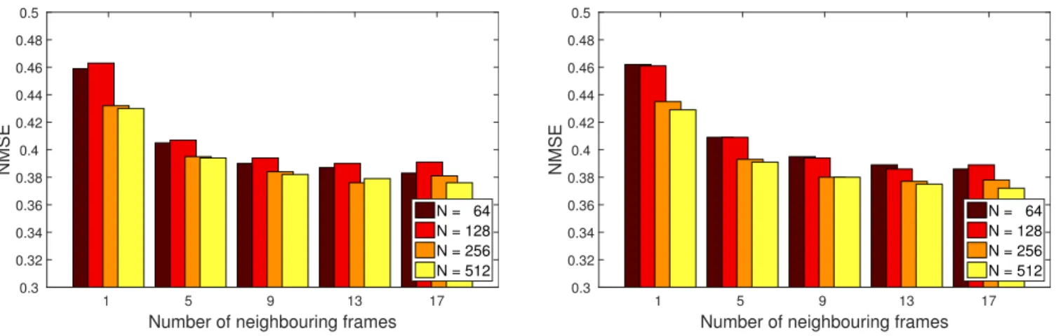
Fig. 4 (left) shows the measured normalized mean squared error scores on the development set for the different, autoencoder network-based configurations. It is clear that, by using

(5)

Number of neighbouring frames

1 5 9 13 17

NMSE

0.3 0.32 0.34 0.36 0.38 0.4 0.42 0.44 0.46 0.48 0.5

N = 64 N = 128 N = 256 N = 512

1 5 9 13 17

NMSE

0.3 0.32 0.34 0.36 0.38 0.4 0.42 0.44 0.46 0.48 0.5

N = 64 N = 128 N = 256 N = 512

Fig. 4. Average NMSE scores measured on the development set (left) and on the test set (right) as a function of the size of the bottleneck layer of the autoencoder network (N) and the number of neighbouring frames used.

1 5 9 13 17

Average correlation

0.7 0.72 0.74 0.76 0.78 0.8

N = 64 N = 128 N = 256 N = 512

1 5 9 13 17

Average correlation

0.7 0.72 0.74 0.76 0.78 0.8

N = 64 N = 128 N = 256 N = 512

Fig. 5. Average Pearson’s correlation scores measured on the development set (left) and on the test set (right) as a function of the size of the bottleneck layer of the autoencoder network (N) and the number of neighbouring frames used.

1 and 5 (2-2) neighbouring frames, we get significantly worse estimates than by using 9 (4-4) frames; when having a larger sliding window size, however, the improvement becomes negligible. Examining the size of the bottleneck layer of the autoencoder network we can see that the networks having N = 64 or N = 128 neurons led to a slightly less precise parameter estimates than withN = 256orN = 512; however, the difference was only significant when we did not use any neighbouring frames. The NMSE scores measured on the test set (see Fig. 4 (right)) display practically the same tendencies as those on the development set.

The mean Pearson’s correlation scores behaved quite similarly both on the development set (see Fig. 5 (left)) and on the test set (Fig. 5 (right)): using 9 (4-4) neighbouring feature vectors led to optimal or close-to-optimal values. We found that it was worth employing at least 256 neurons in the bottleneck layer of the autoencoder network, although the observed difference was probably not significant among the different configurations, at least when we relied on 9 or more neighbouring images.

Examining the actual normalized mean squared error and Pearson’s correlation values (see Table I) we notice that,

when we used the original ultrasound image pixel-by-pixel, the neighbouring frame vectors did not help the prediction for some reason (in our previous studies this was not the case [7]–

[9]). Among the autoencoder-based models we achieved the best performance for both objective evaluation metrics and for both subsets in the N = 256case using 13 (6-6) neighbours;

however, we also see that using only 9 neighbouring frames leads to just slightly worse scores. The NMSE scores of 0.376−0.394 on the test set mean a relative error reduction score of 25-29%, while the0.776−0.787 correlation values brought relative improvements of 30-33% over the0.680score used as the baseline; this improvement is definitely significant.

Table I also lists the size (i.e. the total number of weights) of each DNN model. Of course, for the autoencoder-based models first we have to encode the ultrasound images; therefore, in these cases, the indicated values already contain the size of the encoding part of the autoencoder network (being 0.5 million (N = 64), 1.0 million (N = 128), 2.1 million (N = 256) and 4.2 million (N = 512)). It is quite apparent that the size of the autoencoder-based models only rarely exceed the size of our baseline model (which worked directly on the (resized) ultrasound image), and they were significantly smaller in

(6)

TABLE I

THE AVERAGENMSEAND AVERAGEPEARSON’S CORRELATION COEFFICIENTS MEASURED ON THE DEVELOPMENT AND TEST SETS,AND THE NUMBER OF WEIGHTS OF THE DIFFERENT CONFIGURATIONS TESTED

No. of No. of NMSE Correlation

Technique frames weights Dev. Test Dev. Test

Standard 1 12.6M 0.529 0.534 0.680 0.676

5 46.2M 0.523 0.530 0.684 0.680

Autoencoder. N = 64 1 4.8M 0.459 0.462 0.731 0.729

9 5.3M 0.390 0.395 0.779 0.776

Autoencoder. N = 256

1 6.6M 0.432 0.435 0.750 0.749

9 8.7M 0.384 0.380 0.783 0.786

13 9.7M 0.376 0.377 0.788 0.787

1 8.9M 0.430 0.429 0.751 0.752

Autoencoder. N = 512 5 11.0M 0.394 0.391 0.776 0.778

9 13.1M 0.382 0.380 0.783 0.785

0 20 40 60 80

Mean naturalness

98

13.21 75.16

16.58 15.67 26.04

40.07 40.98

a) Natural b) Anchor c) Vocoded d) Baseline

e) Baseline, 5 images f) AE, N=64, 1 image g)AE, N=256, 9 images h) AE, N=512, 17 images

Fig. 6. Results of the listening test concerning naturalness. The error bars show the 95% confidence intervals.

each case than the DNN working on five consecutive frames.

Based on these scores, we may conclude that the proposed, autoencoder-based approach not only leads to a more accurate estimation of the speech synthesis spectral parameters, but it is also more feasible from a computational viewpoint.

V. SUBJECTIVELISTENINGTESTRESULTS

In order to determine which proposed system is closer to natural speech, we conducted an online MUSHRA (MUlti- Stimulus test with Hidden Reference and Anchor) listening test [55]. The advantage of MUSHRA is that it allows the evaluation of multiple samples in a single trial without break- ing the task into many pairwise comparisons. In the test, the listeners had to rate the naturalness of each stimulus in a randomized order relative to the reference (which was the natural sentence), from 0 (very unnatural) to 100 (very natural). We chose ten sentences from the test set; the variants appeared in randomized order (different for each listener).

Each sentence was rated by 14 native Hungarian speakers.

Our listening test contained utterances synthesized from seven variants of spectral estimates along with the reference recording. Firstly, we used an anchor sentence, which was synthesized from a distorted version of the original MGC-LSP

features (i.e., in analysis-synthesis with the vocoder, the lowest 6 values of the MGC-LSP parameters were used from the original recording, while the higher parameters were constant, resulting in a speech-like but difficult-to-understand lower anchor). The vocoded reference sentences were synthesized by applying impulse-noise excitation using the original F0 and MGC-LSP values of the signals; these utterances correspond to a form of “glass ceiling” for our DNN models, and measure the loss of naturalness due to the speech synthesis (i.e. vocoding) step. Next, we included both variants of the baseline approach in the listening step, i.e. we used the 8 192 pixels of the ultrasound images as features. In the first case, we used only one image as input, while in the second one we concatenated the pixels of five consecutive images. Lastly, we included three autoencoder-based models in the listening test. The first one was the simplest and smallest autoencoder-based model, i.e.N = 64without any neighbouring vectors. As the other extreme case, we tested the variation that had the most parameters, i.e. N = 512 using 8-8 neighbouring frames (17 frames overall). As the last model tested, we chose the one that we found gave practically optimal performance along with a (relatively) small number of parameters:N = 256using 4-4 neighbouring feature vectors on both sides.

Fig. 6 shows the average naturalness scores for these tested approaches. In general, these values are in accordance with the trends we found for the objective measurements.

The standard, pixel-by-pixel approach was the worst DNN- based technique tested, and the subjects did not hear any improvement in the naturalness of the synthesized samples when we used the neighbouring frames as well to assist MGC- LSP prediction. (We would like to note, though, that the synthesized sentences were understandable in each case, even for the anchor approach.) Compared to the baseline scores, using autoencoders for feature extraction brought significant improvements: even the N = 64 case without the help of neighbouring frames led to an average naturalness score of 26.04%. The two further cases included in the listening test, i.e. N = 256 with 9 frames and N = 512 with 17 frames led to even more natural-sounding synthesized utterances; our participants, however, found no significant difference between these two configurations. Of course, there is still room for

(7)

improvement in the quality of the resulting speech samples, as all the models tested produced clearly lower quality utterances than the vocodedone.

VI. CONCLUSIONS

We investigated the applicability of autoencoder neural networks in ultrasound-based speech silent interfaces. In the proposed approach, we used the activations of the bottleneck layer of the autoencoder network as features, and we estimated the MGC-LSP parameters of the speech synthesis step via a second deep network. According to our experimental results, the proposed autoencoder-based process is a more viable approach than the baseline one, which treats each pixel as an independent feature: the estimations were more accurate in every case, and the DNN model had fewer weights as well. Our listening tests also demonstrated the benefit of using autoencoder-based compression.

In our opinion, this improvement is mainly due to two fac- tors. Firstly, the autoencoder network automatically performs a de-noising step on the input ultrasound image; as ultrasound videos are quite noisy by nature, a de-noising step might help in the location of the tongue and the lips, thus allowing more precise spectral parameter estimation. The second advantage of our process is that the autoencoder network also performs a compression of the original image. Using the activations of the bottleneck layer significantly reduced the size of our feature vector, which allowed us to estimate the spectral speech synthesis parameters using more consecutive images (i.e. a larger sliding window size) without relying on an unrealistically huge feature vector.

We have several straightforward possibilities for continuing our experiments. We could combine the autoencoder network with convolutional neural networks, which will hopefully improve the efficiency of the proposed procedure even more.

An autoencoder-based process can be also expected to tolerate slight changes in the recording equipment position more than the baseline approach, where we treat all pixels as independent features. Therefore, utilizing the encoder part of the autoencoder network for feature extraction might contribute to the development of more session-independent and speaker- independent silent speech interface systems. We also plan to perform these kinds of experiments in the near future.

ACKNOWLEDGMENTS

László Tóth was supported by the János Bolyai Research Scholarship of the Hungarian Academy of Sciences and the UNKP-18-4 New Excellence Program of the Hungarian Min- istry of Human Capacities. Tamás Grósz was supported by the National Research, Development and Innovation Office of Hungary through the Artificial Intelligence National Excel- lence Program (grant no.: 2018-1.2.1-NKP-2018-00008). We acknowledge the support of the Ministry of Human Capacities, Hungary grant 20391-3/2018/FEKUSTRAT. The authors were partially funded by the NKFIH FK 124584 grant and by the MTA Lendület program. The Titan X graphics card used in this research was donated by the Nvidia Corporation. We would

also like to thank the subjects who participated in the listening test.

REFERENCES

[1] B. Denby, T. Schultz, K. Honda, T. Hueber, J. M. Gilbert, and J. S.

Brumberg, “Silent speech interfaces,” Speech Communication, vol. 52, no. 4, pp. 270–287, 2010.

[2] B. Denby and M. Stone, “Speech synthesis from real time ultrasound images of the tongue,” in Proc. ICASSP, Montreal, Quebec, Canada, 2004, pp. 685–688, IEEE.

[3] Bruce Denby, Jun Cai, Thomas Hueber, Pierre Roussel, G´erard Dreyfus, Lise Crevier-Buchman, Claire Pillot-Loiseau, G´erard Chollet, Sotiris Manitsaris, and Maureen Stone, “Towards a Practical Silent Speech Interface Based on Vocal Tract Imaging,” in9th International Seminar on Speech Production (ISSP 2011), 2011, pp. 89–94.

[4] Thomas Hueber, Elie-Laurent Benaroya, G´erard Chollet, G´erard Drey- fus, and Maureen Stone, “Development of a silent speech interface driven by ultrasound and optical images of the tongue and lips,”Speech Communication, vol. 52, no. 4, pp. 288–300, 2010.

[5] Thomas Hueber, Elie-laurent Benaroya, Bruce Denby, and G´erard Chol- let, “Statistical Mapping Between Articulatory and Acoustic Data for an Ultrasound-Based Silent Speech Interface,” in Proc. Interspeech, Florence, Italy, 2011, pp. 593–596.

[6] Aurore Jaumard-Hakoun, Kele Xu, Cl´emence Leboullenger, Pierre Roussel-Ragot, and Bruce Denby, “An Articulatory-Based Singing Voice Synthesis Using Tongue and Lips Imaging,” inProc. Interspeech, 2016, pp. 1467–1471.

[7] Tamás Gábor Csapó, Tamás Grósz, Gábor Gosztolya, László Tóth, and Alexandra Markó, “DNN-based ultrasound-to-speech conversion for a Silent Speech Interface,” in Proceedings of Interspeech, Stockholm, Sweden, Aug 2017, pp. 3672–3676.

[8] Tamás Grósz, Gábor Gosztolya, László Tóth, Tamás Gábor Csapó, and Alexandra Markó, “F0 estimation for DNN-based ultrasound silent speech interfaces,” inProceedings of ICASSP, Calgary, Alberta, Canada, Apr 2018, pp. 291–295.

[9] László Tóth, Gábor Gosztolya, Tamás Grósz, Alexandra Markó, and Tamás Gábor Csapó, “Multi-task learning of speech recognition and speech synthesis parameters for ultrasound-based silent speech interfaces,” inProceedings of Interspeech, Hyderabad, India, Sep 2018, pp.

3172–3176.

[10] Kele Xu, Pierre Roussel, Tamás Gábor Csapó, and Bruce Denby, “Con- volutional neural network-based automatic classification of midsagittal tongue gestural targets using B-mode ultrasound images,” The Journal of the Acoustical Society of America, vol. 141, no. 6, pp. EL531–EL537, 2017.

[11] Eric Tatulli and Thomas Hueber, “Feature extraction using multimodal convolutional neural networks for visual speech recognition,” inProc.

ICASSP, 2017, pp. 2971–2975.

[12] Jun Wang, Ashok Samal, Jordan R Green, and Frank Rudzicz, “Sentence Recognition from Articulatory Movements for Silent Speech Interfaces,”

inProc. ICASSP, 2012, pp. 4985–4988.

[13] Jun Wang, Ashok Samal, and Jordan Green, “Preliminary Test of a Real-Time, Interactive Silent Speech Interface Based on Electromagnetic Articulograph,” in Proceedings of the 5th Workshop on Speech and Language Processing for Assistive Technologies, 2014, pp. 38–45.

[14] Florent Bocquelet, Thomas Hueber, Laurent Girin, Christophe Savari- aux, and Blaise Yvert, “Real-Time Control of an Articulatory-Based Speech Synthesizer for Brain Computer Interfaces,” PLOS Computa- tional Biology, vol. 12, no. 11, pp. e1005119, nov 2016.

[15] Myungjong Kim, Beiming Cao, Ted Mau, and Jun Wang, “Speaker- Independent Silent Speech Recognition From Flesh-Point Articulatory Movements Using an LSTM Neural Network,”IEEE/ACM Transactions on Audio, Speech, and Language Processing, vol. 25, no. 12, pp. 2323–

2336, dec 2017.

[16] Beiming Cao, Myungjong Kim, Jun R Wang, Jan Van Santen, Ted Mau, and Jun Wang, “Articulation-to-Speech Synthesis Using Articulatory Flesh Point Sensors’ Orientation Information,” in Proc. Interspeech, Hyderabad, India, 2018, pp. 3152–3156.

[17] Fumiaki Taguchi and Tokihiko Kaburagi, “Articulatory-to-speech conversion using bi-directional long short-term memory,” in Proc. Inter- speech, Hyderabad, India, 2018, pp. 2499–2503.

(8)

[18] M. J. Fagan, S. R. Ell, J. M. Gilbert, E. Sarrazin, and P. M. Chapman,

“Development of a (silent) speech recognition system for patients following laryngectomy,” Medical Engineering and Physics, vol. 30, no. 4, pp. 419–425, 2008.

[19] Jose A. Gonzalez, Lam A. Cheah, Angel M. Gomez, Phil D. Green, James M. Gilbert, Stephen R. Ell, Roger K. Moore, and Ed Holdsworth,

“Direct Speech Reconstruction From Articulatory Sensor Data by Ma- chine Learning,” IEEE/ACM Transactions on Audio, Speech, and Language Processing, vol. 25, no. 12, pp. 2362–2374, dec 2017.

[20] Keigo Nakamura, Matthias Janke, Michael Wand, and Tanja Schultz,

“Estimation of fundamental frequency from surface electromyographic data: EMG-to-F0,” inProc. ICASSP, Prague, Czech Republic, 2011, pp.

573–576.

[21] Yunbin Deng, James T. Heaton, and Geoffrey S. Meltzner, “Towards a practical silent speech recognition system,” in Proc. Interspeech, Singapore, Singapore, 2014, pp. 1164–1168.

[22] Lorenz Diener, Matthias Janke, and Tanja Schultz, “Direct conversion from facial myoelectric signals to speech using Deep Neural Networks,”

in2015 International Joint Conference on Neural Networks (IJCNN).

jul 2015, pp. 1–7, IEEE.

[23] Matthias Janke and Lorenz Diener, “EMG-to-Speech: Direct Generation of Speech From Facial Electromyographic Signals,” IEEE/ACM Trans- actions on Audio, Speech, and Language Processing, vol. 25, no. 12, pp. 2375–2385, dec 2017.

[24] Geoffrey S. Meltzner, James T. Heaton, Yunbin Deng, Gianluca De Luca, Serge H. Roy, and Joshua C. Kline, “Silent speech recognition as an alternative communication device for persons with laryngectomy,”

IEEE/ACM Transactions on Audio Speech and Language Processing, vol. 25, no. 12, pp. 2386–2398, 2017.

[25] Lorenz Diener, Gerrit Felsch, Miguel Angrick, and Tanja Schultz,

“Session-Independent Array-Based EMG-to-Speech Conversion using Convolutional Neural Networks,” in13th ITG Conference on Speech Communication, 2018.

[26] Michael Wand, Tanja Schultz, Istituto Dalle, and Intelligenza Artificiale,

“Domain-Adversarial Training for Session Independent EMG-based Speech Recognition,” Hyderabad, India, 2018, pp. 3167–3171.

[27] Neil Shah, Nirmesh Shah, and Hemant Patil, “Effectiveness of Genera- tive Adversarial Network for Non-Audible Murmur-to-Whisper Speech Conversion,” inProc. Interspeech, Hyderabad, India, 2018, pp. 3157–

3161, ISCA.

[28] João Freitas, Artur J Ferreira, Mário A T Figueiredo, António J S Teixeira, and Miguel Sales Dias, “Enhancing multimodal silent speech interfaces with feature selection,” in Proc. Interspeech, Singapore, Singapore, 2014, pp. 1169–1173.

[29] Michael Wand, Jan Koutn´ık, and J¨urgen Schmidhuber, “Lipreading with long short-term memory,” inProc. ICASSP, Shanghai, China, 2016, pp.

6115–6119.

[30] Tanja Schultz, Michael Wand, Thomas Hueber, Dean J. Krusienski, Christian Herff, and Jonathan S. Brumberg, “Biosignal-Based Spoken Communication: A Survey,”IEEE/ACM Transactions on Audio, Speech, and Language Processing, vol. 25, no. 12, pp. 2257–2271, dec 2017.

[31] Geoffrey Hinton, Li Deng, Dong Yu, George Dahl, Abdel-rahman Mohamed, Navdeep Jaitly, Andrew Senior, Vincent Vanhoucke, Patrick Nguyen, Tara Sainath, and Brian Kingsbury, “Deep Neural Networks for Acoustic Modeling in Speech Recognition: The Shared Views of Four Research Groups,” IEEE Signal Processing Magazine, vol. 29, no. 6, pp. 82–97, nov 2012.

[32] Zhen-Hua Ling, Shi-Yin Kang, Heiga Zen, Andrew Senior, Mike Schus- ter, Xiao-Jun Qian, Helen Meng, and Li Deng, “Deep Learning for Acoustic Modeling in Parametric Speech Generation,” IEEE Signal Processing Magazine, vol. 32, no. 3, pp. 35–52, 2015.

[33] Ebru Arisoy, Tara N Sainath, Brian Kingsbury, and Bhuvana Ramabhad- ran, “Deep Neural Network Language Models,” inProceedings of the NAACL-HLT 2012 Workshop: Will We Ever Really Replace the N-gram Model? On the Future of Language Modeling for HLT, 2012, WLM

’12, pp. 20–28.

[34] Zheng-Chen Liu, Zhen-Hua Ling, and Li-Rong Dai, “Articulatory-to- acoustic conversion with cascaded prediction of spectral and excitation features using neural networks,” inProc. Interspeech, 2016, pp. 1502–

1506.

[35] Cenxi Zhao, Longbiao Wang, Jianwu Dang, and Ruiguo Yu, “Prediction of F0 based on articulatory features using DNN,” inProc. ISSP, Tienjin, China, 2017.

[36] Ian Goodfellow, Jean Pouget-Abadie, Mehdi Mirza, Bing Xu, David Warde-Farley, Sherjil Ozair, Aaron Courville, and Yoshua Bengio,

“Generative Adversarial Nets,” in Advances in Neural Information Processing Systems 27 (NIPS 2014), 2014, pp. 2672–2680.

[37] Maureen Stone, B Sonies, T Shawker, G Weiss, and L Nadel, “Analysis of real-time ultrasound images of tongue configuration using a grid- digitizing system,” Journal of Phonetics, vol. 11, pp. 207–218, 1983.

[38] Maureen Stone, “A guide to analysing tongue motion from ultrasound images,”Clinical Linguistics & Phonetics, vol. 19, no. 6-7, pp. 455–501, jan 2005.

[39] Tamás Gábor Csapó and Steven M Lulich, “Error analysis of extracted tongue contours from 2D ultrasound images,” in Proc. Interspeech, Dresden, Germany, 2015, pp. 2157–2161.

[40] David E. Rumelhart, Geoffrey E. Hinton, and Ronald J. Williams,

“Learning internal representations by error propagation,” in Parallel Distributed Processing: Explorations in the Microstructure of Cognition, Volume 1: Foundations, pp. 318–362. MIT Press, Cambridge, MA, 1986.

[41] Stefan Lattner, Maarten Grachten, and Gerhard Widmer, “Learning transformations of musical material using Gated Autoencoders,” in Proceedings of CSMC, Milton Keynes, United Kingdom, Sep 2017, pp.

1–16.

[42] Krzysztof J. Geras and Charles Sutton, “Scheduled denoising autoencoders,” in Proceedings of ICLR, San Diego, USA, May 2015, pp.

365–368.

[43] Zhengxue Cheng, Heming Sun, Masaru Takeuchi, and Jiro Katto,

“Deep convolutional autoencoder-based lossy image compression,” in Proceedings of PCS, San Francisco, USA, June 2018, pp. 253–257.

[44] Shengjia Zhao, Jiaming Song, and Stefano Ermon, “Learning hierarchi- cal features from generative models,” inProceedings of ICML, Sydney, Australia, Aug 2017, pp. 4091–4099.

[45] Dongdong Chen, Lu Yuan, Jing Liao, Nenghai Yu, and Gang Hua,

“StyleBank: An explicit representation for neural image style transfer,”

inProceedings of CVPR, Honolulu, Hawaii, July 2017.

[46] Martin Andrews, “Compressing word embeddings,” inProceedings of ICONIP, Kyoto, Japan, Oct 2016, pp. 413–422.

[47] Naftali Tishby and Noga Zaslavsky, “Deep learning and the information bottleneck principle,” inProceedings of ITW, Jerusalem, Israel, April 2015, pp. 1–5.

[48] Arturo Camacho and John G Harris, “A sawtooth waveform inspired pitch estimator for speech and music,” The Journal of the Acoustical Society of America, vol. 124, no. 3, pp. 1638–1652, Sep 2008.

[49] Keiichi Tokuda, Takao Kobayashi, Takashi Masuko, and Satoshi Imai,

“Mel-generalized cepstral analysis – a unified approach to speech spectral estimation,” inProceedings of ICSLP, Yokohama, Japan, 1994, pp. 1043–1046.

[50] Satoshi Imai, Kazuo Sumita, and Chieko Furuichi, “Mel log spectrum approximation (MLSA) filter for speech synthesis,” .

[51] L´aszl´o Varga, Information Content of Projections and Reconstruction of Objects in Discrete Tomography, Ph.D. thesis, Doctoral School of Computer Science, University of Szeged, 2013.

[52] Mart´ın Abadi, Ashish Agarwal, Paul Barham, Eugene Brevdo, Zhifeng Chen, Craig Citro, Greg S. Corrado, Andy Davis, Jeffrey Dean, Matthieu Devin, Sanjay Ghemawat, Ian Goodfellow, Andrew Harp, Geoffrey Irving, Michael Isard, Yangqing Jia, Rafal Jozefowicz, Lukasz Kaiser, Manjunath Kudlur, Josh Levenberg, Dandelion Man´e, Rajat Monga, Sherry Moore, Derek Murray, Chris Olah, Mike Schuster, Jonathon Shlens, Benoit Steiner, Ilya Sutskever, Kunal Talwar, Paul Tucker, Vin- cent Vanhoucke, Vijay Vasudevan, Fernanda Vi´egas, Oriol Vinyals, Pete Warden, Martin Wattenberg, Martin Wicke, Yuan Yu, and Xiaoqiang Zheng, “TensorFlow: Large-scale machine learning on heterogeneous systems,” 2015, Software available from tensorflow.org.

[53] Prajit Ramachandran, Barret Zoph, and Quoc V. Le, “Searching for activation functions,” inProceedings of ICLR, 2018, p. submitted.

[54] Stefan Elfwing, Eiji Uchibe, and Kenji Doya, “Sigmoid-weighted linear units for neural network function approximation in reinforcement learning,”Neural Networks, vol. 107, pp. 3–11, 2018.

[55] “ITU-R recommendation BS.1534: Method for the subjective assessment of intermediate audio quality,” 2001.