An ANN-based Speed and Flux Controller of Three-Phase AC Motors with Uncertain Parameters

An ANN-based Speed and Flux Controller of Three-Phase AC Motors with Uncertain Parameters

Hung Linh Le

Faculty of Automation Technology, University of Information and Communication Technology, Thai Nguyen University

Quyet Thang, Thai Nguyen, Vietnam lhlinh@ictu.edu.vn

Thuong Cat Pham

Institute of Information Technology, Vietnam Academy of Science and Technology

18, Hoang Quoc Viet, Hanoi, Vietnam ptcat@ioit.ac.vn

Minh Tuan Pham

Space Technology Institute, Vietnam Academy of Science and Technology 18, Hoang Quoc Viet, Hanoi, Vietnam

pmtuan@sti.vast.vn

Abstract: This paper proposes a speed and flux control method of three-phase AC motors using an artificial neural network (ANN) to compensate for uncertain parameters in the motor’s dynamic model such as rotor resistance, moment of inertia, friction coefficients, and load changes during system operation. Global asymptotic stability of the overall system is proved by Lyapunov’s theory. Matlab simulation results are given to demonstrate the validity of the proposed control method.

Keywords: three-phase AC motor; artificial neural network; speed and flux control;

uncertain dynamics

1 Introduction

AC motor speed control has been a popular topic over the past decades, because of uncertain parameters in the system model such as rotor resistance, flux, friction coefficient and variable load [1][2][3][9]. Recently, to estimate motor speed without using speed sensors, many researchers utilize Kalman filters or sliding mode observers [8][9]. These would help reduce production costs. However, the control performance would rely heavily on the estimation algorithm and the accuracy of motor model. The classical control method cannot obtain effective control, when the load of the system changes gradually due to uncertain parameters in the dynamic model of the AC motor. In this case, self-adaptive control [4][5][6][7], on-line identification methods and controllers with neural networks were used.

The main focus of recent research has been to determine a control algorithm and estimate the motor speed based on rotor flux orientation. In this method, the speed of the flux vector is controlled to reach the synchronous speed. Thus, the AC motor speed control is the same as the structure of DC motor control [11][12]. The main objective was to decouple two currents i_sd, i_sqindependently. However, these two currents interact and depend on synchronous speed w_s. Therefore, this method operates well in static mode and indicates clearly when the system operates in the flux declining domain. This paper proposes a method of speed and flux control for AC motors using an artificial neural network to compensate for uncertain parameters in the dynamic model, such as rotor resistance, moment, friction coefficient as well as a variable load during system operation.

The paper is organized as follows. The second section discusses the speed and flux control models for AC motors. The third section shows the speed and flux control methods with uncertain parameters. The last section presents simulations to verify the efficiency of the proposed method.

2 Speed and Flux Control Model for AC Motors

Table 1 Nomenclature

Notion Unit Meaning

M, N, D, Q Model Matrices

B Nms/rad Friction coefficient

J Nms²/rad Inertia moment of rotor

TL Nm Load torque

s, r

R R _Ω Stator and rotor resistance

s, r

L L H Stator and rotor inductance

Lm H Inductance between stator winding and rotor winding

ref,

w w Rad/s Reference angular velocity, rotor angular velocity

ra, rb

y y Wb Horizontal and vertical parts of rotor flux

r ,r

i_a i_{b A} Horizontal and vertical components of rotor current

r , r

u_a u_b V Horizontal and vertical components of rotor voltage Consider a dynamic model of a three phase motor with a squirrel-cage rotor as follows:

1

1

s s r r

m s r r

s r r s

s s r r

m s r r

s r r s

r r r

r r m s

r r

r r r

r r m s

r r

di R R R

L i u

dt L L L L

di R R R

L i u

dt L L L L

d R R

dt L L L i

d R R

dt L L L i

a a a b a

b

b a b b

a a b a

b a b b

b b y bwy

s s

b bwy b y

s s

y y wy

y wy y

  

 

  

       

  

  

  

 

       

  

  

  

    



  





(1)

 

L r s r s

Jd B T K i i

dt ^{a b b a}

w w  y y (2)

where

2

1 ^m

s r

L

s L L ; ^m

s r

L b L L

s ; 3

2

m r

P L

K L is the moment coefficient. L_s,L_r, Lm and R_s rarely change and can be measured accurately. However, rotor resistance R_r often changes in accordance with motor temperature during operation.

The principle goal of this paper is to determine control signals u_sa,u_sb to regulate the speed and flux of the motor reach these desired values ww_ref^,

 

2 2 2 2

ref

r ra rb r

y  y y y ^{, where} R J B_r, , andT_L are unknown.

Assuming that i_sa,i_sb are known and motor speed w can be measured or estimated, taking the derivative of equation (2), we obtain:

 

L r s r s r s r s

JwBwT K y_{a b}i y_{a b}i y_{b a}i y_{b a}i (3) Substituting equation (1) into (3) and setting x₁w yields the speed equation:

 

   

   

1 1 1

2 2

1

1

L r s r s

s r

m r s r s

s r

r r r r

s

Jx Bx T Kx i i

R R

K L i i

L L

K x K u u

L

a a b b

a b b a

a b a b b a

y y

b y y

s

b y y y y

s

    

 

 

     

   

  

(4)

By setting x₂ y_r²_ay_r²_b, the flux equation can be written as:

 

   

 

 

2

2 2

2 2

1 2

2

2 2

2 1

2

2 2

r r

m s s

r r

s

r r

m m r r r r

r s r

r

m r s r s

r

r m

r

m r r

r r s

R R

x x L i i

L L

R

R R

L L i i

L L L

R L x i i

L

R L

R L x u u

L L L

a b

a a b b

a b b a

a a b b

b y y

s

y y

b y y

s

  

       

 

 

     

 

  

      

 

(5)

From equation (4) and (5), we obtain a state equation:

xMx + Nx Q D u^1

  (6)

where x



x1 x2



^T; u u_a u_b^T



¹



⁰

0 2

M

s r

m

s r

r r

R R

B L

J L L

R L s b

 

    

 

 

  

 

2

1 0

0 2

s r

m

s r

r m r

R R

B L

J L L

R L L s b

b

   

     

   

 

         N

  _{ }

   

   

1 1 2

2

2 2

1

1

2 1

2 2

r s r s s r L L

m

s r

s

r r

m m r r r r

r s r

r r

m r s r s m s s

r r

Kx i i K x x R R T T

J J L L L J J

R

R R

L L i i

L L L

R R

L x i i L i i

L L

a a b b

a a b b

a b b a a b

y y b b

s

b y y

s

y y

    

       

   

 

 

   

       

             Q



1 1

2 2

r r

r m r m

s r r

r r

K K

J J

R L R L

L

L L

b a

a b

y y

s y y



 

  

 

 

  

 

 

 

D

B, J, R_r and variable load T_Lare uncertain parameters such as:

ˆ

r ˆr r

B B B

J J J

R R R

 

 

 



ˆ ˆ ˆ, , _r

B J R are known parameters.

, , _r

J B R

   are unknown parameters.

From known parameters, the components of flux y yˆ_ra,ˆ_rb can be determined following the equation:

ˆ ˆ ˆ

ˆ ˆ

ˆ ˆ ˆ

ˆ ˆ

r r r

r r m s

r r

r r r

r r m s

r r

d R R

dt L L L i

d R R

dt L L L i

a a b a

b

a b b

y y wy

y wy y

    



   



(7)

Matrices in equation (6) can be represented as follows:

ˆ ; ˆ

ˆ ; ˆ

N = N +ΔN M = M + ΔM

Q = Q +ΔQ D = D + ΔD (8)

where Q D M N are known matrices;ˆ ˆ ˆ, , ,ˆ   Q, D, M,N are unknown.

 

ˆ ˆ

1 0

ˆ ˆ

ˆ

0 2

s r

m

s r

r r

R R

B L

L L

J

R L s b

 

    

 

 

   M

 

2

ˆ ˆ

1 0

ˆ ˆ

ˆ

0 2

s r

m

s r

r m r

R R

B L

L L

J

R L

L s b

b

   

     

   

   

 

          N

   

 

 

   

2 2

1 1

2

2 2

1

ˆ ˆ ˆ ˆ

ˆ ˆ

ˆ ˆ

ˆ ˆ

ˆ 2 1

ˆ ˆ

ˆ ˆ

2 2

r s r s r r

s

r r

m m r r r r

r s r

r r

m r s r s m s s

r r

Kx i i K x

J J

R

R R

L L i i

L L L

R R

L x i i L i i

L L

a a b b a b

a a b b

a b b a a b

y y b y y

b y y

s

y y

    

 

  

 

 

   

      

           Q



^{2 2}



ˆ ˆ ˆ

ˆ 2 ˆ

ˆ

ˆ

ˆ ˆ

2 ˆ 2 ˆ ˆ

ˆ

r m

r r

s r r

r m

m r r r

r r

r

R L K

L L J L J

R L

KL R K

L J

D

b a

a b

a b

y y

s

y y y y

 

 

 

 

   

Let us choose



^ˆ



uD vˆ Q ⁽⁹⁾

with v v_a v_b^T being an augmented control signal.

Substituting equation (9) into (6) we obtain:

ˆ ˆ

v x Mx + Nx f (10)

with f =ΔMx + ΔNx D^1DvD^1DQˆQ being an unknown element that can be estimated later.

In summary, the motor control problem becomes determining the control signal v that regulates motor speed and motor flux reach their respective desired values wwref^{, yr2 }



^yr2ayr2b



^{yr2ref where J B R, , r} and changeable load T_L are unknown.

3 Speed and Flux Control Method for AC Motors with Uncertain Parameters

We denote:

s = e + Ce (11)

where C is the positive definite diagonal matrix; e x x_ref is the error between the actual value x



x1 x2



^T w yr²^T

and the desired value xref 



x1ref x2ref



^T wref yr²ref^T. Therefore, when , then e0.

From equation (10), f is an unknown function which includes physical motor parameters such as flux, current, voltage and speed. However, in practice the variation of these parameters can be considered bounded and continuous. The motor speed and flux are bounded quantities, so f is also bounded and continuous:

fmax

f  . The solution is to determine the control signal v which drives error e to approach 0 when lim ( )

t t

e 0 without knowing f exactly. This corresponds to finding the control signal v assuring lim ( )

t t

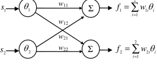
s 0 . Applying the universal approximation capacity of artificial neural networks for continuous, bounded unknown nonlinear functions, we can use an artificial neural network with self- adaptation to approximate the unknown parameter f of system (10) based on known signal s(t). From [10], the artificial neural network structure is an RBF network. We chose a RBF network as seen in Figure 1 with two inputs, two outputs and three layers to approximate f. The input layer of the neural network consists of the two elements of s(t) and the output layer has two linear neurons.

The hidden layer is composed of two neurons having the following Gauss distribution function:

 

²

exp ^j 2 ^j ; 1, 2

j

j

s c q j

l

 

  

 

   

where c_j,_jare the expectation and variance of the Gaussian distribution function that are freely chosen.

Figure 1 The neural network structure The form of the neural network:

f  fˆ ε Wθε (12)

 s 0

s

1



₁



2

w₁₁

Σ

w₂₂ w₁₂ w₂₁

2

Σ s

2

2 2

1 i i i

f w 

=

= ∑

2

1 1

1 i i i

f w 

=

= ∑

where ^{11 12}

21 22

w w w w

 

 

  

W is a weighted matrix;



1 2



^T

θ q q is an output function vector of input neuron;

ε is a bounded approximation error ε e₀.

Therefore, to make s0 and error e0, we need to choose v and the learning rule for the weighted W to make the system (10) asymptotically stable.

Theorem: Speed and flux of the AC motor in equation (2) approach the desired values ww_ref ^{and yr2}



^yr2ayr2b



^{yr2ref while J, B, Rr} and changeable load T_L are unknown if the control signal v and weighted W are defined as below:

ˆ ˆ ref

v HsMxNxx Cev1 (13)

 

1 1 s

v Wθ

m g s

   (14)

w_im qs _i (15)

where H is a positive definite diagonal matrix, w_i is the i^th column of the weighted matrix W, m0 and g e r ₀ ^with r0.

Proof:

Applying Lyapunov’s stability theory, we chose a positive definite function V such as:

2

T T

1

1 1

2s s 2 w w_{i i}

i

V



 



⁽¹⁶⁾

Taking the derivative of both sides of the equation (16) yields:

2

T T

1

s s w w_{i i}

i

V



 



   (17)

Substituting derivatives ,s w  into (17) yields:

 

 

T T

ref ref

s x x C x x w_{i i}s

i

V^ ^{ }  ^{ } m



q ⁽¹⁸⁾

From equation (10), (12), (13) and (18), we obtain:

 

T T

1 1

s Hs s v Wθ ε

V     m   (19)

Substituting equation (14) into (19), results in:

 

T

T T

T T

0

T T

0

. .

0

V s s

s Hs s ε

s

s Hs s s ε s Hs s s

s Hs s s Hs s

g

g g e

g e r

   

       

       



(20)

It is clear that V0 _when s0 and V0 if and only if s0. Following Lyapunov’s theory, we have s0 and error e0. Therefore, xx_ref. In other words, rotor speed and flux converge to their respective desired values with error e0^.

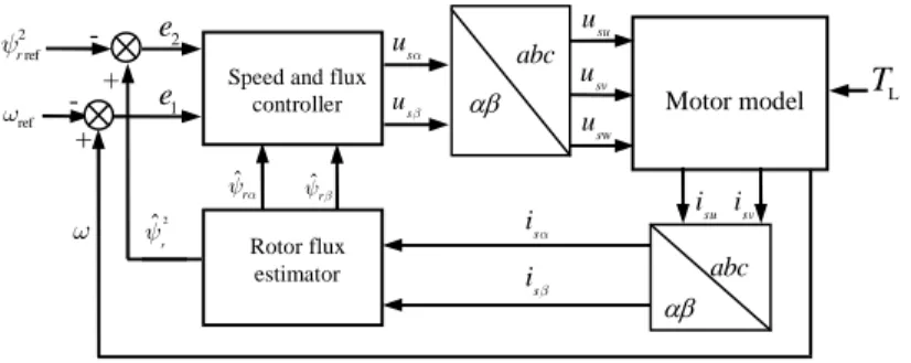
Figure 2 shows the overall motor control system.

Figure 2

The overall motor control system

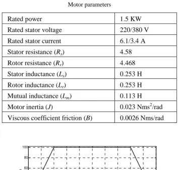
4 Simulation

Simulation was conducted using a four-pole squirrel-cage induction motor from LEROY SOMER with the parameters shown in Table 2. The reference angular velocity w_ref varies in a trapezoid shape as seen in Figure 3 with the maximum speed w_ref 100 (rad/s) and reference flux ^{yr2ref 2.25 Wb}



²



^.

Motor model

Rotor flux estimator Speed and flux

controller

e2

TL

+ e1

+

us_b

us_a

w

us

usv 2

ref

yr

ˆ2

yr

w

ˆra

y y^ˆrb

-

abc



abc



wref

isu i_sv is_a

is_b

usu

- -

Table 2 Motor parameters

Rated power 1.5 KW

Rated stator voltage 220/380 V

Rated stator current 6.1/3.4 A

Stator resistance (Rs) 4.58Ω Rotor resistance (R_r) 4.468Ω Stator inductance (L_s) 0.253 H Rotor inductance (Lr) 0.253 H Mutual inductance (Lm) 0.113 H

Motor inertia (J) 0.023 Nms²/rad

Viscous coefficient friction (B) 0.0026 Nms/rad

Figure 3 Desired rotor speed w_ref

The motor speed control system was simulated with these assumed uncertain parameters:

 



²



ˆ ; ˆ 0.85 ; 0.15 Nms/r

ˆ ; ˆ 0.85 ; 0

ad Nms /rad .15

B B B B B B B

J J J J J J J

     

     

When the unknown changeable load was formulated as ˆ ; 1.5 sin(2 ) 0.5 sin(50 )

L L L L

T T  T  T t  t (Nm)

TL had an amplitude change over time as seen in Figure 4a) and b).

0 5 10 15 20 25 30 35 40 45 50

0 20 40 60 80 100

Time (s)

Rad/s

Figure 4

Simulation with control signal using neural networks and direct rotor speed feedback signal:

a) Load changes suddenly; b) LoadT changes_L The coefficients of the neural network were calculated as follows:

20, _j 0.5,c_j 0.001, 300 m l   g

200 0 0 200, H  

200 0 0 200 C  

The simulation results are shown in Figure 5 to Figure 9.

Based on the simulation results using the neural network shown in Figure 5 to Figure 7, rotor speed and rotor flux were close to the desired values. When the load changed suddenly while the motor was operating normally, speed and rotor flux had a transient period with an error of about 1.6% to rotor angular velocity and 0.1% to rotor flux. Then, they converged rapidly to the desired speed and flux.

The results without using the neural network (v₁= 0) are seen in Figure 8 and Figure 9 which show that rotor speed and flux could not be maintained close to desired values at times when load changed suddenly. Error of rotor angular velocity was about 1.6% and that of the rotor flux about 0.5%.

This proves that the self-adaptive capacity of the system and the efficiency of the proposed control method using ANN with an online learning algorithm compensated for the impact of uncertain parameters and load changes.

a)

b) ^{-20 5 10 15 20 25 30 35 40 45 50}

0 2 4 6 8 10

Time(s)

Nm

Figure 5 Real rotor speedw

Figure 6

Error e1between desired rotor speed w_ref and real rotor speed w

Figure 7

Error e2between desired flux y_r²_ref and estimated flux y_r²

Figure 8

Error e1between desired rotor speed w_ref and real rotor speedw ^when v10

0 5 10 15 20 25 30 35 40 45 50

0 20 40 60 80 100

Time (s)

Rad/s

0 5 10 15 20 25 30 35 40 45 50

-1 -0.5 0 0.5 1

Time (s)

Rad/s

0 5 10 15 20 25 30 35 40 45 50

-5 0 5 x 10^-3

Time (s)

Wb2

0 5 10 15 20 25 30 35 40 45 50

-0.8 -0.6 -0.4 -0.2 0 0.2 0.4 0.6

Time (s)

Rad/s

Figure 9

Error e2between desired fluxy_r²_ref and estimated fluxy_r^{2 when} v10 Conclusion

This paper proposes an adaptive, non-decoupling control method based on an ANN, for speed and flux control of AC motors, with uncertain parameters. Global asymptotic stability of the overall control system is provenby Lyapunov’s direct method. The proposed speed and flux control method performs well while friction, moment of inertia, unknown rotor resistance and load change significantly in the AC motor dynamic model. The simulation results clearly show the efficiency of the proposed method.

References

[1] W. Leonhard, Control of Electric Drives, Springer Verlag, 2001 [2] P. Krause, Analysis of Electric Machinery, McGrawHill, 1986

[3] R. J. Wai, Robust Decoupled Control of Direct Field-oriented Induction Motor Drive, IEEE Transactions on Industrial Electronics, Vol. 52, No. 3, Jun. 2005

[4] S. Rao, M. Buss, and V. Utkin, An Adaptive Sliding Mode Observer for Induction Machines, Proceedings of the 2008 American Control Conference, Seattle, Washington, USA, Jun. 2008, pp. 1947-1951

[5] R. Marino, S. Peresada, and P. Valigi, Adaptive Input Output Linearizing Control of Induction Motors, IEEE Transactions on Automatic Control, Vol. 38, No. 2, Feb. 1993, pp. 208-221

[6] V. I. Utkin, J. G. Guldner, and J. Shi, Sliding Mode Control in Electromechanical Systems. Taylor & Francis, 1999

[7] K. Halbaoui, D. Boukhetala, and F. Boudjema, A New Robust Model Reference Adaptive Control for Induction Motor Drives Using a Hybrid Controller, Proceedings of the International Symposium on Power Electronics, Electrical Drives, Automation and Motion, Jun. 2008, Italy, pp.

1109-1113

0 5 10 15 20 25 30 35 40 45 50

-5 0 5 x 10^-3

Time (s)

Wb2

[8] Z. Yan and V. Utkin, Sliding Mode Observers for Electric Machines an Overview, Proceedings of the IECON 02, Vol. 3, No. 2, MeliáLebreros Hotel, Sevilla, Spain, Nov. 2002, pp. 1842-1847

[9] Derdiyok, Z. Yan, M. Guven, and V. Utkin, A Sliding Mode Speed and Rotor Time Constant Observer for Induction Machines, Proceedings of the IECON 01 (The 27^thAnnual Conference of the IEEE Industrial Electronics Society), Vol. 2, Hyatt Regency Tech Center, Denver, Colorado, USA, Nov. 2001, pp. 1400-1405

[10] N.E Cotter, The Stone-Weierstrass and Its Application to Neural Networks, IEEE Trans. on Neural Networks, Vol. 1, No. 4, 1990, pp. 290-295

[11] P. Marino, M. Milano, F. Vasca, Linear Quadratic State Feedback and Robust Neural Network Estimator for Field-Oriented-Controlled Induction Motors, IEEE Trans. Ind. Electron, Vol. 46, No. 1, 1999, pp. 150-161 [12] Pham Thuong Cat, Le Hung Linh, Pham Minh Tuan, Speed Control of 3-

Phase Asynchronous Motor Using Artificial Neural Network, 2010 8^th IEEE International on Control and Automation Xiamen, China, June 2010, pp. 832-836