Tissue Characterization and Custom Manufactured Phantoms for Modelling of Medical Ultrasound Images

(1)

Tissue Characterization and

Custom Manufactured Phantoms for Modelling of Medical Ultrasound Images

Kriszti´ an F¨ uzesi

Supervisor: Dr. Mikl´os Gy¨ongy

Faculty of Information Technology and Bionics Pázmány Péter Catholic University

A thesis submitted for the degree of Doctor of Philosophy

2019

(2)

List of Figures

1.1 Change of CT value histograms in a water phantom. . . 15 2.1 Pressure wave acts on a cubic control volume. . . 24 2.2 Force acting in the x direction on the faces of the control volume of

space. . . 26 2.3 Example for the modelling of image formation. . . 30 2.4 The schematic setup for reflection-based speed of sound measurements. 32 3.1 CAD model of the porcine sample holder. . . 41 3.2 Averaged phase velocity dispersion curves in the frequency range of

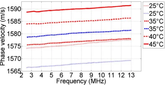
2.5-13.0 MHz. . . 46 3.3 Averaged phase velocity values and standard deviations at 10 MHz

as a function of temperature. . . 47 3.4 Averaged attenuation coefficients in the frequency range of 2.5-13.0

MHz. . . 48 3.5 Averaged attenuation coefficient values and standard deviations at 10

MHz. . . 49 3.6 Comparison between the phase velocity dispersion data and the theo-

retically predicted phase velocity dispersion using the Kramers-Kronig relation. . . 51 4.1 Schematics of the printing techniques employed in the current work. . 58 4.2 Grid of filaments for testing of printing accuracy. . . 62 4.3 Filament target phantom bearing the letters “ITK.” . . . 64 4.4 Ultrasound images of ABS, PLA and DLP phantoms . . . 70

(6)

5.1 PJ phantom trial with different scatterer sizes. . . 77

5.2 Design of PJ SR test phantom. . . 82

5.3 Scattering function of our phantom, the obtained B-mode image and two resulting images of the algorithms using p = 0.5 and 2 norm. . . 84

5.4 Synthetic SF-s and US images of a cat. . . 88

5.5 Synthetic SF-s and US images of a cat with additive noise. . . 88

5.6 SA results validated on a 3D printed phantom. . . 89

5.7 SA test results on a real US image. . . 90

(7)

List of Tables

1.1 Acoustic properties of US phantom manufacturing materials. . . 9

3.1 Fitted linear regression parameters of the phase velocity versus temperature. . . 46

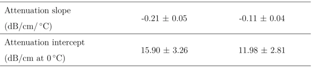
3.2 Fitted linear regression parameters of the attenuation coefficient versus temperature . . . 48

4.1 FDM printing parameters . . . 59

4.2 DLP printing parameters . . . 59

4.3 Acoustic properties of the 3D printing materials. . . 66

4.4 Printing accuracy attained using different printing materials. . . 69

4.5 Resolution parameters of ultrasound images of printed phantoms compared with those of a simulated point scatterer and a true 0.1-mm- diameter nylon filament from a phantom. . . 69

5.1 Modified PJ printing parameters. . . 75

5.2 Axial and transverse FWHM values of a single scatterer from the outer frame of the phantom. . . 85

(8)

Chapter 1 Introduction

Until the end of the previous decade, techniques for manufacturing ultrasound (US) tissue-mimicking materials were limited; also advanced in-house material fabrication techniques were unavailable. Speaking in simple language, as current technology en- ables one to have a device with higher computational power in the pocket than what a PC had some years ago, similarly, near to industrial level material forming technologies are becoming gradually the part of our everyday life, such as the most common 3D printing technologies: namely Fused Deposition Modelling (FDM) or Digital Light Processing (DLP)-based printing. As there are more and more plas- tics becoming available along with countless number of 3D printing techniques, our attention turned to them: Why don’t we try to use them? Possibly there are some materials, which are able to mimick acoustic properties of tissue. However, why is it relevant to mimic human tissues for ultrasound imaging? Or making a step backwards, as the devil’s advocate one can ask: why do we still make research in ultrasound at all? Would not be it more advantageous, to use full-body scans of patients using e.g. computed tomography (CT) or magnetic resonance imaging (MRI), instead of scanning some sector of the body and displaying some (typically) grayscale and strange-looking data to the doctors?

The intention of the author is to clarify these questions in this introduction, providing an easy to follow framework to the reader. The chapter is starting with the motivation behind this dissertation, including the relevance of ultrasound imaging, phantoms and tissue characterization. Also, a brief overview of the dissertation is

(9)

presented. Next, ultrasound phantom manufacturing methods are discussed. Fi- nally, an overview of tissue thermometry, in particular using ultrasound for temperature mapping is presented.

1.1 Motivation

Motivation of current work stems from the questions: is there a way to learn more about ultrasound imaging systems, including the equipment and the efficiency of image enhancement algorithms as well? Is it possible to experimentally recover the transfer function (also called Point Spread Function - PSF) of an imaging system?

The PSF in US is a signal packet, which is scattered back to the transmit/receive unit (usually called transducer) from a tiny inhomogeneity – at the size of the wavelength of the transmitted signal (usually called scatterer) – in an acoustically trans- parent medium (usually called propagation medium). For quantitative measurement of the PSF, it would be important to be able to place scatterers arbitrarily in the propagation medium.

The next step is, if we are able to place such scatterers precisely, is it also possible to fully copy the exact scatterer structure of a medical ultrasound image? And if yes, how to do this? If we could provide solutions for these questions, quantitative measurement of the efficiency of image enhancement algorithms on real ultrasound images would become possible.

1.1.1 Relevance of ultrasound imaging

A sound wave having a frequency over the range of human perception (approximately above 20 kHz) is called ultrasound. In nature, many animals use it for navigation, for example bats or dolphins. Using this recognition the first technological application was developed by Paul Langevin in 1917, where the goal was the detection of submarines. [1]

Nowadays, US has a wide variety of applications such as non-destructive testing, range finding, security systems, low energy data-transfer, welding of plastic parts or biomedical applications. [1–5]

(10)

In medicine US is one of the most widespread medical imaging techniques. In medical imaging the frequency range of 1-20 MHz is usually applied. Since penetration depth and resolution are inversely proportional to each other, lower frequencies are used where higher depths of penetration are required, while higher frequencies will achieve higher resolution at the cost of limited depth of penetration. The main advantage of using US is that it is a non-invasive technique in the classical sense.

Namely, only heating and mechanical effects emerge as a safety issue during examinations. Nevertheless, thermal and mechanical indices are always kept under control and displayed on the screen during operation of the imager. [1]

US is cost-effective compared to MRI and CT, and safe compared to imaging methods using ionizing radiation, while its portability is also a key advantage. In common, US, MRI and CT have their spatial resolution at the same magnitude (usually around a millimeter) [6] and can work in real-time, depending of course on the actually employed algorithm running on a computer.

However, while for example in CT-imaging more complex algorithms are aiming to reduce dosage of ionizing radiation and speed up examinations [7], in ultrasound imaging usually algorithms are aiming to acquire more and more detailed and mean- ingful images while keeping temporal resolution on a reasonable level for real-time imaging [8, 9]. Ultrasound is also useful when fast moving organs like the heart are examined due to its high frame rate [10]. For example combining with Doppler, it is the easiest, cheapest and most safe way to diagnose heart valve disorders [11,12].

In the other hand, due to its portability and scalability it can practically supply a plethora of medical devices and interventions, ranging from monitoring heat deposition during radiofrequency (RF) ablations [13], measuring distances and volumes inside the body, to superficial, high resolution diagnostic devices like DERMUS (http://dermusvision.com).

There are several sources of noise in ultrasound; image quality is often degraded by the presence of speckle artefact, fatty tissues or heated regions can distort and defocus beams as they are acting as acoustic lens [1,6].

(11)

1.1.2 Importance of ultrasound phantoms

In addition to previously mentioned artefacts and noise, it is important to mention that two equivalent subjects of imaging does not exist. This means that using animal models or human volunteers is inadequate to even qualitatively test any properties of an ultrasound imaging equipment [14]. For this reason, ultrasound phantoms are important for checking of image quality and of image resolution enhancement algorithms. Without them current quality of ultrasound imagers and their widespread use would be impossible.

To date, phantom manufacturing methods in ultrasound laboratories are rudi- mentary. Usually phantoms are built up from a propagation medium having acoustic and physical properties similar to average human soft tissue (speed of sound: 1540 m/s [6]; acoustic attenuation: 0.5−1 dB/cm/MHz; density: 1000 kg/m³ [15]). As will be shown in Chapter 3, myocardial tissue shows slightly higher speed of sound values and also different acoustic attenuation. For a specific anthropomorphic phantom that mimics heart, values obtained in Chapter 3 would be more relevant. How- ever, those phantoms are usually designed to include the capability of mimicking blood flow as well as heart movement. The topic of the current thesis is limited to general-tissue stationary phantoms, where the goal is to achieve the above mentioned values for the acoustic parameters.

After an adequate propagation medium was chosen that will be usually doped with sub-wavelength scatterers like microspheres, graphite powder [14] or glass beads [16], which - similarly to real human tissues - introduce speckle into the images. The targets - that reflect strong echoes - are usually made of nylon strings or similar 1D structures comparable in size to the wavelength of the beam (<0.3 mm) [17]. Exact positioning of these strings are possible, however, their number is obviously limited.

Another disadvantage that only the Line Spread Function (LSF) could be extracted instead of the PSF, which is the transfer function of the imaging system. These phantoms are often used for calibration and other quality assurance purposes on imaging equipment [18]. Other type of phantoms are tissue-mimicking phantoms, which can be used for example for training of radiologists or research purposes, e.g.

qualitative testing of algorithms. Here acoustic properties are usually tuned on a

(12)

macroscopic level; the aim is to create a medium similar in shape and size to organs of the human body.

In summary, current phantoms are capable of mimicking a part of human body on a macroscopic scale and are adequate for qualitative and some quantitative tests as well. However, current phantoms lack fully customizable scatterer structure, thus the PSF of a system is unknown (usually modelled using computer simulations) and for this reason, performance of algorithms can be only tested qualitatively.

1.1.3 Importance of tissue characterization

Good quality phantom design relies on accurate characterization of human tissue.

With the widespread adoption of rapid prototyping techniques, a plethora of new materials has appeared for 3D printing. Tissue characterization methods could be also used to characterize these potential tissue-mimicking materials. The most important parameters are the speed of sound and acoustic attenuation, and depending on the exact application, their temperature and frequency dependence as well. The density and the speed of sound determines the characteristic acoustic impedance (Z) of a medium. (For a detailed discussion, see the next chapter.) Based on these properties macroscopic acoustic features of human tissue could be mimicked sufficiently.

Precise characterization is also important for the accurate functioning of advanced ultrasound imaging methods such as ultrasound-based thermometry, which should be sensitive for very small changes (e.g. speed of sound change around 1 m/s).

1.1.4 Overview of current thesis

Here, a brief overview of the following sections and chapters are presented to help the reader.

In the remaining two sections of this chapter, an introduction to medical phantoms and their manufacturing methods, as well as an introduction to tissue thermometry, are given.

(13)

In Chapter 2, the theory of ultrasound imaging is presented, starting with an overview of ultrasound imaging itself. This is followed by sections where physical principles behind the current work are introduced and derived. Finally, characterization of speed of sound and attenuation and the use of Kramers-Kronig relation in ultrasound are discussed.

In the further chapters, the scientific work of the author is presented. In Chapter 3, the temperature and frequency dependence of speed of sound and attenuation in porcine myocardium are presented.

In Chapters 4 and 5, the applicability of 3D printing techniques in US tissue mimicking are shown.

In Chapter 4, two cost-effective, widespread methods (FDM and DLP) are presented as an alternative of currently used calibration phantoms. Here 2D patterns were created, using strings between two supporting walls.

In Chapter 5, an advanced, high resolution 3D printing method (photopolymer jetting - PJ) was used to create arbitrary 3D scatterer distributions. Using such phantoms an image enhancement algorithm was quantitatively tested. Finally, an algorithm is presented, which was developed to create scatterer maps to mimic real ultrasound images. The algorithm allows to tailor properties of the scatterer maps to the printer, like density (spacing) of scatterers.

1.1.5 Declaration of original work used

In this subsection the main references of the current thesis are shown, including the publications of the author, which gives the main basis for the corresponding chapters or sections.

Section 1.2 is based on a part of the Master Thesis of the author [19], which is itself based on [14]. The information used to write Section 1.3 were taken primarily from [20].

In Chapter 2 (Theory of Ultrasound Imaging), Section 2.1 is also partially based on the Master Thesis of the author [19]. In Chapter 2 the further two sections, presenting the derivations of the linear wave equation and scattering are based on [1, 21, 22] and [23], respectively. The discussion of the Kramers-Kronig relation

(14)

(Subsection 2.5.3) is based on [23,24].

The further chapters rest on the scientific work of the author published recently in peer-reviewed journals or in conference proceedings as follows. Chapter 3 is based on [25]. Chapter 4 is based on [26]. In Chapter 5, two conference publications are used as a basis of the text; Section 5.3 relies on [27]. The paper, which provides the basis for Section 5.4 was published at ICU 2017 conference [28].

1.2 Overview of medical phantoms

The aim of this section is to provide the reader a brief summary of the currently used phantoms and phantom manufacturing methods in particular for ultrasound imaging. As mentioned in 1.1.5, the following overview is based on [14].

The idea of phantoms was born in the beginning of the 20th century. After X-ray imaging started to spread and people realized the harmful effects of ionizing radiation the need for tissue substitutes were raised to measure the effects of kilo and megavoltage beams. While in X-ray and CT the most important feature was dosimetry in the first times, quality assurance (QA) became more and more important there and in other imaging modalities (MRI, US, PET) as well. First, very simple phantoms were constructed, e.g. baths filled with water or wax . These were applicable for image uniformity and dosimetry measurements. As materials developed to be more reliable and manufacturing methods evolved as well, reproducibility of more complex phantoms became available, introducing some inhomogeneities inside the imaged volume. Thus, these phantoms could fulfil several QA requirements.

As an example, the most general of these are resolution and contrast measurements, where distinctness of two objects in the region of interest are investigated by the means of spatial distance and signal intensity respectively.

Besides QA, another aim of phantoms is the help of the training of radiologists.

In both cases, a phantom is intend to mimic different physical and radiological properties of human tissue. Movement of organs or the patient (e.g. in CT or MRI) can also be simulated using advanced phantoms.

Exact design of a phantom is specific to its purpose. For example in radiography

(15)

dosimetry phantoms must contain at least one dosimeter placed inside, which in some cases can be moved as well. There are also several types of dosimeters, which could be chosen based on exact design specification of the current phantom. Another example is resolution and image quality measurements, where typically rod or wire targets are placed in a phantom to predefined locations.

1.2.1 Manufacturing of ultrasound phantoms

The first ultrasound phantoms were simple containers with metal rods at specific locations, filled with water providing distance calibration of ultrasound equipment.

The evolution of ultrasound devices demanded better materials with specified and more accurate speed of sound and attenuation that are similar to the properties of living tissue.

These phantoms are useful in ultrasound quality control, and helps better our understanding of the exact physics of ultrasonic wave propagation in tissues that influence imaging performance. Therefore some phantoms are made for experi- mental purposes, for example to measure attenuation, backscatter, and ultrasound exposimetry or bulk material characteristics.

There are three key parameters of ultrasonic phantoms that significantly influence the performance: (1) speed of sound in the phantom, (2) acoustic attenuation (including frequency-dependent attenuation) and (3) scattering (for detailed discussion, see next chapter). There are also other physical parameters like nonlinearity (B/A parameter), but these are not critically important for successful tissue mimicking when applying baseband frequency of the imager. Importance of nonlinear parameters emerges when considering harmonic imaging, however, this is beyond the subject of the current thesis, thus not detailed further. Various methods have been published to prepare “in-house” phantoms made of several materials for teaching and for equipment verifications. The advantage of these phantoms is their low cost and ease of preparation. Nevertheless, the absolute verification of acoustic properties is lacking. [18]

(16)

Material Speed of sound Attenuation Impedance Ref.

[m/s] [dB/cm/MHz] [MRayl]

Agarose-based 1498 − 1600 0.04 − 1.40 1.52 − 1.76 [14]

Avg. Soft Tissue 1540 0.5 − 1 1.5 − 1.7 [6,15]

Gelatin-based 1520 − 1650 0.12 − 1.50 1.60 − 1.73 [14]

Oil Gel-based 1480 − 1580 0.4 − 1.8 1.54 − 1.67 [14]

PAA-based 1540 0.7 @5M Hz 1.7 [14]

Polyurethane 1468 0.13 1.66 [14]

PVA-based 1520 − 1610 0.07 − 0.35 1.60 − 1.77 [14]

PVC-based 1270 − 1580 n.a. n.a. [19,29]

PJ FC 1617 39 @20M Hz 1.87 [30,31]

PJ VW 2633 110 @20M Hz 3.1 [30,31]

Silicone 1030 14.0 @5M Hz 1.1 [32]

Urethane Rubber 1460 0.5 − 0.7 1.31 [14]

Zerdine® 1540 0.5 − 0.7 n.a. [14]

Table 1.1: Acoustic properties of US phantom manufacturing materials. The ab- breviations are as follows: PAA – polyacrylamide; PVC – polyvinylchloride; PJ – photopolymer jetting (3D printing technology), FC – Full Cure, which is a support material for PJ 3D printing; VW – VeroWhite, which is a printing material for PJ 3D printing. Urethane Rubber and Zerdine® are two materials used in commercial phantoms.

Overview of US phantom materials

There are many phantom materials, which are used primarily to prepare “in house”

phantoms or for common use. Some of them are discussed in this paragraph. In the text they are presented qualitatively. A quantitative overview is made in Table 1.1.

Gelatin-based phantoms were widely used as ‘in house’ tools, whose raw material is a homogenous colloid gel derived from collagen – which was extracted from animal tissues – and was one of the earliest attempts to mimic tissues. These can be mixed with alcohol to adjust the speed of sound and graphite powder to adjust scattering.

(17)

The phantom should be stored in benzoic acid in order to avoid bacterial pollution.

The advantage of this material is the relatively good speed of sound and durability at room temperature, when stored in distilled water. It is also cost effective and easy to manufacture. Disadvantages are the temperature sensitivity, the sensitivity against bacteria and the difficulty to achieve uniform scattering.

Another option is the most widely used agarose-gel based techniques. There is also graphite powder used to adjust attenuation and scattering properties. The advantages are the well-characterized performance, the ease and flexibility of the preparation, which allows mixing of several other ingredients to achieve a range of acoustic properties. Recent papers also published on fine-tuning [33] and temperature dependence of acoustic parameters [34] of agarose phantoms. The disadvantages are that agarose phantoms require careful handling, because it is easy to damage, microbial invasion and drying can also occur during storage like in the case of gelatin-based phantoms.

Oil-gel based tissue substitutes containing propylene glycol, a gelatinizer and polymethyl-methacrylate (PMMA) microspheres are also used [14] for phantom manufacture. Their advantages are the immunity to bacterial infection and relatively good physical properties. Unfortunately, since this solution is very rarely used, few information is available about the ease of preparation and applicability.

Polyacrylamide-based phantoms made of acrylamide monomer have speed of sound around 1540 m/s but are highly toxic, and need special precautions.

Polyurethane (PU) phantoms have relatively good physical properties; they are durable and have immunity from bacterial invasion. The disadvantage is that its molecular structure is complex, therefore the standardization is harder, but nowadays 3D printing could give an acceptable solution for standardization. In my previous work [19] PU also investigated using FDM printing, however, with low success factor. The main problem was presumably the air stucked between layers and printed threads.

Polyvinyl-alcohol (PVA) based tissue substitutes have also good physical properties and durability, but the disadvantage here is the emerging difficulties during preparation. It needs several freeze-thaw cycles.

(18)

Silicone was also tested as a material of phantoms because its durability, but it has very low speed of sound and high attenuation, especially in high (above 10MHz) frequencies [14], however, found to be very stable over time and could be suitable for training purposes [32].

Commercially used materials are agarose (preservative technique used, 48 months warranty), Zerdine® (a patented solid elastic material), urethane rubber and thermoplastics. [35]

In our lab, agarose-gel based phantoms are typically used, but the problem is that they are sensitive to physical contact. In addition, due to their high (95−99%) water content, they are liable to drying out, which manifests in damage and extreme size reduction. An alternative could be PVC, which compared to other available materials for “in house” phantom manufacturing has several advantages, for example its chemical resistance and durability. It can be in contact with acids, leaches, oil and petrol, it is also heat resistant in some measure (usually below 80^◦C). More- over it has a low water absorption, which makes it suitable for underwater ultrasonic measurements. Its speed of sound is lower (∼1400 m/s) than propagation speed in average soft tissue (∼1540 m/s), however, it is still considered a proper tissue mimicking material. The main drawbacks are that toxic fumes could be formed during its manufacture and the acoustic properties of the final product largely depends on the exact heat-dose what the material suffered, moreover the storage of the phantom is circumstantial due to the softener base used [19,36]. This softener base gives the majority of these phantoms that also affects longevity of them, as over time leakage of the softener base is observed [19], which affects speed of sound of the propagation medium.

Acoustic characterization of thermoplastics used for 3D printing in ultrasound phantoms were also lacking, however, polyurethane has the same positive properties as PVC that also turned our attention to investigate 3D printing techniques.

Nowadays, 3D printing is mostly used to create mold and vasculature for anthropomorphic US phantoms [37,38], or to create bone-mimicking materials [39–43]. In Chapter 4 applicability of these materials for filament target phantoms are investigated. Recent paper of Jacquet et. al. [30, 31] reported the use of special 3D

(19)

printing photopolymer materials as propagation medium as well. Using a similar technique, the work of the author on the quantitative performance analysis of image restoration methods and manufacturing phantoms with fully customizable scatterer structure are presented in Chapter 5.

1.3 Overview of tissue thermometry

The aim of current section is to provide the reader a brief introduction to tissue thermometry techniques and their relevance both using MR, CT and in particular ultrasound imaging. As mentioned in 1.1.5, the following overview is based on [20]. Nevertheless, the current section is an outlook from the main subject of the dissertation, it is aimed to place the topic of Chapter 3 into context.

There are several procedures in medicine where the intervention involves heating or cooling of tissue. There is a plethora of ablation methods, including radiofrequency-, microwave-, laser-, cryo-, and ferromagnetic ablation, irreversible electroporation and high intensity focused ultrasound (HIFU) as well [44–46].

Tissue thermometry methods are essential, as they make it available to track actual condition of the medical intervention, since the result of the above mentioned treatments are mainly related to the temperature distribution. Using thermal information of the tissue, the medical staff is able to judge which part of tissue remains healthy and which part suffer irreversible changes. Thermal therapies could lead to instant cell death (necrosis), or initiating programmed cell death (apoptosis) – in both cases, the goal is the destruction of undesirable tissue, which is in most of the cases a tumor. Nowadays, minimally invasive – or if available – non-invasive techniques becoming more and more popular, thus for temperature measurements non-invasive techniques are favorable as well [47].

The main aspects choosing between imaging modalities for thermometry are including patient safety, costs, availability, ease of use and compatibility with other devices. Also, the sensitivity, tissue dependence and spatio-temporal resolution are important parameters.

There are three main techniques described below, which are able to acquire data

(20)

deep inside the tissue.

The first one is CT-based techniques. Here the advantages are the compatibility of the imager with other devices, relatively low cost and wide availability of CT machines. However, it is important to note that in this case the patient is exposed to harmful ionizing radiation. The X-ray dose can be reduced with image reconstruction algorithms [7], in turn the result of the temperature measurement could be distorted due to artefacts of image reconstruction [20,46].

MR-based techniques are precise tool of temperature monitoring, although the high cost, the limited availability of these machines and difficulties in compatibility are obstructing their usage. For example, during a surgery all used equipment should be non-magnetic and all of the instrumentation should be resistant for such enormous magnetic fields, which are further increasing the cost of interventions monitored by MRI [46,48,49].

The final group of noninvasive methods are ultrasound-based techniques. US has a relatively low cost, and similar spatial resolution to CT and MR – both performing around some millimeter [20,45,49,50]. However, US thermometry techniques suffer from high tissue-dependence. Nevertheless, US is a safe imaging modality and used many times for guidance of medical equipment inside the body. Once it is used for imaging, it would be also practical to use for thermometry.

1.3.1 Non-ultrasound thermometry

Theoretical background of CT based thermometry

In computed tomography slices of the body are insonified with X-ray radiation.

Data is displayed based on measuring the linear attenuation coefficient of insonified materials. Applying a linear transformation, Hounsfield Units (HU) – or in other words CT numbers – are extracted for each pixel:

CT(x, y) = 1000[µ(x, y))−µH2O]

µ_H₂_O (1.1)

whereµ(x, y) is the average linear attenuation coefficient at pixel position (x, y) and µH2O is the linear attenuation coefficient of water. Temperature measurement

(21)

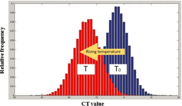
with CT is based on thermal expansion – and hence, density change – of heated tissue. Rate of density change is given by the following equation:

ρ(T) = ρ(T₀)

1 +α∆T (1.2)

where T₀ is the calibration temperature of the CT machine, α is the volumetric expansion coefficient, which is characteristic of the material, and ∆T is the temperature difference between T and T₀.

The change in linear attenuation coefficient can be calculated as:

µ(T) = µmρ(T) (1.3)

where µ_m is the mass attenuation coefficient and ρ(T) is the density of the material at temperatureT.

In summary, the density, and with this, the CT number will decrease as temperature increases as follows:

CT(T) = CT(T₀)− 100µ(T₀)α∆T

µ_H₂_O(T₀) (1.4)

This relation is well illustrated in Figure 1.1, which is adopted from [20].

Theoretical background of MR thermometry

In MR imaging, the resonance frequency of protons is temperature dependent, while the temperature measurements are tissue independent, except fatty tissues. The reason for this difference is while in water the proton resonance frequency is α = 0.01 ppm/^◦C (also called the proton resonance frequency shift coefficient), the proton resonance frequency in lipids are independent from temperature. [50]. The relation between proton resonance frequency phase shift ∆φ and temperature change ∆T is given by the following equation [45]:

∆φ=−∆T ·2π·α·ψ·B₀·T E (1.5) where ψ is the gyromagnetic ratio, B₀ is the magnetic field and T E is the echo time. So, the proton resonance frequency phase shift will be negative if the temperature is rising.

(22)

Figure 1.1: Change of CT value histograms in a water phantom. T₀ corresponds to histogram at calibration temperature and T is the histogram at T₀+ ∆T. Source of figure: [20]

1.3.2 Ultrasound-based thermometry

In ultrasound imaging, thermometry is usually carried out using the knowledge of the speed of sound at ambient temperature inside tissues (generally assumed to be 1540 m/s in soft tissues [13]). Here, similarly to MR imaging, fatty tissues introduce difficulties in temperature monitoring. In normal soft tissues speed of sound is increasing parallel with temperature up to 50-60 ^◦C, and the attenuation coefficient becoming lower simultaneously [51]. This trend turns to the reverse at higher temperatures, moreover, during the cooling back of the previously heated tissue, these values usually does not follow the course which was obtained during heating, due to the irreversible changes in treated tissues. Heat expansion here also plays an important role, as the distance between scatterers becoming bigger.

Active ultrasound

One approach using active ultrasound is temperature monitoring, using channel data delays. As it was mentioned previously, an increase in temperature causes an

(23)

increase in speed of sound of non-fatty tissues. This phenomena will decrease arrival time of the signal where this backscattered beam crosses the heated regions of tissue.

There are examples, where the used tissue model is simple; consist of regions, heated transversely to the imaging plane [13]. To build such models, knowledge of temperature dependence of imaged tissue is essential.

Having the knowledge of temperature dependence of tissue, these simple models can be built and practical to use, when considering a smaller region. In this specific example, monitoring of cardiac radiofrequency ablation was investigated using a transoesophageal (TEE) and an intra-cardiac (ICE) probe. Their aperture are in the range of the extent of heated area, which confirm the choice of the model.

If the aperture is bigger (e.g. a commonly used phased array is employed), there are several techniques, such as speckle tracking, to investigate smaller region of interests. Speckle is usually undesirable, and considered a kind of noise, which makes the images grainy. The phenomenon is arising from sub-wavelength size scatterers.

Thus, in thermometry one can benefit from speckle patterns, as it allows to estimate tissue motion and deformation with high resolution. [50] The estimation of echo- shift is obtained by determining the peak of cross-correlation between consecutive frames (att and t+ 1).

There are some artefacts, which are limiting the accuracy of such temperature monitoring systems. Usually these models are ignoring thermal lensing artefacts and assume tissue heterogeneity. Thermal lensing artefact occurs when the backscattered beam travels through the heated area. As temperature gradients are higher, this distortion is becoming stronger. Using spatial compounding, it is possible to reduce the effect of lensing at the cost of temporal resolution.

As mentioned earlier, the difference between tissues – in particular muscle and fat – can significantly distort the results of such algorithms as they rely on a specific tissue model. In reality both temperature dependence of speed of sound and acoustic attenuation greatly varies from tissue to tissue. The solution is usually to introduce a post-processing algorithm taking into account some known constraints about temperature fields. [50]

(24)

Passive ultrasound

Passive ultrasound thermometry is based on receiving acoustic radiation from the tissues without any acoustic transmission from the imaging transducers. The main difficulty here is that the received signal has very low amplitude compared to active ultrasound methods. Therefore, it usually requires a more complex model, to exclude noise and exclude information outside from the region of interest and acqui- sition takes much more time usually as well. The basic difference is that in active ultrasound one knows the exact time of sound emission, meanwhile in passive ultrasound one has only a receiver unit without the knowledge of the depth of the incoming signal explicitly.

In passive ultrasound, one can measure natural signals radiated by the human body, or in another hand, it can be used to monitor e.g. HIFU treatment. In the first setup, radiation is emitted by chaotic motions inside tissues, which system usually called as an acoustic black body [48, 49]. In the case of HIFU treatment, region of interest (ROI) is irradiated using a high Q number transducer – which means it is emitting long pulses with a very short bandwidth. Thus, cavitation is induced in the ROI. As the focal region is usually a small spatial region (several mm³), the transducer should be moved to destroy all the undesired tissue. For this reason, the time of treatment should be several hours long. During such long treatments, except CT all modalities mentioned in this review are suitable to detect the changes inside, however, it is reasonable to use a method, which does not introduce additional acoustic beam into the ROI. Hence, one convenient way to measure effects of HIFU treatment is using a transducer (-array), which passively detects these changes. The receiver array practically placed transversely to the HIFU beam. [44]

Optoacoustics

Optoacoustics is a phenomena, where a light source irradiates a boundary of the body (this can be the skin, or the intestinal wall using as transrectal probe [47] as well). When the light waves reach such a boundary, some part of it is converted into acoustic energy. During heating or cooling the tissue, the thermoacoustic efficiency (Gr¨uneisen parameter) changes in a linear fashion. Petrova et. al. [47] has

(25)

shown that heat monitoring in highly vascularized tissue can be done, due to the exclusive compartmentalisation of absorbing molecules in hemoglobin. Moreover, this temperature-dependent optoacoustic response was found to be independent of oxygen saturation of blood – so the same response could be obtained from both arterial and venal blood.

1.3.3 Tissue thermometry for cardiac interventions

Nowadays, the most widespread method of cardiac interventions is RF ablation, where different types cardiac arrhythmias are usually cured with high (>95 %) success rate and low morbidity rates [52, 53]. During the intervention current flows through cardiac tissue, heating it due to its electric impedance. It is of major importance to measure temperature in the treated area, to minimize side-effects and complications. Usually, the temperature should not exceed 100 ^◦C to avoid tissue boiling – that means the measured temperature should stay below 70 ^◦C due to temperature measurement uncertainty – which could cause intramyocardial super- heating, ‘pop’ lesions [52] and bleeding of tissue [54]. The standard technique for thermometry is using temperature sensors, usually built in the catheter tip [52]. The main issue with this approach is that the temperature deviation inside the tissue could only be estimated based on the temperature measured on the surface. As it is a living system with great fluid motion, the cooling effect of the blood is also present, which makes this type of temperature monitoring more uncertain. It is also a known issue that RF intervention can cause oesophageal lesion formation and further complications. For this reason, more precise temperature monitoring techniques would be essential. In the literature there are several investigations, where oesophageal lesion formation is intended to be excluded and oesophageal temperature probes were included in the monitoring of the interventions [55,56]. However, M¨uller et. al.

[57] highlights that the use of these probes used for monitoring luminar oesophageal temperature is controversial, as they appears to be a risk factor for the development of oesophageal lesions.

Other approaches are injectable micro-size temperature sensors [58] or IR thermometry, recently presented by Daly et. al. [59]. However, here ultrasound ther-

(26)

mometry could be a nice alternative as it has been also shown by Pasternak et.

al. [13], as a small transducer would be possible to be inserted into the catheter and knowledge of temperature distribution in the axial dimension would be appro- priate to avoid – or at least further decrease the occurrence of – above mentioned complications.

1.3.4 Summary

In summary, the main concept behind image modalities, which are suitable for deep- tissue thermometry, were shown. These are CT, MR and ultrasound. The general advantages and limitations of each were discussed. Each methods can have a spatial resolution around 1mm and provides real-time imaging of the ROI, except some techniques using passive ultrasound where the temporal resolution can be even 1 minute. Finally, an overview of tissue thermometry methods used during cardiac interventions is given, mentioning the opportunities given by ultrasound as well.

(27)

Chapter 2 Theory of Ultrasound Imaging

2.1 Overview of ultrasound imaging

The basic concept of ultrasound imaging consists of three steps: first, a transducer transforms a short, high voltage (∼ns, 100 V) electric signal into a high frequency (∼ MHz) longitudinal pressure wave in a medium; the waves propagate throughout the medium, some of which is scattered or reflected back to the transmitting transducer (or reaches another receiver transducer, depending on the actual setup). Finally, the receiving transducer converts back the pressure changes into an electrical signal, which can then be processed to form an image of the medium properties, such as of the scattering strength distribution in the medium.

The most common type of ultrasound images is the so called B-mode (brightness- mode) image, where the amplitude of the received signal is converted into a grayscale image. The depth that can be seen on these images calculated from the arrival time of the received signal: if the reflector was in a deeper region, the backscattered signal arrives later. To be able to transform time to distance in a trustworthy way, the exact speed of sound of the examined tissue (or other material) must be known or at least well estimated. (Note: the speed of sound in this paper always refers to the propagation velocity of the above-mentioned longitudinal waves in a medium.) For conciseness this introduction will not go into other ultrasound image types, most of them similarly need knowledge of the speed of sound.

One of the basic properties of ultrasound devices is their center frequency that

(28)

highly influence the resolution and penetration depth. These two are inversely proportional, and this gives the most important limitation of ultrasound imaging: if deeper structures are aimed to be imaged, lower frequencies are used and the resolution worsens.

There are two main sources of backscattered energy defined: scattering and reflection. Scattering is usually referred as the interaction of the sound wave with particles smaller than the wavelength, while reflection is such an interaction with particles or objects greater than the wavelength. Both effects are related to the change of density and compressibility of the materials in the way of wave propagation and described by the scattering wave equation (see Section 2.3).

Reflection of waves from the interface of two media is described by the reflection coefficient. The reflection coefficient can be derived from the characteristic acoustic impedances (Z) of the two neighbouring media. Characteristic acoustic impedance (Z) could be derived from the linear wave equation (see Section 2.2), and is specified by the speed of sound (c) and the density (ρ) of a medium:

Z =ρ·c (2.1)

Consider a planar wave travelling from medium 0 to medium 1, having acoustic impedances of Z₀ and Z₁ respectively. The reflection coefficient r describing the proportion (in terms of amplitude) of an incident pressure wave reflected from the interface between two media as follows:

r = Z₁−Z₀

Z₁+Z₀, (2.2)

The above means that in terms of amplitude 1−r part of the incoming wave propagates further into the next medium (acoustic impedance of it is signed as Z₁), the proportion ofr is reflected back to medium 0 (having an acoustic impedance of Z₀). [6]

One important consequence of this relation that ultrasound is best suited to visualize soft tissue, as some structures – for instance bone or airy lungs – are difficult to examine due to the excessively high acoustic impedance contrast with surrounding soft tissue.

(29)

During the development of ultrasound imaging devices or methods, it is often necessary to test the device or method using an object whose properties (mainly speed of sound, attenuation, characteristic acoustic impedance) are similar to tissue, which is, nevertheless, standardized in some way, thus the operator knows what is imaged. When testing for specific image quality metrics of the imaging system, such objects are called calibration or quality assessment (QA) phantoms; these can also be used to assess the degradation of a transducer performance with time. Phan- toms may also be used to model human anatomy and tissue characteristics – called anthropomorphic phantoms – which can be useful for training ultrasound techni- cians in a comfortable environment [18]. This is especially useful when training for uncomfortable and technically demanding procedures such as needle biopsies and rectal examinations.

To manufacture phantoms that fit our purpose, it is first important to know how the physical system works, what is aimed to be mimicked. For this reason, in the next sections the linear wave equation – an idealized but well-working model of pressure wave propagation – is derived first. Thereafter the scattering wave equation is shown briefly, which shows how an inhomogenous system could be modelled.

Based on these, modelling of image formation is presented. Finally, measurement methods of two main phenomena of ultrasound; speed of sound and attenuation are shown complementing the chapter with their linking through the Kramers-Kronig relation.

2.2 Modelling of propagation using linear wave equation

As mentioned in 1.1.5, the following derivation is based on [1,21,22].

In the current thesis only the fundamental frequency of ultrasound imagers are used. Avoiding the use of harmonic imaging allows us to consider the homogenous linear wave equation (LWE) as a good approximation of the underlying physical processes of the examined systems.

However, it is important to note which assumptions and simplifications are made

(30)

to be aware of the limitations of this model. The theory of LWE are best fit for ultrasound pulses travelling in idealized – lossless and homogenous – media. Gen- erally, in soft tissues (but not in hard tissues, such as bone) high frequency shear waves can be neglected due to the high rate of absorption (a factor of 535 for each wavelength travelled [23] p. 87). Due to this simplification, ultrasound wave propagation can be described by a scalar pressure field. However, it should be noted that scalar waves are also affected by attenuation (on the order of 0.5 dB/cm/MHz in tissue, as described in the previous chapter, Section 1.1), which effect in the following derivation is ignored for simplicity. For a discussion of various attenuation phenomena and its effect on wave propagation, please see [6] Chapter 4.

To derive the LWE, the three governing equations of acoustics first need to be derived, namely: I. State equation, II. Continuity equation, III. Force equation.

I. State equation

When a wave propagates through a medium, the local density will change with pressure. This relation is generally superlinear (growing faster than a linear relationship); however, if the changes in density (ρ) and pressure (p) are small compared to the environmental set pointsρ₀, p₀, the relationship can be approximated as linear:

p_total=p₀+p , p << p₀ (2.3)

ρ_total =ρ₀+ρ , ρ << ρ₀ (2.4)

Expecting a linear relationship, the pressure (p) could be expressed as:

p=ερ (2.5)

whereε is a constant and could be expressed from ρ₀ and the compressibility of the mediumκ or its inverse; the elastic modulus K:

ε= 1

κρ₀ = K

ρ₀ (2.6)

(31)

II. Continuity equation

The continuity equation is based on the principle of conservation of mass. Let us suppose we have a cubic control volume V with dimensions dx·dy·dz (see Figure 2.1).

Figure 2.1: Pressure wave acts on a cubic control volume. The pressure change will induce density change of the faces of the cube combined with particle motion. The figure is adopted from [22] .

The mass entering the control volume from face x eqauls:

˙

m_x =ρ_total~u_xdy·dz (2.7)

where ~u denotes ‘particle velocity’; which describes the local motion of small elements of the medium displaced by the pressure. We can use the Taylor series expansion for the mass entering the face atx+dx:

˙

m_x+dx = ˙m_x+ ∂m˙_x

∂x dx+...∼=ρ_total~u_xdydz+∂ρ_total~u_x

∂x dx·dy·dz (2.8)

(32)

Applying this to all directions, the total mass gain per V could be written as:

˙

m_total = ˙m_x−m˙_x+dx+ ˙m_y −m˙_y+dy+ ˙m_z −m˙_z+dz

= −∂ρ_total~u_x

∂x − ∂ρ_total~u_y

∂y − ∂ρ_total~u_z

∂z

!

dx·dy·dz

(2.9)

We know also that the mass gain in V could be written as:

˙

m_total = ˙ρ_totaldxdydz = ˙ρ_totaldV (2.10) Thus, comparing equations 2.9 and 2.10 the following could be written:

˙

ρ_totaldV =−O·ρ_total~u dV (2.11)

From this (original) form of the continuity equation, using Equation 2.4, after simplification and linearisation the final form will be:

−ρ0O·~u= ∂ρ

∂t (2.12)

III. Force equation

For the investigation of the conservation of momentum we use Newton’s law. In the calculations the applied force can be derived from the acceleration~a of particles as follows:

d ~f =dm·~a=dm∂~u

∂t (2.13)

where dm is the mass of the control volume and equals ρ_totaldV.

As can be seen in Figure 2.2, using the pressure, the net force acting in the x direction could be written as:

d ~fx =ptotal(x)dydz−ptotal(x+dx)dy·dz (2.14) Using Taylor series expansion, the force acting onx+dx face could be expanded as:

p_total(x+dx) =p_total(x) + ∂p_total

∂x +... (2.15)

Thus, the net force acting in the xdirection could be rewritten as:

d ~f_x =−∂p_total

∂x dx·dy·dz (2.16)

(33)

Figure 2.2: Force acting in the x direction on the faces of the control volume. The figure is adopted from [22].

Applying Equation 2.16 for all directions, the net force acting on the whole control volume will be:

d ~f =−Op_totaldV (2.17)

Combining Equation 2.13 knowing that dm = ρ_totaldV and Equation 2.17 we get:

ρ_totaldV ∂~u

∂t =−Op_totaldV (2.18)

which can be further simplified, using equations 2.3 and 2.4, to the final form of the force equation:

ρ₀∂~u

∂t =−Op (2.19)

The linear wave equation

To derive the linear wave equation, divergence of the right side of the force equation multiplied by−1 should be taken first. This will give us:

O²p=O·Op=−ρ₀O· ∂~u

∂t = ∂

∂t(−ρ₀O·~u) (2.20) Using the continuity equation (2.12), this could be rewritten as:

∂

∂t(−ρ₀O·~u) = ∂

∂t

∂ρ

∂t = ∂²ρ

∂t² (2.21)

(34)

Combining this with the state equation (Equation 2.5) arranged to ρ=p/εand comparing it with the standard form of the wave equation, we see that ε should equal the square of the speed of sound c². Thus, we will get the final form of the homogenous LWE:

O²p= 1 c²

∂²p

∂t² (2.22)

Derivation of characteristic acoustic impedance

The acoustic impedance is defined as the ratio of pressure to particle velocity, in other words, it represents the resistance of the medium to acoustic wave propagation.

It can be derived from the force equation (Equation 2.19). After rearrangement and integration in time we get:

~

u=^Z −Op

ρ₀ dt (2.23)

In the special case of planar wave propagation, a simple constant specific to the material is obtained, termed the characteristic acoustic impedance, as it is characteristic of the material itself. Without loss of generality, let us suppose the wave propagates in the +x direction, so it can be written as p=A f(x−ct), where f(.) is an arbitrary function describing the shape of the wave. Knowing that the resting state density of the medium ρ₀ is independent of space and time we can get:

~

u=−1 ρ₀

Z ∂Af(x−ct)

∂x dt =− 1 ρ₀

Z

Af⁰(x−ct)dt

=−1 ρ₀ · 1

−cAf(x−ct) = p ρ₀c

(2.24)

So, acoustic impedance Z could be defined as:

Z = p

~

u =ρ₀c (2.25)

where cis the longitudinal propagation speed of sound in the medium.

2.3 Derivation of scattering from the LWE

As mentioned in 1.1.5, the following derivation is based on [23].

Scattering is a phenomenon caused by small inhomogeneities of the medium.

In a physical sense it arises from variations in the compressibility κ and density ρ

(35)

of the medium. Defining the incident field as the field that would arise without such medium variations, the total pressure field p(r, t) (to be precise, this total pressure field does not include the equilibrium pressure, so it is different from p_total in Equation 2.3) can be modelled as the sum of the incident pi(r, t) and scattered p_s(r, t) pressure fields:

p(r, t) = pi(r, t),+ps(r, t) (2.26) In other words, scattering creates virtual sources of the pressure field. To include this into our model, governing equations of acoustics should be expanded as follows.

Equation 2.3 remains the same, however, to take into account the variations in density Equation 2.4 will be:

ρ_total =ρ₀ + ∆ρ+ρ =ρ_υ+ρ (2.27)

and considering the variations of compressibility we get:

κ_υ =κ₀+ ∆κ (2.28)

Thus, the state equation (Equation 2.5) could be modified as:

p= 1

κ_υρ_υρ (2.29)

In the continuity equation the density will change in space, thus it should be rewritten as:

−O·ρ_υ~u= ∂ρ

∂t (2.30)

Similarly, the force equation will be:

ρ_υ∂~u

∂t =−Op (2.31)

Thus, the scattering LWE could be written as:

O· 1 ρ_υOp

!

−κ_υ∂²p

∂t² = 0 (2.32)

Using the above described relationships, the equation could be reformed to ex- press separately the incident and scattered pressure field:

O²p− 1 c²₀

∂²p

∂t² =−O· ∆ρ ρ₀ Op

!

+∆κ κ₀

1 c²₀

∂²p

∂t² (2.33)

(36)

2.4 Modelling of image formation

Image formation in ultrasound is mainly affected by the underlying scattering structure of the imaged medium. Scatterers introduce the well-known grainy noise in the US images, which usually considered as a kind of random noise that degrades image quality; hide parts of the underlying tissue structure in diagnostic imaging, thus adding a subjective judgement of the radiologist to the examination outcome.

Nevertheless, it was found that the speckle artefact on an image is fully deter- ministic. This means that it is caused by the interference of the waves scattered back from the same sub-wavelength particles. Extending the Fraunhofer approximation – introduced originally in optics – ultrasound image formation could be approximated by a linear system. The Fraunhofer approximation states that the far-field complex amplitude pattern created by a complex aperture amplitude function could be approximated by the Fourier transform of that function. [60,61]

Thus, a radiofrequency ultrasound image y could be decomposed to a scatterer map or scattering function x (also known as the tissue reflectivity function [62]) – which includes the Cartesian space coordinates of every scatterer involved in the image – and a point spread function (PSF or h) [60], which is the transfer function of the exact imager:

y=h∗x(+n) (2.34)

where ∗ is the 2D convolution operator and n represents additive random noise (e.g. electrical noise) in the system.

Figure 2.3 illustrates a typical PSF with two types of windowing and the modelling of image formation compared to a real ultrasound image.

(37)

Figure 2.3: Example for the modelling of image formation. On the left side of the image, two simulated PSFs are shown plotted using a 2D rectangular and a Hanning window. To the right there is a typical image of a scattering function can be seen.

On the right side a real B-mode image and a simulated B-mode image are shown.

The simulated image is generated by using Equation 2.34. Figure is adopted from [63]

2.5 Acoustic material characterization

2.5.1 Speed of sound measurement

A variety of speed of sound estimation methods exist, in the literature the two main groups are usually called absolute and relative methods [1]. In absolute methods time of flight (TOF) of the wave is measured without the knowledge of speed of sound of a reference medium. Using absolute methods there are pulsed and continuous wave techniques published.

In relative methods the measurements rely on the knowledge of speed of sound of the reference medium. As a reference medium there are several existing material, which are homogeneous and for which the acoustic properties could be well characterized. These are usually liquids, for example water or saline are usually used for tissue characterization.

In this work relative methods are used for speed of sound measurements, using distilled water as a reference medium. There are two branches of relative methods.

One is the reflection-based method, where the same transducer is used in transmit/receive mode and the backscattered signal is investigated to calculate speed of

(38)

sound values. The other method is the through-transmission measurement, where two transducers are aligned opposite to each other. One of them is the transmitter transducer, which can emit e.g. burst signals at predefined frequencies, the other one is the receiver transducer. Here two measurements are performed in sequence.

First, TOF – and knowing this, speed of sound – in the reference medium is measured, knowing the distance between the surfaces of the transmitter and receiver transducers. Second, TOF in the same path – but with the investigated medium inserted as well – is measured.

Reflection-based measurements

A method, which is similar to that presented below, was used by Dunn et al. [64], however, to fit the measurements to our hardware we used the time-domain instead of frequency domain, although a correct mathematical relationship is lacking in that case. Therefore Equation 2.35 was derived.

For the better understanding, Figure 2.4 illustrates a reflection-based measurement setup. Using Equation 2.35 the unknown speed of sound (v_s) of a sample could be calculated based on the measured TOF values (t_sum – between the transducer and the bottom of the bath, without sample; t_ref – between the transducer and the top of the sample trough reference medium ,t_s– between the two adverse surfaces of the sample) and using the knowledge of the speed of sound in the reference material (v_ref):

v_s =v_ref

tsum−tref

2∗t_s

(2.35)

The time parameters of each measurement can be easily read from an oscil- loscope, however, there are several ways to evaluate speed of sound, depending on where the signal is picked from. In this work the starting point of the wave- package was chosen, however, this is an overestimate of values [1]. Nevertheless, every method has its own source of error. In the equations above v_ref is the speed of sound of the fluid in the bath, which was water in our measurements. This value is temperature dependent and well known in literature [65,66].

(39)

Figure 2.4: The schematic setup for reflection-based speed of sound measurements.

The figure shows the corresponding time, distance and speed of sound values for the reference medium and the sample. s_s is the height of the sample,s_sum is the distance between transducer head and the bottom of the bath. Latter is given by the speed of sound of the water and the TOF without the sample. It is important that during the measurements ssum should be permanent.

Through-transmission measurements

A disadvantage here compared to reflection-based measurements is that the path length of the wave must be known. Measurement error of path length will equal to the measurement error in speed of sound – expressed in percentages (i.e. 0.1 mm error at 10 mm length will introduce 15.4 m/s error in speed of sound when measuring on average soft tissue). This could be fended off using longer path lengths, where the measurement error of path length could be considered negligible. When measuring on thinner samples, a reference medium should be used.

An adequate alignment of the two transducers is crucial. Simple holders for this purpose could be manufactured e.g. using PMMA plates, which have the exact sized holes laser cut into them.