Conference on Modelling Fluid Flow (CMFF’18) The 17th International Conference on Fluid Flow Technologies Budapest, Hungary, September 4-7, 2018
I NVESTIGATION OF TURBOMACHINERY NOISE SOURCES USING BEAMFORMING TECHNOLOGY AND PROPER ORTHOGONAL
DECOMPOSITION METHODS
Bence FENYVESI
1, Eszter SIMON
2,3, Jochen KRIEGSEIS
4, Csaba HORVÁTH
2,51 Corresponding Author. Department of Fluid Mechanics, Faculty of Mechanical Engineering, Budapest University of Technology and Economics. Bertalan Lajos u. 4 – 6, H-1111 Budapest, Hungary. Tel.: +36 1 463-25-46, E-mail: fenyvesi@ara.bme.hu
2 Department of Fluid Mechanics, Faculty of Mechanical Engineering, Budapest University of Technology and Economics.
3 E-mail: eszter.simon24@gmail.com
4 Institute of Fluid Mechanics, Karlsruhe Institute of Technology. E-mail: kriegseis@kit.edu
5 E-mail: horvath@ara.bme.hu
ABSTRACT
This paper presents a combined implementation of phased array microphone beamforming and the Proper Orthogonal Decomposition (POD) methods for the investigation of Counter-Rotating Open Rotor (CROR) turbomachinery noise sources. Acoustic beamforming technology can be applied in order to spatially localise noise sources. When narrowband microphone signal processing is used to create the beamforming maps for each frequency bin, a large dataset can be created. Throughout this dataset, cyclically repeating noise sources will reappear at frequencies associated with the higher harmonics.
Identifying and sorting these noise sources into groups is rather difficult, time consuming, and also subjective. The POD method is widely used for data processing applications as a power-based filtering method, and can therefore be used to filter out the dominant features of the beamforming maps as a function of the frequency. This study presents how the proposed combination of acoustic beamforming and POD can be used in the analysis of turbomachinery applications through the investigation of the shaft order (also known as once- per-rev) noise sources of a CROR test case. Though presented for shaft order noise sources, the presented method is general enough that it can be applied in the identification of other turbomachinery noise sources in future studies.
Keywords: beamforming, shaft order noise source, noise source localisation, phased array microphone, proper orthogonal decomposition NOMENCLATURE
𝑎 [-] weighting coefficient
A [Hz] aft rotor blade passing frequency
B [-] blade number 𝑏𝑓 [-] beamforming vector 𝐵𝐹 [-] beamforming matrix D [-] number of pixels f [-] frequency bin
F [Hz] front rotor blade passing frequency k [-] grid element (pixel)
Ma [-] flow Mach number N [-] number of frequency bins NR [-] filter width
P [-] portion of power PSD [dB/Hz] power spectral density 𝑅 [-] covariance matrix X, Y [-] harmonic indices λ [-] eigenvalue
𝜆 [-] matrix of the eigenvalues μ [-] sectional variance 𝜙 [-] eigenvector
𝛹 [-] matrix of the eigenvectors Subscripts and Superscripts
A aft rotor; all F forward rotor
i frequency bin number j mode number h pixel number
R reduced
S shaft order T transpose
||.|| Euclidean norm 1. INTRODUCTION
With the ever-increasing role of air transportation in our everyday lives, improvements in customer satisfaction and comfort are becoming all the more important. As a result of these demands,
as well as increasingly stringent regulatory practices [1], noise reduction has become a focal point in research related to aircraft engines and turbomachinery applications. To achieve noise reduction goals, noise generation mechanisms first need to be understood. The process starts with the localisation of noise sources, followed by linking them to the phenomena that cause them. Once the noise generation mechanisms are better understood, design changes can be investigated. The results of these investigations will later serve as the basis for design changes.
An effective method of noise source localisation is acoustic beamforming, which relies on measurements carried out with a phased array microphone system. The results are often presented visually in the form of beamforming maps, which depict the dominant noise sources of a given frequency bin. These noise source maps can be simultaneously investigated together with the spectrum created from the peak values of the beamforming maps (referred to as beamforming peaks). Using this combined method of order analysis and noise source localisation, a deeper understanding of the noise generation mechanisms is made possible. In this way, the noise sources can be separated into specific groups, as formerly demonstrated by Horváth et al. [2-4].
While the application of this technique can provide researchers with useful information regarding the noise generation mechanisms of the investigated sources, there are some limitations associated with the method. Since turbomachinery beamforming maps often contain sidelobes [6], as well as rotating coherent noise sources not localised to their true locations [2, 6, 7], their interpretation often requires vast experience and a deeper knowledge regarding the noise generation mechanisms. Carrying out narrowband beamforming investigations also results in a large number of frequency bins, which can make the analysis of a set of data rather confusing and time consuming.
Aiming to reduce the involvement of the aforementioned subjective elements, in this paper, the combined implementation of beamforming and the Proper Orthogonal Decomposition (POD) method is investigated for turbomachinery noise sources. The POD method (also known as Karhunen- Loève expansion and principal component analysis) has been successfully applied in numerous scientific disciplines, meteorology [8], molecular biology [9]
and the pattern recognition of various physical and medical phenomena, especially for the analysis of complicated velocity fields [10-11]. The POD algorithm provides an orthogonal basis for representing a given data set, and finds an optimal, lower dimensional approximation. Hence it can be used to reduce the degrees of freedom of a complex system, and accomplish the reconstruction of the
dataset without losing significant details and components of the inspected phenomena.
The present study examines the combined application of the two methods through the investigation of the shaft order noise sources of a Counter-Rotating Open Rotor (CROR) aircraft engine. Shaft orders, otherwise known as once-per- rev noise sources, are associated with occurrences which repeat once every revolution, or multiples thereof. In this particular case, a piece of measurement instrumentation was found to be mounted on one of the blades of the aft rotor. If one were to examine the aeroacoustic noise associated with this instrumentation in a rotating reference frame, it would have a broadband character.
Investigated in a stationary reference frame, the noise heard can be described as broadband, having an envelope curve which oscillates at the same frequency as the once-per-rev [4]. The noise generation mechanisms investigated herein are therefore associated with the rotational speeds of the rotors, which plays a key role in the way in which the method applied in this study has been defined. It is also known, that since these are rotating broadband noise sources that appear cyclically (appearing as tonal peaks in the spectrum), that they will be localised to their true noise source positions by beamforming [4].
As a first step in investigating the shaft order noise sources, the beamforming maps for a chosen CROR measurement test case have been created using a beamforming process appropriate for the given test configuration. In our case, delay-and-sum beamforming in the frequency domain has been applied, carrying out a custom narrowband processing of the data in order to help highlight the tonal peaks in the spectra, while not limiting the spatial extent of the noise sources on the beamforming maps due to the application of deconvolution methods. From the Beamforming Peak (BFpeak) values of each frequency bin, a Power Spectral Density (PSD) spectrum has been created, and by simultaneously applying order analysis and investigating the beamforming maps, noise sources can be sorted into categories. This process requires considerable knowledge regarding the turbomachinery noise sources under investigation, is time consuming, and is somewhat subjective. The process is considered somewhat subjective, because many of the noise sources are localised to the same general area, often overlapping, and therefore, it is hard to decide which noise source group to associate a given noise source with. Therefore, in order to help eliminate the subjectivity associated with separating apart the noise sources, and to make the process simpler and faster, the beamforming maps are processed with various POD approaches. By applying the POD method, features of the beamforming dataset (which in this case are examined as a function of frequency) can be
extracted, and hence a further analysis, grouping, and even filtering of the noise generation mechanisms is made possible. To identify and subsequently quantify the influence of shaft order noise sources, the groups of noise sources are processed with separate PODs. Particular emphasis is then placed on the POD post-processing in the common base sense [11] to quantify the impact of the shaft-order noise. This novel approach advances the state of the art available in the literature by providing a less subjective, less difficult, and somewhat automatable means for separating apart the various noise sources seen in a series of beamforming maps into subgroups.
2. MEASUREMENT SETUP
Measurements were carried out on the Open Rotor Propulsion Rig (ORPR) in the NASA Glenn Research Centre 9×15 ft Low-Speed Wind Tunnel (LSWT) [2, 3]. The setup is shown in the bottom of Figure 1. The F31/A31 historical baseline blade set was used during the tests [12]. The open rotor configuration is roughly 1/7th scale, the forward blade row consists of 12 blades with a diameter of 0.652 m, while the aft rotor has 10 blades with a diameter of 0.630 m. Further details regarding the ORPR and the blade set can be found in [12].
The test configuration which is to be investigated herein is that of an uninstalled CROR (not having a pylon), being examined at the take-off nominal condition, with a blade angle of 40.1° on the forward rotor, and a blade angle of 40.8° on the aft rotor. The angle of attack with regard to the wind tunnel flow of Ma 0.2 was 0°. The corrected standard day value of the rotational speed was set to 6450 RPM for both rotors. These tests were a part of a larger test campaign of aerodynamic as well as aeroacoustic investigations. Further details regarding the test set-up and the test matrix can be found in [2, 3, 12].
Acoustic measurements were carried out using the OptiNAV Array48 phased array microphone system [12]. The array consists of 48 flush-mounted Earthworks M30 microphones fixed in a 1m x 1m aluminium plate (see top of Figure 1.). A camera is also built into the centre of the plate, which is used to take a photo of the field of view of the phased array system. This image is loaded into the data processing software, in order to make it possible to superimpose the noise source localisation contour maps on the photo.
The microphone signals were simultaneously recorded at a sampling rate of 96 kHz and then processed using the delay-and-sum beamforming method in the frequency domain [5]. In order to improve the signal-to-noise ratio of the results, a long sampling time of 45 s, as well as the removal of the diagonal of the cross-spectral matrix were applied.
The array was installed in a cavity of the sidewall of the wind tunnel, at a distance of 1.6 m from the centre
plane of the test rig. A Kevlar® sheet was tightly stretched over the opening of the cavity, in order to provide a smooth aerodynamic surface for the flow, while also allowing acoustic waves to pass through.
The Kevlar® sheet, together with the measurement setup, can be seen in the bottom part of Figure 1.
Figure 1. The Array48 microphone system and its installation in the wall of the LSWT [4]
3. PROCESSING OF THE RESULTS As discussed above, one way of evaluating the results of turbomachinery noise measurements is to examine the dominant noise sources of a given frequency bin by investigating the largest noise sources located on the beamforming maps together with the BFpeak PSD spectrum. This combined method is useful for sorting noise sources, but is rather difficult, time consuming, and somewhat subjective. On top of it, the method does not provide us with any further information regarding noise sources which are reoccurring throughout the frequency domain. The dataset is processed using order analysis. An emphasis is placed on relevant CROR noise sources, which are to be sorted into three main categories. For better presentation and comparison of the data sets to the results of other CROR and turbomachinery noise investigations, the bandwidths of the frequency bins used herein do not
agree with conventional bandwidths, but are determined by dividing the frequency range between two harmonics of the Blade Passing Frequency (BPF) of the aft rotor into 50 equal bins.
The first group of the investigated noise sources is that of rotating coherent noise sources, which are associated with interaction tones and blade passing frequencies. The interaction tones are comprised of the harmonics of the BPF of each rotor written in the form XF+YA, X and Y being positive whole numbers, while the BPF of the Forward and the Aft rotors are referred to as F and A respectively.
A somewhat larger category is that of rotating incoherent noise sources, which can be further divided into two main subgroups. When the dominant noise sources on the beamforming maps are located on the surface of a rotating element, and are localised to the same position for a wide frequency range, they are sorted into the subgroup of broadband noise sources.
Investigating the data set after the removal of the rotating coherent noise sources, it can be found that there are some remaining peaks in the PSD spectrum.
These peaks fall into the category of shaft orders, commonly referred to as once-per-rev tones, which are the second subgroup of rotating incoherent noise sources. Since the generation mechanism of this noise source can be associated with blade-to-blade inconsistencies of a given blade row, if the observer were to move together with the blades, noise sources in this category would be considered as broadband noise sources. However, they appear as tonal peaks rising out of the broadband. This is due to the fact that they are associated with once-per-rev frequencies, and hence, from the viewpoint of the phased array, they appear at the same location once for every revolution. As a result, these sources are having an envelope curve which oscillates with the rotational frequency of the rotor. It has been found, that shaft order tones of this particular test case are localised to a noise source appearing on the pressure side of the aft rotor near the blade tip, which is a direct result of a measurement instrumentation mounted on one of the blades.
A typical example for beamforming results of a shaft order noise source can be seen in Figure 2. The top of the figure shows the beamforming map of the given frequency bin. The dynamic range is limited to 5 dB with respect to the beamforming peak value.
The bottom of the figure presents the PSD spectrum of the BFpeak.
After creating the beamforming maps and the beamforming peak spectrum of the data set, the sorting procedure was carried out, separating the CROR noise sources into the aforementioned categories. The spectrum of the test case was therefore decomposed into three main components, as shown in Figure 3. Rotating coherent noise sources are marked with continuous black lines.
These are the most dominant peaks of the spectrum.
It can also be observed, that noise sources in the frequency bins of the BPF are of smaller amplitudes, and are usually associated with shaft orders (dashed red lines) or rotating broadband noise sources (grey line), since the amplitudes of rotating coherent noise sources, especially BPF tones, drop off very quickly with increasing frequency.
Figure 2. Beamforming results for a shaft order noise source
Figure 3. Groups of various CROR noise sources While investigating turbomachinery noise sources via the sorting method presented above provides useful information regarding the noise generation mechanisms of CROR, as well as the distribution and amplitudes of the various noise sources along the investigated frequency range, there are some difficulties associated with the method.
One limitation is a consequence of the involvement of subjective visual inspection in the process. As
mentioned before, as a result of the presence of multiple noise sources in the same frequency bin, interpretation and analysis of beamforming maps and the PSD spectrum requires experience and specific prior knowledge. Hence, due to the complexity of the investigation and the noise generation phenomena, a degree of uncertainty is incorporated in the investigation, which also affects the repeatability of the method. Moreover, since the use of the narrowband beamforming process results in a large number of frequency bins for the investigated frequency range (725 for this particular test case), the complete analysis of data sets can be overwhelming.
This work aims to propose a method for processing the beamforming maps, and localising turbomachinery noise source groups, while overcoming some of the aforementioned difficulties.
The main goal is to lessen the subjectivity of the investigations, which leads to the introduction of the POD analysis.
4. POD ANALYSIS
Generally, principal component analysis, such as the POD for instance, determines the characteristic degrees of freedom as contained in the underlying basis, which are usually referred to as principal components or the modes of the given problem.
Frequently, only the most energetic part of such an orthonormal basis is considered to serve either as a basis for reduced-order-model (ROM) efforts or simply to filter the data in the correlation space [10].
If the raw data basis furthermore is comprised of various subgroups of information, then a Common- Base POD (CPOD) of the data allows quantitative comparison between these groups [11].
As the POD method centers around an Eigenvalue problem, it in turn decreases the use of subjective judgement during the process, such as visual inspection. A further advantage of POD is that information about the relative energy contribution of the components to the overall noise can be immediately connected to spatial noise patterns in the time and/or frequency domain.
4.1. Implementation of the POD method To perform the proper orthogonal decomposition, beamforming maps of each 𝑓𝑖 (i=1:
N) frequency bin are to be described as 𝑏𝑓𝑖 beamforming vectors. The elements of the vectors are the beamforming values of their respective noise source maps, each value pertaining to a 𝑘(𝑗)(j=1: D) element (pixel) of the grid of the inspected acoustic field. A 𝑏𝑓𝑖 vector can be constructed by putting the pixel-columns of their beamforming maps after one- another, the first element being the top left pixel of the source map (see Eq. (1)). A visual explanation about the indices of 𝑏𝑓𝑖 is given in Figure 4 for the reader’s convenience.
𝑏𝑓𝑖= [
𝑏𝑓(𝑘(1), 𝑓𝑖) 𝑏𝑓(𝑘(2), 𝑓𝑖)
⋮ 𝑏𝑓(𝑘(𝐷), 𝑓𝑖)]
(1)
Collecting the beamforming vectors over the N frequency bins, the 𝐵𝐹 beamforming matrix is to be given as
𝐵𝐹 = [𝑏𝑓1 𝑏𝑓2… 𝑏𝑓𝑁]. (2)
Figure 4. Visual explanation of the indices of the beamforming vector
The 𝑅 covariance matrix is built according to Eq.
(3), hence, the corresponding eigenvalue problem can be written according to Eq. (4).
𝑅 = 𝐵𝐹 𝐵𝐹𝑇. (3)
𝑅 𝛹 = 𝜆 𝛹. (4)
Then, the 𝜆 matrix of the λj (j=1: N) eigenvalues
𝜆 = [ 𝜆1
0 𝜆2
⋱ 0
𝜆𝑁
] (5)
and the 𝛹 matrix of the 𝜙𝑗 eigenvectors 𝛹 = [𝜙1 𝜙2 … 𝜙𝑁] (6) can be determined, which is referred to as the POD basis. As outlined above, the eigenvectors also represent the modes of the POD algorithm. Using the λj eigenvalues, the energy contribution of each mode to the overall power is
𝑃𝑗= 𝜆𝑗
‖𝜆‖. (7)
Using the 𝛹 matrix of the 𝜙𝑗 eigenvectors, the 𝑎𝑖 weighting coefficients can be calculated as
𝑎𝑖= 𝛹 𝑏𝑓𝑖. (8) The source maps in this new basis can be reconstructed as a superposition of the product between the weighting coefficients and the POD modes according to
𝑏𝑓𝑖= ∑𝑁𝑗=1𝑎𝑗𝑖 𝜙𝑗= 𝛹𝑇𝑎𝑖. (9) Note that any reduced number of modes in Eq.
(9) leads to the aforementioned filtering and/or ROM approach. Furthermore, it is important to mention that the variance of any mode’s coefficient across the N source maps is identically equal to the corresponding eigenvalue by definition, i.e.
1
𝑁∑𝑁𝑖=1(𝑎𝑗𝑖)2= 𝜇𝑗𝑁≝ 𝜆𝑗. (10)
4.2. POD analysis of the data set
When applying POD in Matlab® [13]
environment to investigate the shaft order noise sources of the existing CROR test case, three different subsets have been examined. The first subset is the same as the original data set, as all of the frequency bins are included. This set will be referred to as ALL with 𝑁 ∶= 𝑁𝐴 source maps. As mentioned in Chapter 3, shaft order noise sources are associated with once-per-rev frequencies. Therefore, the centre frequencies of the frequency bins, in which they are expected to appear, can be determined by dividing the BPF of the rotor on which they are located (A), with the blade number of the rotor (BA) (see Eq. (11)).
𝑓𝑠ℎ𝑎𝑓𝑡 𝑜𝑟𝑑𝑒𝑟 = 𝑓𝑅𝑃𝑀= 𝐴/𝐵𝐴 (11) Since these noise sources, appear in a repetitive pattern along the whole frequency range (even when they are not the most dominant noise sources of their respective frequency bins), their inclusion in the POD analysis can be altered effortlessly. Thus, the second subset is comprised of the beamforming maps of every frequency bin which should contain a shaft order noise source (referred to as SHAFT ORDER), while the third subset is comprised of the maps of every frequency bin which does not contain a shaft order noise source (referred to as REVERSED).
These two subsets are comprised of the accordingly reduced numbers of source maps 𝑁𝑆 and 𝑁𝑅, respectively, where 𝑁𝑆+ 𝑁𝑅= 𝑁𝐴 leads back to the full number of considered maps.
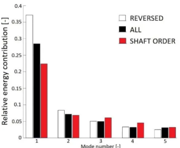
The eigenvalues of the first five POD modes are shown in Figure 5. A significant difference between the relative energy contributions of the first modes between the considered subsets can be identified.
However, since the separate eigenvalue problems reveal different principal components, i.e. noise patterns, no direct (quantitative) comparison across the PODs is possible beyond the identification of trends. Here, the REVERSED group seems to dominate the first two modes, where the SHAFT ORDER subsets only come into play from the third modes.
Figure 5. Relative energy contribution of the first five modes for various PODs.
The different energy contributions of the modes are immediately connected to the corresponding modal noise pattern, hence the various noise generation mechanisms can be identified. When investigating the POD maps of the first five modes, it can be observed, that the patterns seen on the maps are to some extent similar for the all the subsets of each mode. In addition to the varying magnitudes also slight differences of the patterns can be identified for the different subsets.
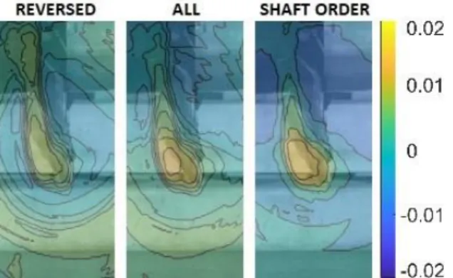
Figure 6. POD maps of Mode 3
One such example is given in Figure 6 for Mode 3, where – at least at first glance – the ALL subset seems to be the superposition of the REVERSED and SHAFT ORDER subsets. The measurement setup is also given in the background for clarity. It can be seen, that the dominant noise sources are localised to the blade of the aft rotor where the measurement instrumentation was mounted, hence to the location of shaft order tones (see the surrounding of the source enlarged in Figure 7.).
Figure 7. Mode 3 – The close surrounding of the measurement instrumentation mounted on a blade of the aft rotor
However, based on these observations, it is hypothesized that the majority of the energy contribution of the shaft order sources falls into the third and fourth POD modes. This hypothesis is tested below by means of the CPOD approach.
4.3. CPOD analysis of the data set Given that the 𝑁 source maps should be rated on a quantitative level, it becomes important to advance beyond the separate analysis of the 𝑁𝑆 and 𝑁𝑅 maps in separate PODs. Initially the CPOD was proposed to quantify the impact of parameter variations to given field information under investigation [11]. In the present context, the CPOD-based post processing is utilized to identify and quantify the different noise source patterns within one particular experiment.
Particularly, the impact of the shaft order subset is to be quantified. Accordingly, the eigenvalue problem of the full basis 𝑁 = 𝑁𝐴 is considered to ensure identical modes across the investigated subsets. The contribution of either subset to the modes is then derived from the sectional variances
1
𝑁𝑆∑𝑁𝑠=1𝑆 (𝑎𝑗𝑆)2= 𝜇𝑗𝑁𝑆 and (12a) 1
𝑁𝑅∑𝑁𝑅=1𝑅 (𝑎𝑗𝑅)2= 𝜇𝑗𝑁𝑅. (12b) where the indices of 𝑎𝑗 (S and R) are maps from the SHAFT ORDER (𝑁𝑆) and REVERSED (𝑁𝑅) subsets, respectively. The sum of sectional variances, by definition, adds up to the eigenvalue of the respective modes, i.e.
𝜇𝑗𝑁𝑆+ 𝜇𝑗𝑁𝑅= 𝜇𝑗𝑁≝ 𝜆𝑗, (13) which is indicated by the stacked contributions in Figure 8. The meaning of Eq. (13) can be immediately identified from direct comparison of Figures 8 and 5 (black bars). In order to identify whether a noise pattern occurs predominantly due to
shaft order noises, the ratio 𝜇𝑗𝑁𝑆/𝜇𝑗𝑁𝑅 is shown in Figure 9.
Figure 8. Relative energy contribution of the first five modes for the CPOD approach colour coded according to the noise source.
Figure 9. Energy ratio between shaft order and other noise sources for the first five modes.
Since shaft order noise is expected in every fifth bin, a ratio of 0.25 indicates an evenly distributed contribution. Therefore, values above or below 0.25 indicate whether the respective patterns are shaft- order dominated or, respectively, not.
Figure 9 saliently demonstrates that the above hypothesis regarding the impact of shaft order noise sources hold for Mode 3, but was disproved for Mode 4. Furthermore, the quantitative rating of Figure 9 uncovered Mode 5 to be a major contributor for shaft order tones.
5. SUMMARY
The present investigation has introduced an approach for investigating turbomachinery noise sources using a microphone array, by combining the advantages of beamforming technology with those of order analysis and POD (modal) analysis. The study first introduced a method of investigation, in which, the various noise sources of the examined CROR setup have been sorted into groups considering their noise generation mechanisms. While providing useful information, it was concluded, that there are some limitations associated with this process, due to the involvement of subjective visual inspection.
Hence, as an alternative approach, the proper
orthogonal decomposition was introduced in the investigations, and the shaft order noise sources of the CROR test case were further analysed. First, POD was used to determine the relative energy contribution of the POD modes of different subsets of the original data. Here, it was identified that the comparison between different PODs uncovers formerly hidden trends, but is inappropriate for quantification. A more rigorous analysis was, therefore, performed by means of a CPOD approach, where the impact of either subset was evaluated from the entire data set. Particularly, it was found for the present setup that the majority of the shaft order noise sources can be found in the third POD mode. It has also been concluded that CPOD analysis is an effective method to identify and localise noise sources with different energy contributions without a time consuming sorting process and special prior knowledge. While overcoming many of the difficulties of previously applied methods, subjective elements are still involved during the interpretation of the POD results. Since there are multiple noise generation mechanisms present in every frequency bin, the development of an advanced pre-processing method is to be considered, in order to filter the audio signal before the creation of the beamforming maps.
ACKNOWLEDGEMENTS
The testing of the CROR was funded by the Environmentally Responsible Aviation Project of the NASA Integrated Systems Research Program and the Fixed Wing Project of the NASA Fundamental Aeronautics Program. The present investigation was supported by the Hungarian National Research, Development and Innovation Center under contract No. K 119943, the János Bolyai Research Scholarship of the Hungarian Academy of Sciences, the Higher Education Excellence Program of the Ministry of Human Capacities in the frame of the Water science & Disaster Prevention research area of the Budapest University of Technology and Economics (BME FIKP-VÍZ), as well as the TeMa Talent Management Foundation.
REFERENCES
[1] Peake, N., Parry, A. B., 2012, “Modern Challenges Facing Turbomachinery Aeroacoustics”, Annual Review of Fluid Mechanics, Vol. 44(1), pp. 227-248.
[2] Horváth, Cs., Envia, E., Podboy, G. G., 2014,
„Limitations of Phased Array Beamforming in Open Rotor Noise Source Imaging”, AIAA Journal, Vol. 52(8), pp. 1810-1817.
[3] Horváth, Cs., 2015, “Beamforming Investigation of Dominant Counter-Rotating Open Rotor Tonal and Broadband Noise Sources”, AIAA Journal, Vol. 53(6), pp. 1602- 1611.
[4] Fenyvesi, B., Tokaji, K., Horváth, Cs., 2018,
“Investigation of a pylons effect on the character of counter-rotating open rotor noise using beamforming technology”, Acta Acoustica united with Acoustica. (Under Review)
[5] Dougherty, R. P., 2002, “Beamforming in acoustic testing”, in: Mueller, T. J., (Ed.), Aeroacoustic Measurements, Springer-Verlag, Berlin, pp. 62-97.
[6] Parry, A. B., Crighton, D. G., 1989, “Prediction of Counter-Rotation Propeller Noise”, AIAA 12th Aeroacoustics Conference, San Antonio, TX, USA, paper no. AIAA-89-1141.
[7] Hanson, D. B., 1984, “Noise of counter-rotation propellers”, AIAA 9th Aeroacoustics Conference, Williamsburg, VA, USA, paper no.
AIAA-84-2305.
[8] Preisendorfer, R. W., 1988, “Principal Component Analysis in Metereology and Oceanography”, Elsevier, Amsterdam
[9] Stein., S. A. M., Loccisano, A. E., Firestine, S.
M., Evanseck, J. D., 2006, “Principal Components Analysis: A Review of its Application on Molecular Dynamics”, Elsevier, Amsterdam
[10] Meyer, K., Pedersen, J., Özcan, O., 2007, “A turbulent jet in crossflow analysed with proper orthogonal decomposition”, Journal of Fluid Mechanics, Vol. 583, pp. 199-227.
[11] Kriegseis, J., Dehler, T., Gnirß, M., Tropea, C., 2010, “Common-base proper orthogonal decomposition as a means of quantitative data comparsion”, Measurement Science and Technology, Vol. 21(8), pp. 957-233.
[12] Van Zante, D. E., Gazzaniga, J. A., Elliott, D.
M., Woodward, R. P., 2011, “An Open Rotor Test Case: F31/A31 Historical Baseline Blade Set”, 20th International Symposium on Airbreathing Engines, Gothenburg, Sweden, paper no. ISABE 2011-131
[13] MATLAB® Commercial Software, The Math Works Inc., www.mathworks.com
![Figure 1. The Array48 microphone system and its installation in the wall of the LSWT [4]](https://thumb-eu.123doks.com/thumbv2/9dokorg/1394640.116239/3.892.473.787.229.741/figure-array-microphone-installation-wall-lswt.webp)