Investigation of Rotating Coherent BPF Noise Sources via the Application of Beamforming and Proper Orthogonal
Decomposition
Fenyvesi, Bence1
Budapest University of Technology and Economics (BME), Faculty of Mechanical Engineering, Department of Fluid Mechanics
1111 Budapest, Bertalan Lajos utca 4-6, Hungary
Kriegseis, Jochen2
Karlsruhe Institute of Technology (KIT), Institute of Fluid Mechanics 76131 Karlsruhe, Kaiserstraße 10, bldg. 10.23, Germany
Horváth, Csaba3
Budapest University of Technology and Economics (BME), Faculty of Mechanical Engineering, Department of Fluid Mechanics
1111 Budapest, Bertalan Lajos utca 4-6, Hungary
ABSTRACT
Rotating coherent noise sources are major contributors to the noise of various turbomachinery applications having contra-rotating blade sets. The noise sources are associated with Blade Passing Frequencies (BPF) and interaction tones, which are comprised of the harmonics of the BPFs. The present study examines BPF noise sources through the combined application of two distinct methods in the investigation of the noise of a Counter-Rotating Open Rotor (CROR) aircraft engine. In a first step, in order to localize the noise sources of CROR, acoustic beamforming is performed on a data set of phased array microphone measurements.
Then, Proper Orthogonal Decomposition (POD) is used to filter out the dominant features of the beamforming maps as a function of the frequency. Particular emphasis is placed on the POD post-processing in the common-base sense to quantify the impact of the BPF noise. It is found that the POD-based post processing can be utilized to make a connection between the relative energy contributions of BPF turbomachinery noise sources to their spatial noise patterns, furthermore, their impact to the overall noise can be quantified and visualized.
Keywords: Noise source localization, Beamforming, Proper orthogonal decomposition, Rotating coherent noise source, Phased array microphone
I-INCE Classification of Subject Number: 70 _______________________________
1 fenyvesi@ara.bme.hu
2 kriegseis@kit.edu
3 horvath@ara.bme.hu
NOMENCLATURE
𝑎 weighting coefficient B blade number
BPF blade passing frequency 𝑏 beamforming vector
𝐶 CPOD map
f frequency
Ma flow Mach number
N number of frequency bins and modes M reduced number of frequency bins P portion of power
𝑄 beamforming matrix 𝑅 covariance matrix λ eigenvalue
𝜆 matrix of the eigenvalues μ variance
𝜙 eigenvector
𝛹 matrix of the eigenvectors Subscripts and Superscripts
A aft rotor F forward rotor
i frequency bin (map) number j mode number
R reversed 1. INTRODUCTION
Often the most bothersome noise generated by fans and various turbomachinery applications is that occurring at the Blade Passing Frequencies (BPF). This sound not only occurs at high sound pressure levels, but usually tends to be the most dominant noise source in the most sensitive frequency region of human hearing. The blade passing frequency noise of a propeller or fan is comprised of thickness and loading noises [1, 2].
As machines with rotating blade sets (fans, aircraft propellers, etc.) are designed to produce a pressure difference, the potential flow fields of their blades will create lobes of circumferential spinning modes, which will travel toward the observer at the speed of sound [3]. Since the pressure fluctuations of these coherent wavefronts are associated with the blade number – hence with the blades passing frequency – they will produce noise at the harmonics of the BPF. It is also known, that if the blade row of another rotor or stator is very close to a rotor, a potential flow field interaction can exist between them [4, 5]. Therefore, another type of rotating coherent noise source, which can be significant, is the interaction between rotor and stator, or – in the case of counter-rotating configurations – the interaction between two rotors. These will be referred to as interaction tones. A viscous type interaction can also be associated with blade passing frequencies, which occurs when the rotor blade wakes strike the blades of the rotor (or the stator) downstream to it. The components of this generation mechanism are usually referred to as blade-wake interaction tones [5]. The present study aims to investigate the
blade passing frequency noise related to the rotating coherent structures of the first category, which are referred to as the blade passing frequency tones throughout the text.
While BPF noise sources appear as tonal peaks in the spectrum, the relative strengths of their discrete (or narrow band) frequencies and the broadband components will vary with the type of turbomachinery application considered [6]. For instance, the noise of low tip speed fans is almost entirely broadband, while the noise from many high speed aircraft engines is mainly characterized by discrete frequency tones [6]. In this report, a combined investigation method is presented for the examination of the BPF noise sources of a Counter-Rotating Open Rotor (CROR) aircraft engine. As these complex aeroacoustic configurations produce a wide range of tonal and broadband noise, the generation and contribution of blade passing frequency noise needs to be explored to determine the possibilities of reducing noise at the source.
Acoustic beamforming together with phased array microphone measurement technology is used herein in order to localize and visualize dominant noise sources for the pre-defined frequency bins of the investigated frequency range. Then these spatial noise patterns (referred to as the beamforming maps) can be examined together with the power spectral density spectrum created from the beamforming peak values of the individual maps. As it was formerly demonstrated by Horváth et al. [3, 5, 7], a more complex understanding of noise generation mechanisms is made possible via the application of this joint method, and noise sources can also be separated into specific groups. However, there are limitations associated with this method [3, 8], since many of the noise sources are often localized to the same general area, which can at times create overlaps, thus their interpretation usually relies on visual inspection. Consequently, their categorization can at times be rather subjective and non-quantitative, whilst requiring vast experience and a deep knowledge of the investigated generation mechanisms.
Furthermore, narrowband beamforming investigations also result in a considerable number of frequency bins, hence the thorough analysis of a set of data is often complicated and time consuming.
This study presents the implementation of the combined method of beamforming and Proper Orthogonal Decomposition (POD) to the investigation of rotating coherent BPF noise sources. The general methodology was first introduced to the acoustic community by Fenyvesi et al. in [9]. The main goal with the method is to lessen subjectivity and increase repeatability while creating the possibility of high-level automation. It proposes an alternative means to effectively describe complex, high- dimensional beamforming data sets in a low-dimensional form, via the application of modal decomposition. First, the beamforming maps and the spectrum have been created from the phased array microphone measurement data set of the chosen test case using an appropriate beamforming process [5, 9]. Then, instead of the manual separation and sorting of the CROR noise sources into categories which was applied in the past [3, 5, 7, 9], the data set of the beamforming maps (which in this case is examined as a function of frequency) were used as input for the POD analysis. The fact, that the noise generation of the BPFs are associated with the rotational speeds of the rotors plays a key role in the way in which the applied method has been defined. As a result, the important features can be extracted, while further analysis and grouping of the generation mechanisms is made possible. By applying the proper orthogonal decomposition in the Common-based sense (CPOD) [10], additional information can be gained in the process, since the method also helps to better identify and subsequently quantify the impact of BPF noise sources. This information then can be used to create new spatial noise patterns in order to visually demonstrate the relative energy contributions of the investigated frequency bins of the blade passing frequencies to the resulting POD modes.
2. MEASUREMENT SETUP
The measurements were carried out at the NASA Glenn Research Center on the open rotor propulsion rig of a 9×15 ft low-speed wind tunnel [3, 7]. A CROR configuration of 1/7th scale was used during the tests, equipped with the F31/A31 historical baseline blade set [11]. The forward blade row has 12 blades with a diameter of 0.652 m, the aft rotor – being slightly smaller – consists of 10 blades with a diameter of 0.630 m. Figure 1 shows a schematic drawing of the equipment including the basic metrics, as well as the directions of rotation for the rotors. As seen from the upstream direction, the forward rotor rotates in the clockwise direction, and the aft rotor rotates in the counter-clockwise direction.
The test configuration which is to be investigated herein is that of a standalone counter-rotating open rotor, examined at the take-off nominal condition. This flight-stage for the given configuration is characterized by a blade angle of 40.1° on the forward rotor, and a blade angle of 40.8° on the aft rotor. The angle of attack with regard to the wind tunnel flow of Ma 0.2 was set to 0°. The corrected standard day value of the rotational speed was set to 6450 RPM for both of the rotors, resulting in blade tip Mach numbers roughly around 0.62. Further details regarding the test set-up, the blade set and the test matrix of the measurement campaign can be found in [3, 7, 11].
Figure 1 – Sketch of the measurement setup of the CROR engine: a) side view, as seen from the viewpoint of the array; b) top view
Figure 2 – a) The phased array microphone system; b) the installation of the array in the wall of the wind tunnel together with the open rotor test rig [3]
The experimental setup is shown on the right hand side of Figure 2. Aeroacoustic measurements were carried out using a phased array microphone system (OptiNAV Array48, see [12]), which consists of 48 flush-mounted Earthworks M30 microphones installed in a 1m x 1m aluminum plate. A camera is built into the center of the plate, which is then used to take a photo of the field of view of the array. Being loaded into the
data processing software, this image makes it possible to superimpose the noise source localization contour maps on the photo of the investigated setup. The phased array was installed in a cavity of the sidewall of the wind tunnel, at a distance of 1.6 m from the center plane of the test rig (see Figures 1 and 2), which can be considered to be in the acoustic far-field according to simulations carried out by Horváth et al. [3, 7]. A Kevlar®
sheet was tightly stretched over the opening of the wall cavity, in order to provide a smooth aerodynamic surface for the flow, while also allowing acoustic waves to pass through. Microphone signals were simultaneously recorded at a sampling rate of 96 kHz and then processed. In order to improve the signal-to-noise ratio of the results, a sampling time of 45 s was applied.
3. PROCESSING OF THE RESULTS
As a first step of the investigation, beamforming has been carried out, and noise source maps have been created from the phased array microphone measurement data set of the chosen CROR test case. In our case, delay-and-sum beamforming in the frequency domain [8] has been performed with custom narrowband data processing. The frequency range between each BPF of the aft rotor (BPFA) was divided into 50 equal bins. The investigated frequency range starts at the first blade passing frequency of the aft rotor and ends at the 15th, thus it contains 700 bins, each having widths of 19.1 Hz. The center frequencies of the frequency bins in which the BPFs are expected to appear can be determined using the rotational speed (RPM) of the rotor which they are associated with (forward or aft), and the blade number of the rotor (B) according to Equations 1a and 1b.
It can be seen, that the fundamental blade passing frequencies of the configuration are therefore in the most sensitive frequency region of human hearing [13], as the value of BPFF is 1290 Hz, while the BPFA is 1075 Hz.
𝑓𝐵𝑃𝐹𝐹 = RPM
60 ∙ 𝐵𝐹 = 𝑓𝑅𝑃𝑀∙ 𝐵𝐹 (1a) ; 𝑓𝐵𝑃𝐹𝐴 =RPM
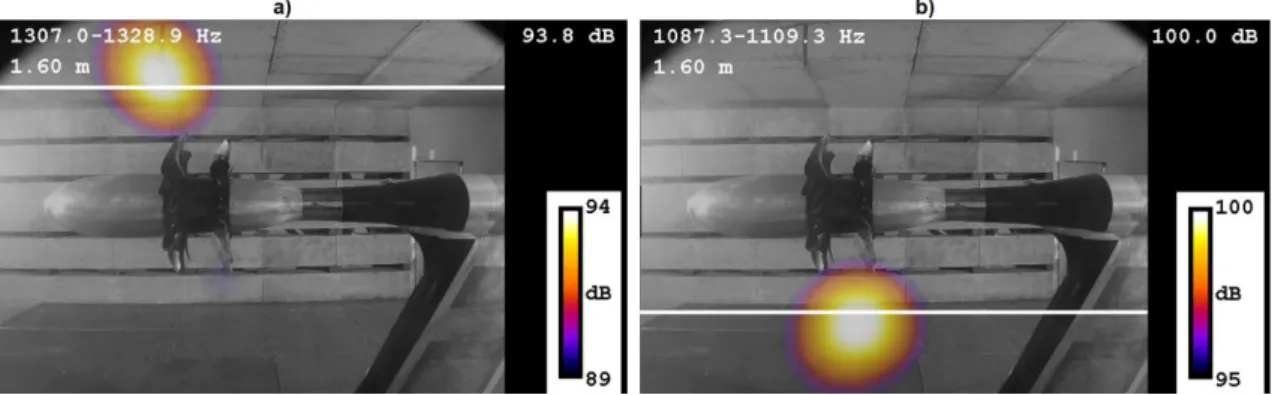
60 ∙ 𝐵𝐴 = 𝑓𝑅𝑃𝑀∙ 𝐵𝐴 (1b) It was established in former studies, that standard beamforming processes trace the wavefronts of rotating coherent noise sources back to apparent noise source locations, which do not agree with the true noise source locations, even if those locations are not on the blades [3]. These sources rather align with their Mach radii, which refer to the radial position at which the lobes of circumferential spinning modes travel toward the observer at the speed of sound. For the rotating coherent noise sources of BPF tones, the values of the Mach radii will always be positive [3], hence apparent noise sources will be localized to the side of the axis where the rotor is spinning toward the observer. For subsequent harmonics of the blade passing frequencies, the calculated values of the Mach radii point to the same radial positions, hence similar noise sources related to the harmonics of the BPFs are expected.
The apparent noise sources of BPF tones will be localized only to the rotors they are associated with. As a consequence of the fact, that the rotors are spinning in the opposite direction (see Figure 1), the Mach radius of BPFF will be located above, while the Mach radius of BPFA will be located below the horizontal axis of the CROR setup on the beamforming maps.
Figure 3 depicts rotating coherent noise sources, pertaining to the fundamental (first) BPFs of the forward and aft rotors respectively, which are localized to their Mach radii, marked with white lines. Information pertaining to the frequency ranges under investigation are given in the top left corners. Since turbomachinery beamforming maps often contain undesirable sidelobes [14], in our case, the beamforming maps are plotted using a 5 dB dynamic range with respect to the maximum values of the maps, which are
referred to as the beamforming peaks (given in the top right corners). Therefore, the displayed beamforming values on each of the maps show the most dominant noise sources of their investigated frequency bins.
Figure 3 – Beamforming results for rotating coherent noise sources: a) BPFF; b) BPFA
In many instances, the dominant noise source associated with a given frequency bin is more than 5 dB higher than the other less significant noise sources in the same bin.
Therefore, most of the less significant noise sources will fall below the plotted dynamic range in this investigation, including many of the apparent noise sources associated with BPFs, since the amplitudes of BPF noise sources drop off quickly with increasing frequency. Consequently, BPF noise sources at high frequencies are usually not the most dominant sources of their frequency bins, which presents difficulties when investigating turbomachinery noise sources via a manual sorting method [5]. Furthermore, this sorting method can be rather subjective at times, and since the use of the narrowband beamforming process results in a large number of frequency bins for the investigated frequency range, the complete analysis of data sets can be overwhelming. Addressing the aforementioned issues, it can be stated, that more advanced, automatic means of investigation are necessary, which leads to the introduction of POD analysis.
3.1 Implementation of POD
Proper orthogonal decomposition (also known as principal component analysis) has been successfully applied in numerous scientific disciplines, especially for pattern recognitions of various phenomena, such as the investigation of complex velocity fields [10, 15]. Principal component analysis, determines the characteristic degrees of freedom as contained in the underlying basis of a data set, which are usually referred to as principal components or modes of the given problem. Doing so, it aims to find an optimal, lower- dimensional approximation via seeking for an orthogonal basis to describe a particular data set [15, 16]. Then often only the most energetic part of the orthonormal basis is considered to serve as a basis for a reduced-order-model. As the POD method mainly centers around an eigenvalue problem, it decreases the use of subjective judgement during the process, such as visual inspection, while increasing the possibility of high-level automation.
Even though the inputs of POD are usually snapshots of scalar or vector fields in the time domain, it is now performed in the frequency domain in order to determine the principle components of the data set of the beamforming maps. As an input for the POD algorithm, the beamforming maps of the N frequency bins are described as vectors, which are referred to as the beamforming vectors (𝑏𝑖 ; i = 1 : N). Elements of the vectors are the beamforming values of their respective noise source maps, each value pertaining to an element of the grid of the inspected acoustic field. After the creation of the beamforming vectors, they are collected over the range of the N frequency bins into a beamforming
matrix (𝑄), as shown in Equation 2. The objective of the POD analysis is to find the optimal basis vectors that can best represent the given data, i.e. we seek a set of vectors that can represent 𝑄 in an optimal manner, hence with the least number of modes. First, the 𝑅 covariance matrix is constructed according to Equation 3, and then the solution to the problem can be determined by finding the 𝜙𝑗 (j = 1 : N) eigenvectors and the 𝜆j eigenvalues of the corresponding eigenvalue problem (Equation 4).
𝑄 = [𝑏1 𝑏2… 𝑏𝑁] (2)
𝑅 = 𝑄 𝑄𝑇 (3)
𝑅 𝛹 = 𝜆 𝛹 (4)
The size of the covariance matrix is related to the spatial degrees of freedom of the data, and hence it is equal to the number of grid points. The 𝛹 matrix of the 𝜙𝑗 eigenvectors found from Equation 4 is called the set of the POD modes. They are a set of orthogonal modes, and their respective eigenvalues convey how well each eigenvector captures the original data. Then the eigenvalues are collected in the 𝜆 eigenvalue matrix, in which they are arranged in decreasing order, and therefore the modes of the POD are arranged in order of importance with respect to their representation of the energy of the acoustic field. The matrices are shown in Equations 5 and 6. As shown in Equation 7, the 𝑃𝑗 energy contribution of each mode to the overall power can be determined by dividing the 𝜆𝑗 eigenvalues by the Euclidean norm of the eigenvalue matrix.
𝜆 = [ 𝜆1
0 𝜆2
⋱ 0
𝜆𝑁
] (5)
𝛹 = [𝜙1 𝜙2 … 𝜙𝑁] (6)
𝑃𝑗 = 𝜆𝑗
‖𝜆‖ (7)
From the 𝛹 matrix of the 𝜙𝑗 eigenvectors, the weighting coefficients of the POD modes (𝑎𝑖) can be calculated (Equation 8). Then the fluctuations in the original field are to be expressed as a linear combination of the modes and their corresponding weighting coefficients (Equation 9). In other words, the source maps in this new basis can be reconstructed as a superposition of the product between the weighting coefficients and the POD modes.
𝑎𝑖 = 𝛹 𝑏𝑖 (8)
𝑏𝑖 = ∑𝑁𝑗=1𝑎𝑗𝑖𝜙𝑗 = 𝛹𝑇𝑎𝑖 (9)
Furthermore, as shown in Equation 10, the variance of any mode’s coefficient across the N beamforming maps can be calculated from the corresponding eigenvalue by dividing it with the total number of the maps.
𝜇𝑗𝑁= 1
𝑁∑𝑁𝑖=1(𝑎𝑗𝑖)2 ≝𝜆𝑗
𝑁 (10)
It is important to mention, that currently the degree of freedom of this new basis is equal to that of the original data set of beamforming maps (N = N). As the eigenvalues are arranged in decreasing order, the modes of the POD are arranged in the order of importance in terms of capturing the energy of the acoustic field. The eigenvalues then can be used to determine the number of modes needed to represent the original data in an optimal (lower-dimensional) manner.
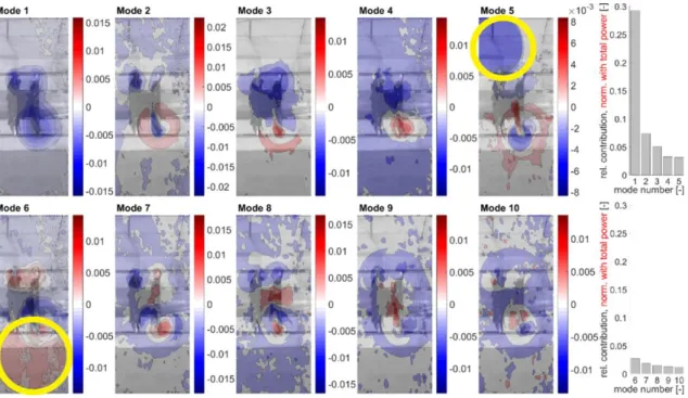
Figure 4 – POD maps and relative energy contributions for the first ten modes The POD maps of the first ten modes together with their relative energy contributions are shown in Figure 4. The different energy contributions of the modes are related to the corresponding modal noise patterns, hence the various noise generation mechanisms can be identified. It can be seen, that the majority of the energy contribution is found into the first five POD modes. Based on the comparison of the modal noise patterns to the spatial noise patterns of the BPFs presented in Figure 3, it can be seen – at least at first glance – that the majority of the energy contribution connected to the noise sources of BPFF falls into mode 5, while BPFA noise sources seem to dominate mode 6.
These patterns are highlighted in the top right, as well as the bottom left corner on the POD maps above using yellow circles. The hypothesis is tested below by means of the CPOD approach.
3.2 Implementation of CPOD
If the basis of the raw data is comprised of various subgroups (groups of noise sources for instance), then a common-base proper orthogonal decomposition (CPOD) of the initial data set allows for a quantitative comparison between the subgroups [10]. A further advantage of CPOD is that information regarding the relative energy contributions
of the components to the overall noise can be determined and immediately associated with the noise patterns. In the present context, the CPOD-based post processing is utilized in order to identify and quantify the impact of subsets pertaining to the BPFs. Since these noise sources appear in a well-defined repetitive pattern along the whole frequency range, their inclusion in the POD analysis can be altered almost effortlessly.
For the investigation of the effect of the BPFnoise sources of the forward rotor, the first subset is comprised of the beamforming maps of every frequency bin which should contain a BPFF noise source (even when they are not the most dominant noise sources of their respective frequency bins). The second subset is comprised of the maps of every frequency bin which does not contain a BPFF source. These two subsets are comprised of the accordingly reduced numbers of source maps 𝑁𝐹 and 𝑁𝐹𝑅, respectively, where F denotes the BPFs of the Forward rotor, while FR refers to Forward Reversed.
𝑁𝐹+ 𝑁𝐹𝑅 = 𝑁 leads back to the full number of the considered maps. A similar naming system is used during the quantification of the impact of the BPF noise of the aft rotor.
The contribution of the subsets to the modes is then derived from the sectional variances according to Equations 11a, 11b, 12a and 12b, where indices of 𝑎𝑗 (F, FR, A and AR) are maps from the given subsets, respectively.
1
𝑁𝐹∑𝑁𝐹=1𝐹 (𝑎𝑗𝐹)2 = 𝜇𝑗𝑁𝐹 (11a) ; 1
𝑁𝐹𝑅∑𝑁𝐹𝑅=1𝐹𝑅 (𝑎𝑗𝐹𝑅)2 = 𝜇𝑗𝑁𝐹𝑅 (11b)
1
𝑁𝐴∑𝑁𝐴=1𝐴 (𝑎𝑗𝐴)2 = 𝜇𝑗𝑁𝐴 (12a) ; 1
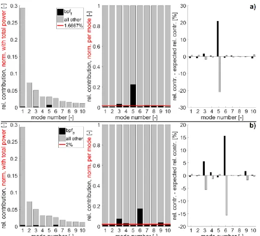
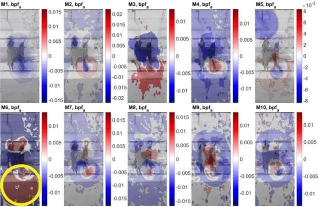
𝑁𝐴𝑅∑𝑁𝐴𝑅=1𝐴𝑅 (𝑎𝑗𝐴𝑅)2 = 𝜇𝑗𝑁𝐴𝑅 (12b) In accordance with Equation 10, the sums of sectional variances, add up to the eigenvalues of the respective modes divided by the N number of the beamforming maps (see Equation 13), which is indicated by the stacked contributions in Figure 5. In order to identify whether a noise pattern occurs predominantly due to BPF noise sources, the energy ratios 𝜇𝑗𝑁𝐹/𝜇𝑗𝑁𝐹𝑅, as well as 𝜇𝑗𝑁𝐴/𝜇𝑗𝑁𝐴𝑅 can be defined and compared to the values of the expected evenly distributed contributions (𝑁𝐹/𝑁𝐹𝑅 and 𝑁𝐴/𝑁𝐴𝑅). Therefore, energy ratio values above or below this limit (marked with a red line in Figure 5) indicate whether the respective patterns are BPF dominated or not. Furthermore, the energy ratios can also be used to visualize the relative impacts of the subsets on the modal noise patterns (see Equations 14a and 14b). These weighted modal noise patterns will be referred to as the CPOD maps (𝐶𝑗).
𝜇𝑗𝑁𝐹+ 𝜇𝑗𝑁𝐹𝑅 = 𝜇𝑗𝑁𝐴+ 𝜇𝑗𝑁𝐴𝑅 = 𝜇𝑗𝑁 ≝𝜆𝑗
𝑁, (13)
𝐶𝑗𝐹 =𝜇𝑗
𝑁𝐹 𝜇𝑗𝑁
𝑁
𝑁𝐹𝛹𝑗 (14a) ; 𝐶𝑗𝐴 = 𝜇𝑗
𝑁𝐴 𝜇𝑗𝑁
𝑁
𝑁𝐴𝛹𝑗 (14b)
The CPOD maps of the first ten modes are shown in Figures 6 and 7. Based on the examination of the weighted modal noise patterns and the relative energy contributions, it is found that mode 5 is dominated by BPFF noise sources, while the frequency bins of BPFA dominate for modes 3 and 6. However, due to the presence of multiple noise generation mechanisms in each of the frequency bins, the relative dominance of the blade passing frequency noise of the aft rotor is not as conspicuous for mode 3, as the corresponding modal noise pattern does not only resemble to the usual shape and location of the concentrated noise pattern associated with BPFA, but also shows
similarities to that of shaft order noise sources [5, 9]. It can be stated, that the investigated BPF noise sources are not the most dominant for the given CROR test case, since the majority of their energy contributions can be found in less energetic modes.
Figure 5 – Relative energy contributions of the first ten modes color coded according to their subsets: a) BPFF; b) BPFA
Figure 6 – Weighted CPOD maps for the first ten modes: BPFF
Figure 7 – Weighted CPOD maps for the first ten modes: BPFA
4. CONCLUSIONS
Turbomachinery noise sources pertaining to the blade passing frequencies of a counter-rotating open rotor were investigated using the combined implementation of beamforming and proper orthogonal decomposition methods. It can be stated, that the automatic, objective and far less time-consuming separation of BPF noise sources via the application of modal decomposition was successful. POD was effectively used to determine the relative energy contributions of the different subsets of the original data to the modes, then the impacts of the subsets to the corresponding modal noise patterns were also visualized by the means of CPOD. The process yields results that are easy to comprehend without special prior knowledge, which is an important advancement as compared to the formerly used manual sorting process. Particularly, it was found for the present setup, that the BPF noise sources can be found in less energetic modes. For conclusion, it can be stated, that the method applied herein can be used for the analysis of turbomachinery noise sources of various kinds. The next step is to develop a method for the reconstruction of the data set where only the part of the orthonormal basis is considered for which the investigated (BPF) noise sources are dominant. Then the resulting new data set would only contain the noise sources which are relevant to the current investigation. Furthermore, the effect of different dynamic range settings should also be looked at, and the development of an advanced pre-processing method could also be considered in order to further improve the quality of the results.
5. ACKNOWLEDGEMENTS
This paper has been supported by the Hungarian National Research, Development and Innovation Centre under contracts No. K 119943, and the János Bolyai Research Scholarship of the Hungarian Academy of Sciences, and by the ÚNKP-18-4 New National Excellence Program of the Ministry of Human Capacities. The research reported in this paper was supported by the Higher Education Excellence Program of the Ministry of Human Capacities in the frame of Water science & Disaster Prevention research area
of Budapest University of Technology and Economics (BME FIKP-VÍZ). The authors gratefully acknowledge financial support from DAAD Eastern Partnership (2019-2021), as well as the support of the TeMa Talent Management Foundation.
6. REFERENCES
1. J. S. Jang, H. T. Kim, W. H. Joo, “Numerical Study on Non-Cavitating Noise of Marine Propeller”, Inter-noise 2014, Melbourne, Australia 2018.
2. T. F. Brooks, D. S. Pope, M. A. Marcolini, “Airfoil self-noise and prediction”, NASA Technical report, Report no. NASA-RP-1218, 1989.
3. Cs. Horváth, E. Envia, G. G. Podboy, „Limitations of Phased Array Beamforming in Open Rotor Noise Source Imaging”, AIAA Journal, Vol. 52(8), 2014, pp. 1810-1817.
4. J. H. Dittmar, “Methods for reducing blade passing frequency noise generated by rotor-wake - stator interaction”, NASA Technical report, Report no. NASA TM X-2669, 1972.
5. B. Fenyvesi, K. Tokaji, Cs. Horváth, “Investigation of a pylons effect on the character of counter-rotating open rotor noise using beamforming technology”, Acta Acustica united with Acustica, Vol. 105(1), 2019, pp. 56-65.
6. I. J. Sharland, “Sources of noise in axial flow fans”, Journal of Sound and Vibration, Vol. 1(3), 1964, pp. 302-322.
7. Cs. Horváth, “Beamforming Investigation of Dominant Counter-Rotating Open Rotor Tonal and Broadband Noise Sources”, AIAA Journal, Vol. 53(6), 2015, pp. 1602-1611.
8. R. P. Dougherty, “Beamforming in acoustic testing”, in: Mueller, T. J., (Ed.), Aeroacoustic Measurements, Springer-Verlag, Berlin, 2002, pp. 62-97.
9. B. Fenyvesi, E. Simon, J. Kriegseis, Cs. Horváth, “Investigation of turbomachinery noise sources using beamforming technology and proper orthogonal decomposition methods”, 17th International Conference on Fluid Flow Technologies (CMFF’18), Budapest, Hungary, paper no. CMFF-32, 2018.
10. J. Kriegseis, T. Dehler, M. Gnirß, C. Tropea, “Common-base proper orthogonal decomposition as a means of quantitative data comparsion”, Measurement Science and Technology, Vol. 21(8), 2010, pp. 957-233.
11. D. E. Van Zante, J. A. Gazzaniga, D. M. Elliott, R. P. Woodward, “An Open Rotor Test Case: F31/A31 Historical Baseline Blade Set”, 20th International Symposium on Airbreathing Engines, Gothenburg, Sweden, paper no. ISABE 2011-131, 2011.
12. Optinav Inc., Array 48, http://www.optinav.info/Array48.pdf, 2017.
13. D. B. Robinson, “The subjective loudness scale”, Acta Acustica united with Acustica, Vol. 7(4), 1957, pp. 217-233.
14. A. B. Parry, D. G. Crighton, “Prediction of Counter-Rotation Propeller Noise”, AIAA 12th Aeroacoustics Conference, San Antonio, TX, USA, paper no. AIAA-89-1141, 1989.
15. G. Berkooz, P. Holmes, J. L. Lumley, “The Proper Orthogonal Decomposition in the Analysis of Turbulent Flows”, Annual Review of Fluid Mechanics, Vol. 25(1), 1993, pp.
539-575.
16. K. Taira, S. L. Brunton, S. T. M. Dawson, C. W. Rowley, T. Colonius, B. J. McKeon, O. T. Schmidt, S. Gordeyev, V. Theofilis, L. S. Ukeiley, “Modal Analysis of Fluid Flows:
An Overview”, AIAA Journal, Vol. 55(12), 2017, pp. 4013-4041.
![Figure 2 – a) The phased array microphone system; b) the installation of the array in the wall of the wind tunnel together with the open rotor test rig [3]](https://thumb-eu.123doks.com/thumbv2/9dokorg/1076007.72200/4.892.160.736.746.970/figure-phased-array-microphone-installation-array-tunnel-rotor.webp)