1
TOWARDS A DOPPLER EFFECT BASED BEAMFORMING METHOD FOR ROTATING COHERENT NOISE SOURCES
Csaba Horváth and Bálint Kocsis
Budapest University of Technology and Economics, Faculty of Mechanical Engineering, Department of Fluid Mechanics
Bertalan Lajos utca 4-6, 1111 Budapest, Hungary
ABSTRACT
The beamforming literature proposes a selection of methods for the investigation of rotating noise sources. These methods are very useful, each having its own advantages and disadvantages, but none of them have been developed with the goal of localizing rotating coherent noise sources. This investigation collects the advantages of each method and proposes outlines for two methods designed specifically for rotating coherent noise sources. Both methods are based on the Doppler Effect, which helps separate the microphone signals of the individual rotating coherent noise sources from one another, making it possible to trace them back to their true noise source locations rather than their Mach radii.
1 INTRODUCTION
Turbomachinery technology is continuously advancing, as competitors develop new products, striving to be the best in a given segment of the market. Noise level is one turbomachinery design aspect, which has received increased attention from consumers over the years. Societal expectations regarding a quiet work and living environment are reflected not only in product sales, but also in new legislations, which limit noise levels, and hence the products which are allowed to appear on the market. Turbomachinery noise consists of multiple components, which can be categorized in many different ways. From a beamforming perspective, one important aspect which needs to be kept in mind is the coherence of the noise sources. Many typical turbomachinery noise sources are rotating coherent noise sources, and as a result of this property, currently available beamforming methods often have difficulty in accurately localizing them to their true noise source positions on the individual blades and distributing the source strength appropriately. This investigation looks at the properties of rotating coherent noise sources and proposes an alternative approach for localizing them to their true noise source locations.
2
To date, multiple beamforming methods have been developed which are customized for the investigation of rotating noise sources, including the Rotating Source Identifier (ROSI) method of Sitjsma, Oerlemans, and Holthusen [1], the beamforming for rotative sources method of Minck, Binder, Cherrier, Lamotte, and Budinger [2], the rotating beamforming method of Pannert and Maier [3], and the rotating sound source method of Herold and Sarradj [4]. All four of these methods are similar in that they have been developed with the intent of investigating rotating noise sources. The method proposed herein differs in that it approaches the problem with the specific goal of localizing rotating coherent noise sources, or in other words rotating noise sources which can be characterized by a time invariant phase relationship. The four methods stated above differ in many ways, each having its own advantages and disadvantages. The method of Sijtsma et al. [1] was the first of these methods to be developed. It is carried out in the time domain, where the signals measured on the microphones are delayed and summed after the Doppler shift and the distance between the investigated source position and the microphone is corrected for. The method of Minck et al.
[2] is also carried out in the time domain. Time domain based methods have the disadvantage of being time consuming, and also being incompatible with other high-resolution frequency domain based source characterization beamforming methods, which utilize the Cross-Spectral Matrix (CSM). The frequency domain based beamforming methods of Pannert et al. [3] and Herold et al. [4], on the other hand, take advantage of the CSM provided opportunities.
Though this makes them robust with regard to the applicability of high-resolution beamforming methods, these methods are more restrictive in the way in which measurements need to be carried out. Both frequency domain based methods utilize phased arrays which are circular, axially centered, and have microphones placed at tangentially evenly spaced positions in a given ring.
Most currently available beamforming methods determine the frequency content of the investigated microphone signals using the Discrete Fourier Transform (DFT) [5]. The disadvantage of using such a method in order to decompose a signal into its frequency components is that it is characterized by a low temporal resolution. Recent investigations have looked at applying other methods of decomposing the signal during the beamforming process, such as the Discrete Wavelet Transform (DWT) [6] and Short-Time Fourier Transform (STFT) [7]. Though other investigations might have applied these transformations for reasons other than improving the temporal resolution, this property should be kept in mind in developing beamforming methods for moving sources.
Turbomachinery noise sources are often categorized into two main groups, tonal and broadband noise sources. Tonal noise sources are characterized by a discrete frequency, and in the case of turbomachinery are often associated with the regular cyclic motion of the rotor blades with respect to a stationary observer and with the interaction of the rotors with adjacent structures [8]. These are referred to as Blade Passing Frequency (BPF) tones and interaction tones, respectively. Broadband noise sources are characterized by a wide frequency range, and are associated with the turbulent flow in the inlet stream, boundary layer, and wake [8]. While broadband noise sources are most often not coherent, many tonal turbomachinery noise sources often are.
As discussed above, this investigation attempts to provide a solution for localizing rotating coherent noise sources using beamforming technology. The method introduced herein is based on the advantages and disadvantages of the existing methods discussed in [1-4], taking into account what is known about the Mach radius effect and the Doppler Effect. The following sections will first describe rotating coherent noise sources and what happens when
3
we apply beamforming to them, then the significance of the Doppler Effect in localizing rotating coherent noise sources will be looked at, followed by a detailed investigation of the method of Sijtsma et al. [1], and finally an approach will be proposed for localizing rotating coherent noise sources.
2 ROTATING COHERENT NOISE SOURCES
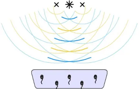
The coherence of noise sources is important in beamforming, since coherent noise sources most often give misleading beamforming results. As wave fronts propagate away from coherent noise sources, they interact constructively and destructively, and the interaction patterns of the wave fronts make it hard to accurately localize the true noise source positions using most beamforming methods. This is visualized in Fig. 1 for the generic case of stationary coherent monopole noise sources, marked in the figure by 𝑥. As the wave fronts propagate away from the sources, they interact to form a wave front of higher amplitude (darker lines), which appears to radiate from an apparent noise source location positioned between the noise sources. The signal is recorded by a phased array of microphones (located at the bottom of the figure), and when processing the data using most beamforming methods, a strong noise source will appear at the apparent noise source position to where the normal of the wave front of large amplitude can be traced back to using beamforming technology. This apparent noise source position is marked in the figure by ∗.
Fig. 1. Two stationary coherent noise sources investigated with a phased array of microphones. The wave fronts interact constructively and destructively to form a wave front of large amplitude, which appears to be radiating from the point marked by ∗ in the figure.
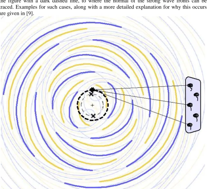
The interaction patterns of rotating coherent noise sources also give misleading results when investigated in a stationary reference frame, as the apparent source positions to which the noise sources are localized by beamforming in the stationary reference frame do not point to the actual noise source positions, but rather point to their Mach radii [9]. The name “Mach radius” or “sonic radius” refers to the mode phase speed, the speed at which the azimuthal lobes of a given azimuthal mode rotate around the axis, having a Mach number of 1 at the Mach radius (𝑧∗, a normalized radius, where 𝑧∗ = 1 refers to the blade tip) when examined from the viewpoint of the observer [10]. The azimuthal lobes can be seen in Fig. 2, which depicts the generic case of rotating coherent monopole noise sources which are investigated
4
with a phased array microphone system positioned perpendicular to the axis of rotation. In the figure, the axis of rotation is normal to the page, and the phased array of microphones is located on the right hand side. As the wave fronts propagate away from the rotating sources, they interact to form wave fronts of larger amplitude, marked by thicker/darker wave fronts in the figure. The signal is recorded by the microphones, and when processing the data using most beamforming methods carried out in the stationary reference frame, a strong noise source will be localized to an apparent noise source positioned on the Mach radius, marked in the figure with a dark dashed line, to where the normal of the strong wave fronts can be traced. Examples for such cases, along with a more detailed explanation for why this occurs are given in [9].
Fig. 2. Two rotating coherent noise sources investigated with a phased array of microphones. The wave fronts interact constructively and destructively to form a wave front of large amplitude, which appears to be radiating from the Mach radius.
Rotating coherent noise source test cases can be split into two categories, depending on whether the Mach radius is located on the axis or not. Figure 2 presented a generic case for the first category, having a Mach radius other than zero (off axis), typical of azimuthal modes.
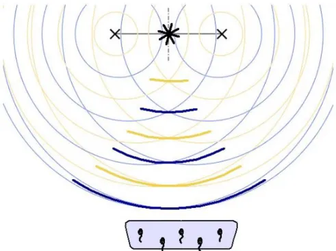
The second category consists of a specialized case, when the Mach radius is zero, associated with axial modes. This can be seen in Fig. 3, which depicts a generic test case for rotating
5
coherent monopole noise sources which are investigated from the near axial direction.
(Positioning microphones exactly on the axis will cancel out certain signals). As discussed above, the wave fronts propagate away from the rotating coherent noise sources, marked in the figure by 𝑥, interacting to form wave fronts of larger amplitude, marked in the figure by darker/thicker wave fronts, which appear to radiate from the Mach radius, marked in the figure by ∗, which in this case lays on the axis between the rotating coherent noise sources. In the figure, the axis of rotation is vertical, and the phased array of microphones is positioned such that the axis of rotation is almost normal to the plane of the array. Signals are recorded by the microphones, and when processing the data using most beamforming methods carried out in the stationary as well as rotating reference frame, a strong noise source will appear at the apparent noise source position located at the Mach radius (on the axis), to where the normal of the strong wave fronts can be traced, marked in the figure with by ∗. The literature provides a detailed explanation for why the Mach radius effects the beamforming results of rotating coherent noise sources [9], as well as making steps toward better explaining the results [11, 12] and overcoming these hardships for the special case when the Mach radius localizes the noise source to the axis [12, 13], but the literature does not yet provide information regarding a beamforming method designed specifically for localizing rotating coherent noise sources.
Fig. 3. Two rotating coherent noise sources investigated with a phased array of microphones. The wave fronts interact constructively and destructively to form a wave front of large amplitude, which appears to be radiating from the Mach radius.
3 SIGNIFICANCE OF THE DOPPLER EFFECT IN LOCALIZING ROTATING COHERENT NOISE SOURCES
It was shown in [13] that the information provided by the Doppler Effect is key to better understanding the beamforming results of rotating coherent noise sources and hence in developing beamforming methods for such noise sources. In order to understand why, let us first investigate two stationary coherent monopole noise sources, as seen in Fig. 1. Recording
6
the signal using one of the microphones in the array depicted in the figure, we can analyze the data using STFT analysis. In the simulation, the stationary coherent monopole noise sources are located on a circle having a diameter of 0.4m, spaced 180° apart. For the stationary case, these noise sources are not moving and are located in the plane of the page, as seen in Fig. 1.
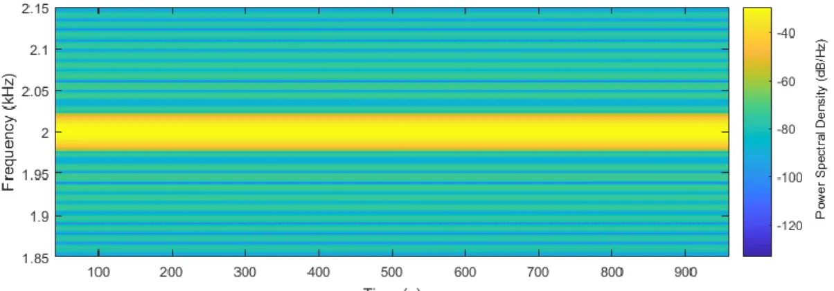
The phased array system is located at a distance of 3.5 m from the center of the circle, with the plane of the array being parallel to the plane of the circle. The sources are monopole point sources, emitting at a constant frequency of 2 kHz. The sampling frequency was 25 kHz. The STFT analysis was carried out for a window length consisting of 2048 data points, applying a Hamming window, and a 99% overlap. Figure 4 presents the spectrogram of this case. It can be seen that the signals from the two independent noise sources cannot be separated, as their frequencies align and hence amplitudes add together constructively. It can also be seen that the frequency is constant in time, as would be expected of stationary sources.
Fig. 4. STFT analysis of two stationary coherent monopole noise sources investigated with a single microphone.
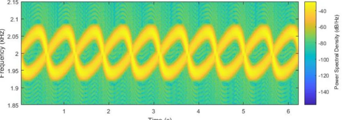
Next, we will investigate the case of 2 rotating coherent monopole noise sources, as seen in Fig. 2. In the simulation, the rotating coherent monopole noise sources are once again located on a circle having a diameter of 0.4m, spaced 180° apart. For this case, these noise sources are now rotating around the axis at a rate of 200rev/s, the plane of rotation being located in the plane of the page, as seen in Fig. 2. The phased array of microphones is located at a distance of 3.5 m from the center of the circle in a direction perpendicular to the axis of rotation. The sources are monopole point sources, emitting at a constant frequency of 2 kHz. The sampling frequency was 25 kHz. The STFT analysis was carried out for a window length consisting of 2048 data points, applying a Hamming window, and a 99% overlap. The Mach radii of certain BPF and interaction tones do not align with the axis, but are rather located at larger radii.
Investigating this test case with a microphone located on the sideline, the STFT can once again be carried out, the results of which are shown in Fig. 5. It can be seen that as compared to the case of stationary coherent noise sources, the frequency content of the results are much more complex. The Doppler Effect causes the frequency of the individual noise sources to oscillate around a given value. When the noise source is moving away from the microphone, the frequency decreases, and when it moves toward the microphone, it increases. The amplitudes also shift, though this is harder to see in the figure. Each noise source can be described by a somewhat morphed sinusoidal curve. In this case, since the two noise sources are offset by 180°, the two curves are also offset in time by half a rotation. As compared to the case of stationary noise sources, the two noise sources can now be distinguished from one
7
another. The Doppler Effect has therefore provided us with information for separating the two signals.
Fig. 5. STFT analysis of two rotating coherent monopole noise sources investigated with a single microphone.
If one where to investigate these two noise sources at any instant of time using a virtual rotating microphone which is moving together with the sources (compensating for everything, including the velocity of the medium between the sources and the microphone), one would arrive back at the case of two stationary coherent monopole noise sources, as described above in Fig. 4. The surplus of information provided by the Doppler Effect will therefore be lost.
This is in essence what is done in the method of Herold et al. [4] as well as that of Pannert et al. [3]. These methods therefore do not provide a good basis on which to build a beamforming method capable of localizing rotating coherent noise sources, even though it would be useful to take advantage of the CSM related opportunities. The method of Sijtsma et al. [1] on the other hand is somewhat different. The surplus information provided by the Doppler Effect is present in the signals recorded by the individual microphones, but is later lost during the de- Dopplerization step. This suggests two things. First of all, the ROSI method might be able to localize rotating coherent noise sources/might provide the basis for a method for the localization of rotating coherent noise sources. Second of all, the use of an array of stationary microphones is advantageous for the beamforming of rotating coherent noise sources, since the Doppler Effect helps separate the signals from individual noise sources in a microphones signal.
4 EVALUATION OF THE ROSI BEAMFORMING METHOD FOR ROTATING COHERENT NOISE SOURCES
The ROSI beamforming method is an extension of the Delay & Sum method for rotating sources [1]. The two methods differ mainly in that the ROSI method applies a so called de- Dopplerization step in order to place the rotating noise sources into a rotating reference frame, making them stationary for the purpose of carrying out the calculations. The positions and velocities of the possible noise sources are accounted for by correcting the time difference and amplitude data with regard to each receiver position. The corrected source signals are then processed using a beamforming method that corresponds with the Delay & Sum method. Let us examine the way in which the disturbances at the true source positions propagate from the sources to the receivers and then examine the way in which the ROSI method traces these measured pressure signals back to the sources in order to highlight points which are key in
8
understanding why the ROSI method might be able to localize rotating coherent noise sources whose Mach radii do not coincide with the axis.
4.1 Description of the measured pressure signal
In the ROSI method, the following expressions are used for describing the acoustic pressure signal 𝑝(𝒙, 𝑡), measured in a given receiver location 𝒙 at receiver time 𝑡 that is resulting from a given moving monopole noise source located at a source location 𝝃 at an emission time 𝜏 (see Eq. (1)). The equations presented below come from work presented in [1, 5, and 14].
𝑝(𝒙, 𝑡) = 𝜎(𝜏)
4𝜋{𝑐(𝑡−𝜏)+𝑄(𝒙,𝝃(𝜏),𝑡,𝜏)} (1)
Here 𝜎(𝜏) is the emitted signal from the source, 𝑐 is the speed of sound, and 𝑄 is the inner product which describes the Doppler shift of the signal reaching the receiver for a case having a flow velocity 𝑼, as seen in Eq. (2).
𝑄 =1
𝑐(−𝝃′(𝜏) + 𝑼)(𝒙 − 𝝃(𝜏) − 𝑼(𝑡 − 𝜏)) (2) The denominator of Eq. (1) is the transfer function between the source and the receiver, which will be marked here with 𝐹(𝒙, 𝝃(𝜏), 𝑡, 𝜏), as seen in Eq. (3).
𝐹(𝒙, 𝝃(𝜏), 𝑡, 𝜏) = 4𝜋{𝑐(𝑡 − 𝜏) + 𝑄(𝒙, 𝝃(𝜏), 𝑡, 𝜏)} (3)
The acoustic pressure measured by a given microphone of a phased array system 𝜒(𝑡) can therefore be described by Eq. (4).
𝜒(𝑡) = 𝜎(𝜏)
𝐹(𝒙,𝝃(𝜏),𝑡,𝜏) (4)
In Eq. (2), the distance that the sound propagates (𝒙 − 𝝃(𝜏) − 𝑼(𝑡 − 𝜏)) is multiplied by the Mach number with which the source is moving 𝑴 =1
𝑐(−𝝃′(𝜏) + 𝑼), taking into account the flow velocity. The positions and velocities in 𝑄 are given in vector form, and therefore when applying the Doppler shift for each individual noise source and receiver pair, the measured acoustic pressure signals will differ between receivers. This depends on the relative motion and positions of the given source and receiver, as well as their alignment with the flow velocity. This is very advantageous from a beamforming point of view, since the coherent noise sources will be incoherent, as perceived by the receivers. In a way, the coherent noise source signals are transformed by the Doppler Effect, providing us with a set of noise signals which can be distinguished from one another.
4.2 Description of the ROSI method
Let us examine how the ROSI method reconstructs the source signals for carrying out the localization of the noise sources. Rearranging Eq. (4), one arrives at Eq. (5), which provides
9
𝜎𝑛(𝜏), the reconstructed source signal from the nth microphone, where subscript 𝑛 refers to the nth microphone of the array.
𝜎𝑛(𝜏) = 𝜒𝑛(𝑡𝑛)𝐹(𝒙𝒏, 𝝃(𝜏), 𝑡𝑛, 𝜏) (5)
It can be seen that the transfer function 𝐹(𝒙𝒏, 𝝃(𝜏), 𝑡𝑛, 𝜏) was used to transform the signal from a given microphone position to the noise source position in the rotating reference frame, correcting the amplitude as well as arrival time, and hence phase and frequency of the signal.
Let’s examine 𝐹(𝒙𝒏, 𝝃(𝜏), 𝑡𝑛, 𝜏) in greater detail in Eq. (6).
𝐹(𝒙𝒏, 𝝃(𝜏), 𝑡𝑛, 𝜏) = 4𝜋{𝑐(𝑡𝑛− 𝜏) + 𝑄(𝒙𝒏, 𝝃(𝜏), 𝑡𝑛, 𝜏)} (6)
The first part of the transfer function within the brackets on the right hand side of the equal sign in Eq. (6) (𝑐(𝑡𝑛− 𝜏)) corrects for the phase shift of the signal resulting from the distance between the individual microphones and the investigated noise source positions. Applying this correction does not mean losing the information contained in the Doppler shift. The second part (𝑄(𝒙𝒏, 𝝃(𝜏), 𝑡𝑛, 𝜏)) corrects for the Doppler Effect, and therefore, after applying this transformation, the information contained in the Doppler shift is lost. Let’s look at this more closely in Eq. (7).
𝑄 =1
𝑐(−𝝃′(𝜏) + 𝑼)(𝒙𝒏− 𝝃(𝜏) − 𝑼(𝑡𝑛− 𝜏)) (7) It can be seen that the velocity of the source location 𝝃′(𝜏) plays a crucial role in this transformation. Therefore, if the velocity of the given source location is zero, then the Doppler Effect is not compensated for.
Following this transformation, Delay & Sum beamforming can be applied, since the signals of the incoherent noise sources which are truly located in a given point have been transformed to align in each time series of the various microphones. The following steps summarize the further steps of the ROSI method, which coincide with the Delay & Sum beamforming method. The reconstructed source signal 𝜎(𝜏) is attained in Eq. (8) by taking into account the reconstructed source signals from all 𝑁 microphones.
𝜎(𝜏) = 1
𝑁∑𝑁𝑛=1𝜎𝑛(𝜏) (8)
The beamforming values 𝐴 of the investigated potential source positions are then evaluated in the frequency domain by taking the Discrete Fourier Transform of 𝜎(𝜏), which is marked here by 𝜎̂(𝜏), and averaging, as described by Eq. (9).
𝐴 =1
2⟨|𝜎̂|2⟩ = 1
2𝑁2⟨∑𝑁𝑛=1∑𝑁𝑚=1𝜎̂𝑛𝜎̂𝑚∗⟩ (9) Here subscript 𝑚 refers to the mth microphone of the array, and the asterisk denotes the complex conjugate.
10 4.3 Evaluation of the ROSI method
As seen in the description provided in the above sections, the investigation of rotating coherent noise sources using a phased array of microphones results in signals being measured at the various microphone locations which are Doppler shifted. For any particular noise source, the time series of the signal recorded by each microphone will differ to some degree in phase, frequency, and amplitude, unless the noise source is located on the axis (where the rotational velocity is negligible and hence the Doppler shift is also negligible). More importantly, at any particular microphone position, the signals of each coherent rotating noise source will differ to some degree in phase, frequency, and amplitude. The ROSI method takes Eq. (4) and rearranges it in order to win back the original signal at the source position from each microphone in the array, which could also be worded as transforming the signal to a rotating reference frame, after which Delay & Sum beamforming can be carried out in order to determine whether a noise source is truly located in the given location or not [1]. This works wonderfully for incoherent noise sources, but is time consuming and the CSM provided opportunities cannot be taken advantage of.
Initially, it was believed that as a result of the inability of the Delay & Sum beamforming method to handle coherent noise sources, and since the information contained in the Doppler shifted data is lost during the de-Dopplerization step, the rotating coherent noise sources would not be localized to their true locations by the ROSI beamforming method, but would rather be localized to their Mach radii. During this investigation it was realized that this has not yet been looked in sufficient detail in research available in the literature. In [9, 11], the open rotors under investigation were investigated using frequency domain beamforming from a sideline position in the stationary reference frame. Therefore, the rotating coherent noise sources resulted in apparent noise sources being localized to their Mach radii. In [12, 13], both frequency domain beamforming as well as the ROSI beamforming method were applied in the investigation of rotating coherent noise sources which had a Mach radius of zero. As a result of the current investigation, it has been realized that investigating only the special case of 𝑧∗ = 0 in [12, 13] was inadequate for making general conclusions regarding the ability of the ROSI method to localize rotating coherent noise sources to their true positions. When investigating the on axis position with the ROSI method, the de-Dopplerization step does not alter the time signals of the microphones, since the velocity in that point is negligible.
Therefore, the wave front resulting from the constructive and destructive addition of the various rotating coherent noise sources will be traced back to the apparent noise source position on the axis. If the de-Dopplerization step is carried out for an azimuthal mode having a Mach radius larger than zero, it is not for certain whether the true noise source positions or the apparent noise source positions will dominate, since it is expected that the de- Dopplerization step will decrease the correlation between the various microphone signals at the Mach radius positions. Therefore, the use of the ROSI beamforming method for the investigation of rotating coherent noise sources having 𝑧∗ ≠ 0 needs to be further investigated. It is promising that the ROSI method might actually be applicable to rotating coherent noise sources whose Mach radii are not aligning with the axis. Regardless of the above stated findings, which are in themselves significant, a beamforming method for rotating coherent noise sources, especially one which can take advantage of the opportunities provided by the CSM would be useful.
11
5 PROPOSED METHODS FOR THE INVESTIGATION OF ROTATING COHERENT NOISE SOURCES
As discussed throughout the text, beamforming methods for rotating noise sources can be split into two main categories. The first category uses microphone data collected in the stationary frame of reference, while the second category uses virtual microphone data collected in a rotating frame of reference. From the first category, it would be useful to take advantage of the Doppler shifted data and of the fact that the array can be arbitrarily positioned. While from the second category, it would be useful to take advantage of opportunities provided by the CSM.
It was also discussed that STFT and DWT methods are appearing in the beamforming literature. Though these methods might not always be applied in order to allow for the investigation of unsteady phenomena, there is no reason why they should not be applied for this purpose. It would be advantageous to include these methods in order to improve the temporal resolution of the proposed methods. Two alternative methods for the investigation of rotating coherent noise sources are proposed below, though the details are not yet worked out in great detail for either method.
5.1 STFT or DWT followed by CSM based method
In the first approach, it is proposed that data be collected in the same way as done when applying the ROSI method. Therefore, a phased array system of choice should be set up in a stationary position of choice. Microphone signals should then be simultaneously sampled and recorded together with a once-per-rev signal. As with the ROSI method, it is suggested that the sampling frequency be high. In this case, this is necessary, because an STFT or DWT is being carried out on the data, and not because the time series is being manipulated (as in the ROSI method). The higher the sampling frequency, the more data points can be analyzed for each increment of time (one window length of data processed). The next step is the investigation of the data using STFT or DWT analysis. In this step it is important to minimize the length of the time which is being investigated in one time increment, while maximizing the number of samples which are being included in the analysis. In this way the temporal resolution can be improved, while the quality of the STFT or DWT is not affected. In order to reach the best results, it is most likely best to apply DWT instead of STFT, but this is the subject of future investigations. Once the data has been converted over to the frequency domain for each increment of time, then each of these increments of time can be processed using frequency domain beamforming, or any high-resolution beamforming method which is based on the CSM. The further development of this step is critical in the successful application of this method, since the creation and use of the CSM is rather complicated due to the Doppler Effect, which needs to be corrected for. Inevitably the processing time also needs to be assessed, as it will most likely be very long as compared to most other frequency domain based beamforming methods, which are not carried out for multiple increments of time. By processing the data in this way, the advantages of collecting data with stationary microphones, as well as the advantages associated with beamforming methods based on the CSM are all included in one method.
The first of the two proposed methods therefore consists of the following steps.
1) Conduct measurements of rotating coherent noise sources using a stationary phased array of microphones. (This step takes advantage of the Doppler Effect in order to distinguish noise sources from one another.)
12
2) Process the individual microphone signals using STFT or DWT analysis.
3) Apply frequency domain beamforming or any high-resolution beamforming method which is based on the CSM for every time increment under investigation.
In this step the CSM of the data for every investigated frequency band of every time increment investigated by STFT or DWT analysis needs to be created while keeping in mind that the Doppler Effect needs to be corrected for.
5.2 STFT or DWT followed by DWT based method
In the second method, it is proposed that the data be collected in the same manner as done when applying the ROSI method (and in the first proposed method). Therefore, a phased array system of choice should be set up in a stationary position of choice. Microphone signals should then be simultaneously sampled and recorded together with a once-per-rev signal. A high sampling frequency should once again be used. As stated earlier, this is necessary, since an STFT or DWT analysis is being carried out on the data. The next step is the investigation of the data using STFT or DWT analysis. Once the data has been converted over to the frequency domain for each increment of time, the spectrogram of the data should resemble what was seen in Fig. 5. As described earlier, each rotating tonal noise source is seen in the spectrogram as a somewhat morphed sinusoidal curve. Thanks to the Doppler Effect, individual rotating coherent noise sources can be distinguished from one another in the spectrogram, since they will be phase shifted. The curves of various rotating noise sources will also differ from one another in the spectrogram depending on the radial positions of the noise sources (extent of frequency shift) and their amplitudes (PSD magnitude). As pointed out in the first method proposed above, carrying out frequency domain beamforming for each increment of time will be rather tricky and time consuming. It is therefore proposed in the second method that the spectrogram be processed using something that resembles DWT analysis. As compared to DWT analysis as we know it, where the mother wave is defined by an amplitude as a function of time, the “amplitude” of the mother wave would in this case be frequency as a function of time, and the amplitude of the noise source which is described by the given mother wave could be determined based on the PSD amplitude of the spectrogram.
By processing the data in this way, the recorded rotating coherent noise source signals can be distinguished from one another, and can therefore be localized relatively quickly, but the advantages associated with beamforming methods which are based on the CSM are lost.
The second of the two proposed methods therefore consists of the following steps.
1) Conduct measurements of rotating coherent noise sources using a stationary phased array of microphones. (This step takes advantage of the Doppler Effect in order to distinguish noise sources from one another.)
2) Process the individual microphone signals using STFT or DWT analysis.
3) Apply DWT analysis to the spectrogram in order to localize noise sources in an investigated plane.
6 SUMMARY
This investigation aims at laying the foundation for a beamforming method which is designed specifically for the localization of rotating coherent noise sources. Since earlier investigations have shown that the Doppler Effect separates the various rotating coherent noise sources from one another in the microphone signals, the Doppler Effect plays a key role in the proposed methods. During the examination of various beamforming methods for
13
rotating noise sources made available in the literature, it was realized that the ROSI method might already be capable of localizing rotating coherent noise sources not localized to the axis of rotation. This unexpected, yet useful outcome will be further investigated in future research. At the end of the report, two proposed methods for investigating rotating coherent noise sources are outlined. Both methods record data with arbitrarily positioned stationary arrays of microphones and then carry out an STFT or DWT on the recorded data. In the next step the two methods differ, as the one will attempt to create a type of CSM for short increments of time, making it possible to use high resolution beamforming methods in the processing of the data, while the other will attempt to carry out a type of DWT analysis on the spectrogram created in the previous step. Both of these methods have potential advantages and disadvantages associated with them, and will be looked at in greater detail in future investigations.
ACKNOWLEDGEMENTS
The present investigation was supported by the Hungarian National Research, Development and Innovation Center under contract Nos. K 119943 and the János Bolyai Research Scholarship of the Hungarian Academy of Sciences. The work relates to the scientific programs “Development of quality-oriented and harmonized R+D+I strategy and the functional model at BME” (Project ID: TÁMOP-4.2.1/B-09/1/KMR-2010-0002) and “Talent care and cultivation in the scientific workshops of BME” (Project ID: TÁMOP-4.2.2/B-10/1- 2010-0009).
REFERENCES
[1] P. Sijtsma, S. Oerlemans, and H. Holthusen. “Location of rotating sources by phased array measurements.” AIAA 2001-2167, 2001. 7th AIAA/CEAS Aeroacoustics Conference, Maastricht, Netherland, May 2001.
[2] O. Minck, N. Binder, O. Cherrier, L. Lamotte, and V. Budinger, “Fan noise analysis using a micro-phone array.” 2012. International Conference on Fan Noise, Technology
& Numerical Methods, Senlis, France, 18-20 April, 2012.
[3] W. Pannert, and C. Maier. “Rotating beamforming – motion-compensation in the frequency domain and application of high-resolution beamforming algorithms.” Journal of Sound and Vibration, Vol. 333, Issue 7, 1899-1912, 2014.
[4] G. Herold, and E. Sarradj. “Microphone array method for the characterization of
rotating sound sources in axial fans.” Noise Control Engineering Journal, Vol. 63, Issue 6, 546-551, 2015.
[5] L. Koop. “Beamforming methods in microphone array measurements. Theory, practice and limitations.” VKI Lecture Series 2007-01. 87-166, 2007.
[6] W. Ma, and X. Liu, “Improving the efficiency of DAMAS for sound source localization via wavelet compression computational grid.” J. Sound Vib., 395, 341-353, 2017.
doi:10.1016/j.jsv.2017.02.005.
[7] J. Benesty, J. Chen, and C. Pan, “Fundamentals of differential beamforming.” Springer, 2016.
[8] M. J. T. Smith. “Aircraft noise.” Cambridge University Press, 1989.
14
[9] Cs. Horváth, E. Envia, G.G. Podboy. “Limitations of phased array beamforming in open rotor noise source imaging.” AIAA Journal, Vol. 52, No. 8, 1810-1817, 2014.
[10] A. B. Parry and D. G. Crighton. “Prediction of counter-rotation propeller noise.” AIAA- 89-1141, 1989. 12th AIAA Aeroacoustics Conference, San Antonio, Texas, April 1989.
[11] Cs. Horváth. “Beamforming investigation of dominant counter-rotating open rotor tonal and broadband noise sources.” AIAA Journal, Vol. 53, No. 6, 1602-1611, 2015.
[12] Cs. Horváth, B. Tóth, P. Tóth, T. Benedek, and J. Vad. “Reevaluating noise sources appearing on the axis for beamform maps of rotating sources.” Paper 013, 2015.
International Conference on Fan Noise, Technology & Numerical Methods, Lyon, France, 15-17 April, 2015.
[13] Cs. Horváth, B. Tóth. “Separating apart the contributions from multiple tonal noise sources which are localized to the Mach radius.” BeBeC-2016-D16. URL
http://www.bebec.eu/Downloads/BeBeC2016/Papers/BeBeC-2016-D16.pdf,
Proceedings on CD of the 6th Berlin Beamforming Conference, February 29-March 1, 2016.
[14] P. Sijtsma. “Using phased array beamforming to locate broadband noise sources inside a turbofan engine.” NLR-TP-2006-320. National Aerospace Laboratory Executive summary, 2006.