Identifier and the Virtual Rotating P

(1)

Abstract

The aim of this paper is to present two acoustic beamforming methods developed for rotating sources, namely the Rotat- ing Source Identifier (ROSI) and the Virtual Rotating Array method (VRAM). These were applied onto a series of simulated test cases, and their behaviour was analysed. Both methods were able to localise the source reliably. However, the source strength was found to depend on the number or microphones when VRAM was applied. This phenomenon was quantified and an approximate formula was given providing the minimum number of microphones required to reach a certain amplitude error. Beamwidth and side lobe suppression were found to agree between the two methods, meaning that the way rotation is handled does not significantly affect the point spread func- tions. The computational cost of ROSI was two to three orders of magnitude higher than that of VRAM. The results show that both methods are applicable for the beamforming analysis of rotating sound sources. However, in case of VRAM, the num- ber of microphones has to be chosen carefully to obtain reli- able amplitude results.

Keywords

beamforming, rotating sound source, phased array microphone, Rotating Source Identifier, Virtual Rotating Array method

1 Introduction and objectives

The noise emitted by machinery is an increasingly important concern, due to its adverse effects on people. Noise reduction is therefore of paramount importance. However, the sources of noise are often unknown. Acoustic beamforming is a technology that localizes sound sources based on measurements carried out with an array of microphones [1]. It is widely applied for stationary sources to analyse and investigate noise genera- tion mechanisms with the aim of reducing noise.

Rotating machines are significant sources of noise, too, therefore they are often investigated using beamforming techniques. Turbomachinery are traditionally of great interest due to the strict air traffic regulations [2, 3]. Wind turbines are similarly important, as they are becoming more widespread [4].

More recently, low-speed axial fans have been studied as well [5-8]. These machines emit little noise compared to e.g. turbo- fans, however, they are often used in the close vicinity of people, therefore their noise should be reduced as well.

It is then important to deal with rotating noise sources, however, their investigation is made difficult by the continuously changing source–receiver distances, resulting in the apparent change of the received frequency, termed the Doppler effect.

Nevertheless, there are several beamforming methods developed for rotating sources. Approaches exist both in the time domain [9], and in the frequency domain [6, 10-12]. Each of them has different advantages, application criteria and limitations.

Microphone array methods are often analysed and compared against each other [13, 14]. The literature however rarely treats the comparison of methods for rotating sources, probably due to their sometimes mutually exclusive application criteria. Reference [15] reports such a work, where the virtual rotating array method [6] and the frequency domain rotation compensation technique [11, 12] is used to characterise the sound sources in an axial fan.

Time-domain de-Dopplerisation is not applied there, however, and duct modes are considered, as the case involves a ducted fan. The aforementioned three groups of methods are compared in [16], with interesting results regarding the performances of the methods applied together with deconvolution methods, however, little information is available about the original beamforming results.

1 Department of Fluid Mechanics, Faculty of Mechanical Engineering,

Budapest University of Technology and Economics, H-1111 Budapest, Bertalan Lajos u. 4-6, Hungary

* Corresponding author, e-mail: tothbence@ara.bme.hu

Comparison of the Rotating Source Identifier and the Virtual Rotating Array Method

Gábor Kotán

¹

, Bence Tóth

^1*

, János Vad

¹

Received 26 June 2017; accepted after revision 25 June 2018

PP Periodica Polytechnica Mechanical Engineering

OnlineFirst (2018) paper 11194 https://doi.org/10.3311/PPme.11194 Creative Commons Attribution b research article

(2)

The objective of this paper is to analyse some methods developed for rotating sources. Summarise their requirements, advantages and drawbacks, then apply them on the same test cases. Examine the results, and draw conclusions based on them, using quantitative parameters characterising a beamform map. This is to provide some preliminary information to aid designing beamforming experiments on rotating sound sources.

First, the applicable methods are introduced shortly.

Second, the relevant methods are applied to localise a single rotating monopole source, whose angular velocity, and signal frequency are varied. The number of microphones in the array is changed, as well. The beamform maps are analysed first visually, then quantitatively, considering the main lobe level at the location of the source, the beamwidth, and the side lobe suppression. Computational costs are analysed, too.

Special attention is paid to VRAM, and the beamform level of the localised source. Finally, conclusions are drawn that highlight the differences between the methods, and give useful advice regarding their application possibilities.

2 Methods for rotating sources

Three fundamentally different methods have been proposed to localise rotating sources. These are shortly summarised in this section, together with their application criteria, and fore- seeable advantages and disadvantages. Such special methods are required, as conventional frequency-domain beamforming is not able to handle moving cases, because of the relative change of receiver position, when viewed from the source.

2.1 Rotating Source Identifier

The Rotating Source Identifier (ROSI) method was pro- posed in [9]. It works in the time domain, and its general idea is to calculate the beamforming result on grid points that rotate together with the target.

First, a grid point is chosen. Then, a uniformly spaced emission time series is created, using the length and the sampling frequency of the measurement. For each emission time instant, the rm,n distance between the investigated grid point n and each microphone m is calculated, making use of the angular position of the target. Using the speed of sound a, this gives the times of flight of uniformly emitted sound pulses from the selected grid point. Its time-dependence is what causes the Doppler effect.

Adding up the emission times and the times of flight, the τ arrival times are obtained, shown in Eq. (1).

τm n

t t m n

r t

, a

( ) , ( )

.

= +

These are not uniformly distributed any more, therefore the pressure signal p_m

( )

t of each microphone is interpolated onto the τ non-uniform arrival time vector, thus p_m

( )

t is obtained.

In this step the amplitude variation is taken into account as well. The resulting sound pressure vector is then treated as the

noise emitted from the investigated grid point, at the original, uniformly spaced t emission time instants. This way the rotation effects are removed, and from that, the beamform level at the investigated point can be determined. The procedure is repeated for all grid points.

ROSI is able to take rotation effects into account. It can be applied for non-uniform angular velocity and arbitrary array geometry. However, due to the time domain calculations, the method is very resource-consuming, and since there is no cross spectral matrix to describe the complete source field, a large number of deconvolution methods cannot be applied.

2.2 Virtual rotating array method

Another method, termed Virtual Rotating Array method (VRAM) was proposed in [6]. Earlier, a similar algorithm was applied in [10] for a ducted fan. In these methods, the funda- mental idea is to create a virtual array, rotating together with the target. These methods originally require the microphones to be arranged along one or more rings with uniform angular separation. (This requirement was removed in [17].) The axis of the array must also be identical to the axis of revolution of the target.

A virtual array of microphones is imagined as rotating together with the target. First, a virtual microphone of index m is chosen. Its angular position in time is calculated, which is then used to determine the index of the microphones in the real array preceding (m⁻) and following (m⁺) the virtual microphone m at each time step. They are obtained using Eqs. (2) and (3), respectively. In these equations, the angular separation of the microphones is α =2π M,   means the floor operation, and mod M means the remainder after division by M.

m t m

t

− = ^ +

( )

₋ M

 













+

( ) ϕ mod

α 1 1

m t m

t

+ = ^ +

( )

M

 













+

( ) ϕ mod .

α 1

Finally, the signal at the virtually rotating microphone m is obtained by linearly interpolating the signals of microphones m⁻ and m⁺, weighted by the distances, as shown in Eq. (4).

m m m

p

( )

t ⁼s p⁻ ⁻

( )

t ⁺s p⁺ ⁺

( )

t ^.

The weights of the following and the preceding microphone signals are given in Eq. (5) and (6), respectively.

s t

t t

+ =

( )

−

( )

 

 ( ) ϕ

α ϕ

α

s⁻( )t = −1 s⁺( )t .

This procedure is repeated for each t time instant and each m microphone. This way, following a Fourier transform, the (1)

(2)

(3)

(4)

(5)

(6)

(3)

acoustic pressure p is obtained, as if the microphones were rotating together with the target of beamforming. From then on, a cross spectral matrix C can be constructed, and conventional beamforming can be carried out, as shown in Eq. (7) [1].

†

zn =w C w_n _n

In Eq. (7), w_n is the steering vector, describing the propagation of sound from grid point n to each microphone, while zn

is the result of beamforming at the n-th grid point. ^† denotes the complex conjugate transpose operator. In the present investigation, zn is written in a level form, denoted by Lb in Eq. (8).

The normalisation factor used here is the threshold of hearing:

p0 = 2 × 10⁻⁵ Pa. The source map values are given in this quan- tity for both ROSI and VRAM.

L z

b p

=¹⁰ 10 n

[ ]

0

log 2 dB .

Using this algorithm, the effects of rotary motion can be removed. Afterwards, the problem is reduced to a simple case with steady sources. Therefore all the methods developed for steady beamforming can be applied, including deconvolution approaches. The procedure is suitable for varying angular velocity, too, similarly to the ROSI method, but it requires a uniformly distributed circular array, placed perpendicularly the source rotation axis. This method is investigated in detail, as well.

2.3 Series expansion method

For the sake of completeness, it should be noted that besides ROSI and VRAM, a third kind of method also exists for rotating sources, proposed in [12] based on the work in [11]. This method is based on writing the Green's function for the rotating source in a spherical coordinate system. Utilizing the symmetry, this method works completely in the frequency domain and allows the application of deconvolution methods. It can however only be applied in case of an axially symmetric measurement setup, with a ring-shaped microphone array and a constant speed of revolution. Due to the complexity of the formulation, this method is excluded from the present investigations. The comparative analysis of this method optionally forms the subject of future work.

3 Methodology

The selected methods were compared using synthetic sources.

This is common practice when beamforming array methods are analysed [13, 14, 18]. An in-house algorithm was used to generate the required sound signals, first creating the emitted noise vector, being significantly oversampled compared to the sampling frequency of the final signal. Then, these signals were numerically propagated to each microphone using the time-de- pendent source – receiver distance obtained from the prescribed motion. The recorded pressure value for each of the oversampled source values was generated, using a far-field, free space monopole propagation model. This resulted in a non-uniformly

distributed pressure time history at each microphone, that was re-sampled to the uniform sampling frequency of the final signal using spline interpolation. Beamforming was carried out with an in-house ROSI code, reported in [19]. This program was extended by the authors to incorporate VRAM.

The applied weight vector was chosen to conform with pre- vious investigations reported in literature [5, 20, 21]. One ele- ment of this vector is shown in Eq. (9).

m

m n

r M

i r c

wn

( )

⁼ ⁴^π ^, ^exp

(

⁻^ω ^,

)

^.

For our investigation, test cases relevant for industrial measurements on low speed axial fans were considered. The ambient pressure was 10⁵ Pa, the ambient temperature 293.15 K, the ratio of specific heats 1.4, and the specific gas constant 287 J kg^-1 K^-1.

One source was investigated, its location being representative of the fan tip radius, placed at the coordinates x = 1, y = 0.2 m.

The reason for investigating just one source is the high computational demand of ROSI. This was deemed acceptable, as the source represents a point on the tip radius, often of interest in an axial fan [21]. Furthermore, the angular location has little rele- vance, if the number of microphones M is large enough, being a further reason for investigating only one source position.

Due to the requirements of the VRAM method, all arrays consisted of microphones being distributed along a circle, whose centre falls onto the axis of revolution of the source.

The diameter of the microphone array was 1 m.

Beamforming expressions were evaluated on a rectangular grid with 5 mm spacing. The distance between the source plane and the array plane was Z = 1 m. The final sampling frequency was 44 100 Hz. For the calculation of the cross spectral matrix, the Welch method [22] was followed: blocks consisting of 1024 data points were used with von Hann windows, overlap- ping by 50 %. In each case, the diagonal elements of the matrix were removed, similarly to the method in [18]. This is to conform with usual measurement settings, however, it was found to have negligible effect in the present case due to the presence of only one synthetic source.

Preliminary tests were carried out to determine the applied sample lengths. 0.1 s was found acceptable, providing the same results as a sample of 1 s in case of both methods. Thus 0.1 s samples were applied for ROSI in order to reduce the computational cost. When the computational requirements were considered, VRAM was also evaluated on samples of 0.1 s length, to get comparable results. However, when the amplitude of the source was investigated, samples of 1 s were used for VRAM.

The investigated nominal signal frequencies were f = 1, 2, 3, 4, 5 kHz; always modified to fall onto a discrete Fourier frequency. The speed of revolution of the rotor was varied between Ω = 10 1/s and 30 1/s in steps of 5 1/s. The number of microphones M was also varied between 12 and 80 in steps of 8 for VRAM, while for ROSI 24, 56, 64 and 80 were used, again (7)

(8)

(9)

(4)

to reduce the computational demand. The source strength was set in a way that in the absence of rotation, a beamform level of Lb = 0 dB was obtained in the map.

Beamform maps were created, and from those, the main lobe width, the side lobe suppression, and the maximum strength were extracted, and compared in case of the two methods. The results are presented and discussed below.

4 Beamforming results

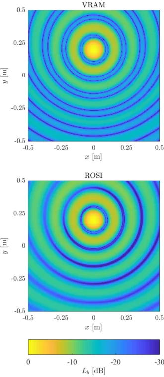
Fig. 1 depicts a source map from each method with equal dynamic ranges. These were obtained with the same parameters:

f = 3 kHz, Ω = 20 1/s, M = 64. Comparing the figures, one can see that both methods have localised the source successfully, and the strength estimates are very similar, as well, meaning that both methods are applicable. The point spread functions are also very similar, reported also in [16]. This observation was found true for all the investigated cases. Thus removing the rotation effects does not influence the beamforming part significantly; the point spread functions are similar to what would be obtained with conventional beamforming in case of stationary sources. This means that results on stationary sources could be used to judge the goodness of microphone layouts for ROSI or VRAM, as well.

Due to the similarity between the point spread functions, the width of the main lobe, and the side lobe strength all agree well, meaning that the achievable spatial resolution and the dynamic range are similar, too. This result was observed in all cases, meaning that the two methods give equivalent results from the point of view of beamforming. It should be noted however, that since VRAM uses a frequency-domain beamforming formulation, a multitude of deconvolution methods can be applied there to enhance the beamforming map, e.g. CLEAN-SC [23].

Comparison between some methods can be found in [16].

As noted before, the maximum Lb of the maps agrees well, too, in the reference case M = 64. However, VRAM was found to underestimate Lb when M was low. This probably results from the fact that as M decreases, the angular separation α of the microphones increases, and thus the results of the interpolation in Eq. (4) may degrade.

In case of ROSI, as noted before, only some practically relevant microphone numbers of M = 24, 56, 64 and 80 were investigated. In these cases, a constant deviation of about -0.07 dB from the ideal Lb was observed. This however did not depend on the number of microphones. Its origins were not investigated, since due to its weakness, it is unlikely to be of interest in measurement scenarios.

Fig. 2 shows the ∆Lb error relative to the ideal Lb value in case of VRAM. It can be seen that for increasing M values, ∆Lb

tends towards zero, as expected, however, for decreasing M, the magnitude of ∆Lb increases, and at a very low M of 12, an error above 2 dB is possible. The degradation of the beamform maps is shown in [16], but no numerical results are presented there. It should be noted that the location of the source was

successfully determined even with M = 16, while at M = 12, only a negligible position error was obtained.

The above result can be important when designing a microphone array: one has to consider the permissible uncertainty in L_b when choosing M. This can be achieved based on Fig. 3, showing the required M as a function of the amplitude error.

These results can be approximated well with a remarkably simple function, shown in expression (10), and in Fig. 3 with a dashed line. Using this approximate formula, the required M can readily be determined.

M

Lb

≈ 20

∆ .

Fig. 1 Source maps at f = 3 kHz, M = 64, Ω = 20 1/s

(10)

(5)

It should be noted that the numerical results are only valid for the present case, with f = 3 kHz, Z = 1 m, Ω = 20 1/s, a source radius of 0.2 m and an array diameter of 1 m. Nevertheless, since these parameters were chosen based on real-life axial fan measurements, they can be applied as guidelines for other similar cases. Investigating this phenomenon with other parameters forms the subject of future work.

Interestingly, varying Ω was not found to affect the L_b values in the maps. Changing the frequency was found to have a minor effect on both ROSI and VRAM results. Increasing f from 1 kHz to 5 kHz resulted in L_b being decreased by about 0.25 dB with M = 64. This effect can probably be attributed to the degrada- tion in interpolation as the wavelengths decrease relative to the microphone separations in case of VRAM, however, its magnitude is small and would not be noticeable in a real measurement.

5 Beamforming spectra

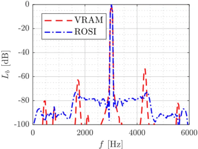
Fig. 4 depicts the spectral distribution of L_b at the location of the source. One can observe that both methods have successfully identified the source at 3 kHz with the amplitude reaching very close to the real one. All other spectral peaks are significantly weaker than the main source, indicating that the methods per- form as expected. Nevertheless, the trends of the methods appear different: ROSI has a wider range with nearly constant values

surrounding the real signal frequency, besides which the results fall. VRAM on the other hand has lower overall values, with some secondary peaks: a lower frequency one appearing at about fl =1700 Hz and a higher frequency one close to fh = 4300 Hz.

Fig. 4 ROSI and VRAM L_b spectra at the source position (M = 64, Ω = 20 1/s, f = 3 kHz)

The aforementioned peaks were found in all VRAM results and some of their properties were analysed. The f_l ≈ f − 1300 Hz and fh ≈ f + 1300 Hz relationship was found regardless of the signal frequency f . When M increases, fl was found to decrease, while fh was found to increase, both in a linear manner.

They exhibit a similar trend when Ω was varied.

At these fl and fh frequencies, the beamforming maps show secondary sources localised in the same direction from the ori- gin, as the real source, but on a different radius. These radii were found to be linear in terms of f , M , and Ω, as well.

They exhibited no dependence on Z or the array diameter.

In the present work, these secondary sources were not investigated in more detail.

6 Computational cost

Fig. 5 shows the processing time T required by each algorithm as a function of M. This was measured in the GNU Octave environment running on a personal computer with an Intel Core i5 processor.

The most important conclusion is that ROSI has two to three orders of magnitude higher computational cost in the present range of parameters than VRAM. In Ref. [16], VRAM was found to be 350 times faster than ROSI, being in good agreement with the present findings. The exact result depends on implementation details, but it is nevertheless clear, that VRAM is significantly faster than ROSI. Furthermore, as the number of microphones increases, the advantage of VRAM further grows, since T is about proportional to M for VRAM, but for ROSI, this is a higher degree dependence.

ROSI was also found to have T directly proportional to the number of grid points, while in case of VRAM a more moderate dependence was discovered.

Fig. 2 Beamform peak against the number of microphones

Fig. 3 Beamform peak against the number of microphones

(6)

The reason for the speed of VRAM is that interpolation of the sound pressure signals has to be carried out only once for each microphone, which is followed by conventional beamforming.

For ROSI however, the distances have to determined for each time step, each grid point and each microphone, followed by the interpolation, taking considerable time.

7 Conclusions

The paper has demonstrated two of the available methods for beamforming on rotating sources: ROSI and VRAM.

It contributes to the beamforming literature by providing some results of numerical experiments, aiding in determining the appropriate method for microphone array measurements on rotating sources. Besides visual observation of the beamform map, the beamform level, the beamwidth, and the side lobe suppression were investigated. These parameters were gener- ally found to be in good agreement between the methods.

A previously not reported dependence was found on the number of microphones: as M decreases, the Lb beamforming value obtained by VRAM decreases from the real value. This may be an important concern when designing an array for rotating sources, therefore an approximate formula was provided, that allows determining the required number of microphones M for a prescribed allowable amplitude uncertainty.

The computational cost of the two methods was examined, as well. Results similar to those reported in [16] were obtained, indicating that ROSI has a two to three orders of magnitude higher computational requirement than VRAM.

The results show that the application of VRAM is benefi- cial, as it has low computational requirements, but identifies the sources well. Its results are acceptable if the number of microphones is large enough. The required ring shaped array geometry may be a drawback, as it usually has to be manufac- tured specially for the method.

ROSI is able to localize and quantify the sources, as well. It is very robust, giving accurate results even for a small number of microphones. But due to the time-domain procedure, the major- ity of deconvolution methods can not be used. Furthermore, its computational demands are significantly higher, than those of VRAM. It should be noted however, that ROSI can be applied for any array geometry, therefore it does not require manufac- turing an array specifically for the analysis of rotating sources.

Some array geometries are known to reduce side lobes and provide better source maps, even without deconvolution algorithms [24]. In the present case, a well-optimised array could reduce side lobe strength by about 10 dBs. The application of ROSI onto data obtained with a ring array is therefore not practical in a real-world scenario, it is only presented herein to provide a basis on which the methods can appropriately be compared.

Nomenclature Abbreviations

ROSI Rotating Source Identifier VRAM Virtual Rotating Array Method

Variables

a speed of sound

C cross-spectral matrix

f frequency

i −1

L_b beamform level

n grid point index

N number of grid points

m microphone index

M number of microphones

p sound pressure

p vector of recorded pressure signals



p interpolated sound pressure

r distance

s interpolation weight

t time

T runtime

x horizontal coordinate in the array plane y vertical coordinate in the array plane

w steering vector

z result of beamforming

Z distance between array and target grid α microphone angular spacing

Fig. 5 Runtime against the number of microphones. Sample length: 0.1 s.

Number of grid points: 161 × 161

(7)

φ angular location

λ wavelength

τ reception time

ω circular frequency

Ω angular velocity

Indices

− preceding microphone

+ following microphone

0 refers to the threshold of hearing

h higher

l lower

Acknowledgements

This work has been supported by the Hungarian National Research, Development and Innovation Centre under contract No. K 112277.

The work relates to the scientific programs "Development of quality-oriented and harmonized R+D+I strategy and the functional model at BME" (Project ID: TÁMOP- 4.2.1/B-09/1/KMR-2010-0002) and "Talent care and cul- tivation in the scientific workshops of BME" (Project ID:

TÁMOP-4.2.2/B-10/1-2010-0009).

The project has been supported by the ÚNKP-16-3-I.

New National Excellence Program of the Ministry of Human Capacities.

The authors acknowledge that the new scientific results published in this paper are the independent results dedicated to Bence Tóth.

References

[1] Dougherty, R. P. "Beamforming In Acoustic Testing." In: Mueller, T.

J. (ed.) Aeroacoustics Measurements. Experimental Fluid Mechanics.

(pp. 62-97), Springer, Berlin, Heidelberg, Germany. 2002.

https://doi.org/10.1007/978-3-662-05058-3_2

[2] Sijtsma, P. "Using Phased Array Beamforming to Identify Broadband Noise Sources in a Turbofan Engine." International Journal of Aero- acoustics. 9(3), pp. 357-374. 2010.

https://doi.org/10.1260/1475-472X.9.3.357

[3] Kennedy, J., Eret, P., Bennett, G., Sopranzetti, F., Chiariotti, P., Castel- lini, P., Finez, A., Picard, C. "The application of advanced beamforming techniques for the noise characterization of installed counter rotating open rotors." In: 19st AIAA/CEAS Aeroacoustics Conference, Berlin, Germany, May 27-29, 2013.

https://doi.org/10.2514/6.2013-2093

[4] Ramachandran, R. C., Raman, G., Dougherty, R. P. "Wind turbine noise measurement using a compact microphone array with advanced deconvolution algorithms." Journal of Sound and Vibration. 333(14), pp. 3058-3080. 2014.

https://doi.org/10.1016/j.jsv.2014.02.034

[5] Benedek, T., Vad, J. "An industrial onsite methodology for combined acoustic-aerodynamic diagnostics of axial fans, involving the phased array microphone technique." International Journal of Aeroacoustics.

15(1-2), pp. 81-102. 2016.

https://doi.org/10.1177/1475472X16630849

[6] Herold, G., Sarradj, E. "Microphone array method for the characterization of rotating sound sources in axial fans." Noise Control Engineering Journal. 63(6), pp. 546-551. 2015.

https://doi.org/10.3397/1/376348

[7] Zenger, F. J., Herold, G., Becker, S., Sarradj, E. "Sound source localiza- tion on an axial fan at different operating points." Experiments in Fluids.

57(8), p. 136. 2016.

https://doi.org/10.1007/s00348-016-2223-8

[8] Minck, O., Binder, N., Cherrier, O., Lamotte, L., Pommier-Budinger, V.

"Fan noise analysis using a microphone array." In: Fan 2012 - Interna- tional Conference on Fan Noise, Technology and Numerical Methods, Senlis, France, Apr. 18-20, 2012.

[9] Sijtsma, P., Oerlemans, S., Holthusen, H. "Location of rotating sources by phased array measurements." In: 7th AIAA/CEAS Aeroacoustics Conference and Exhibit, Maastricht, The Netherlands, May 28-30, 2001.

https://doi.org/10.2514/6.2001-2167

[10] Dougherty, R. P., Walker, B. E. "Virtual Rotating Microphone Imaging of Broadband Fan Noise." In: 15th AIAA/CEAS Aeroacoustics Con- ference (30th AIAA Aeroacoustics Conference), Miami, Florida, USA, May 11-13, 2009.

https://doi.org/10.2514/6.2009-3121

[11] Lowis, C. R., Joseph, P. F. "Determining the strength of rotating broadband sources in ducts by inverse methods." Journal of Sound and Vibra- tion. 295(3), pp. 614-632. 2006.

[12] Pannert, W., Maier, C. "Rotating beamforming − motion-compensation in the frequency domain and application of high-resolution beamforming algorithms." Journal of Sound and Vibration. 333(7), pp. 1899-1912. 2014.

[13] Herold, G., Sarradj, E. "Performance analysis of microphone array methods." Journal of Sound and Vibration. 401, pp. 152-168. 2017.

[14] Ehrenfried, K., Koop, L. "Comparison of Iterative Deconvolution Al- gorithms for the Mapping of Acoustic Sources." AIAA Journal. 45(7), pp. 1584-1595. 2007.

https://doi.org/10.2514/1.26320

[15] Caldas, L. C., Greco, P. C., Pagani, C. C., Baccalá, L. A. "Comparison of Different Techniques for Rotating Beamforming at the University of Sao Paolo Fan Rig Test Facility." In: 6^th Berlin Beamforming Conference 2016, Berlin, Germany, Feb. 24-25, 2016.

[16] Herold, G., Ocker, C., Sarradj, E., Pannert, W. "A Comparison of Mi- crophone Array Methods for the Characterization of Rotating Sound Sources." In: 7^th Berlin Beamforming Conference 2018, Berlin, Germany, March 5-6, 2018.

[17] Tóth, B., Kalmár-Nagy, T., Vad, J. "Rotating Beamforming with Uneven Microphone Placements." In: 7^th Berlin Beamforming Conference 2018, Berlin, Germany, Mar. 5-6, 2018.

[18] Herold, G., Sarradj, E. "An Approach to Estimate the Reliability of Mi- crophone Array Methods." In: 21st AIAA/CEAS Aeroacoustics Confer- ence, Dallas, Texas, USA, June 22-26, 2015.

https://doi.org/10.2514/6.2015-2977

[19] Benedek, T., Tóth, P. "Beamforming measurements of an axial fan in an industrial environment." Periodica Polytechnica Mechanical Engineering.

57(2), pp. 37-46. 2013.

https://doi.org/10.3311/PPme.7043

[20] Benedek, T., Vad, J. "Study on the Effect of Inlet Geometry on the Noise of an Axial Fan, With Involvement of the Phased Array Microphone Tech- nique." In: ASME Turbo Expo 2016: Turbomachinery Technical Confer- ence and Exposition, Seoul, South Korea, June 13-17, 2016.

https://doi.org/10.1115/GT2016-57772

(8)

[21] Tóth, B., Vad, J. "Algorithmic localisation of noise sources in the tip re- gion of a low-speed axial ow fan." Journal of Sound and Vibration. 393, pp. 425-441. 2017.

[22] Welch, P. "The use of fast Fourier transform for the estimation of power spectra: A method based on time averaging over short, modified peri- odograms." IEEE Transactions on Audio and Electroacoustics. 15(2), pp. 70-73. 1967.

https://doi.org/10.1109/TAU.1967.1161901

[23] Sijtsma, P. "CLEAN Based on Spatial Source Coherence." International Journal of Aeroacoustics. 6(4), pp. 357-374. 2007.

https://doi.org/10.1260/147547207783359459

[24] Underbrink, J. R. "Aeroacoustic Phased Array Testing in Low Speed Wind Tunnels." In: Mueller, T. J. (ed.) Aeroacoustics Measurements. Ex- perimental Fluid Mechanics. (pp. 98-217), Springer, Berlin, Heidelberg, Germany. 2002.

https://doi.org/10.1007/978-3-662-05058-3_3