1
ROTATING BEAMFORMING WITH UNEVEN MICROPHONE PLACEMENTS
Bence Tóth, Tamás Kalmár-Nagy and János Vad
Department of Fluid Mechanics, Faculty of Mechanical Engineering, Budapest University of Technology and Economics
H-1111 Hungary, Budapest, Bertalan Lajos street 4-6
ABSTRACT
Investigation of rotating sound sources is a difficult task for beamforming. One way to solve it is to construct virtual arrays that rotate together with the target. This is achieved by the Virtual Rotating Array Method, that requires the microphones to be arranged on the circumference of a circle. Furthermore, the angular distances of the neighbouring microphones have to be constant. The current paper extends this method to handle uneven microphone placements. The motivation behind this is that in case of conventional beamforming, usually uneven microphone-to-microphone distances are preferred. Numerical studies have been carried out to determine the main lobe width and the side lobe suppression of some arrays, where the microphone angular location are described by a power law with varying exponent. The results suggest that out of these possibilities, the equidistant array performs best. The sensitivity of VRAM to microphone angular position error was tested as well, which was found to be negligible in case of an array with 32 microphones.
2
1 INTRODUCTION
Rotating machinery, e.g. fans, gas turbines etc. are often significant sources of noise, and their investigation is an important step to reduce these emissions. Beamforming [1] is a useful tool to discover the spatial distribution of acoustic sources. Conventional beamforming however cannot be applied when the sources move, due to the time-varying source-receiver distances.
The resultant varying time of flight, and the frequency shift, has to be accounted for in order to reconstruct the source field on the rotating target.
One way of solving these problems is by applying the virtual rotating array method (VRAM) [2], [3]. Here the basic idea is to construct a virtual microphone array that rotates together with the target, by interpolating the measured sound pressure data. The advantages of the approach are as follows. Since the problem is reduced to the case of a stationary source, conventional beamforming, advanced deconvolution methods, and all the recent developments in beamforming methods can be applied. Runtime is favourable when compared to methods that operate in the time domain, such as the Rotating Source Identifier [4]. The reduction in processing time can be on the order of a hundred. Furthermore, the implementation is fairly straight-forward. Besides that, varying speeds of revolution can be handled, as well. A limitation is that the formulation in [3], requires a circular array with uniform microphone spacing, the array being placed perpendicularly to the axis of rotation, with the array centre falling onto the axis. These are manageable requirements, and the method has been successfully used to investigate fans [5]. Nevertheless, such an array geometry is quite unusual, and would not have optimum performance in case of stationary sources.
The goal of the present paper is to extend the VRAM method by removing the requirement of uniform microphone spacing. This way, a more general algorithm is obtained. There are two practical motivations behind that. First, a possibility is the intentional application of uneven microphone spacings. It is well known that regularities in microphone arrangements should be avoided, to obtain preferable point spread functions with good side lobe characteristics and a small main lobe width [6]. Here, as the microphones are arranged on a circle, the aperture is maximised, therefore a small main lobe beam width (BW) is expected compared to other arrays with the same outer diameter. The side lobe structure could probably be improved upon, due to the high regularity of the microphones. The aim is therefore to arrange the microphones in a way that reduces the strength of the side lobes, thus increasing the side lobe suppression (SLS).
As an initial test, the microphone angular coordinates were defined by a power law. By varying its power, different arrays were obtained, whose BW and SLS were evaluated. These results are reported and analysed. Second, the new algorithm may be applied instead of the original one, if the microphone spacings were designed to be equal, but, as a result of construction imprecisions, become uneven. In this approach, the method is used to compensate for these inaccuracies. To analyse this effect, another case study was carried out. Finally, the conclusions are summarised and outlook for future work is given.
3
2 THEORY
2.1 The Virtual Rotating Array method
The original virtual rotating array method, proposed in [3], is the following. As noted before, it requires a circularly shaped array of microphones placed on the perimeter, having equal angular distances between any neighbouring two. The array has to be placed perpendicularly to the axis of revolution, with the centre of the circle being on the axis of revolution. The number of microphones is denoted by 𝑀, while the spacing between them is 𝛼 = 2𝜋/𝑀. The angle corresponding to the first microphone is zero.
A virtual array is imagined, rotating together with the target, whose angle of revolution is 𝜑(𝑡). The signal that would be recorded by one microphone of the rotating array is constructed at each sampling instant by interpolating the signal recorded at that time by the two real microphones that are currently preceding and following the rotating microphone. To do that, the indices of the preceding (𝑚−) and following (𝑚+) microphones have to be determined for any microphone 𝑚 = 1, … , 𝑀 at each time sample. This is obtained from
𝑚−(𝑡) = (⌊𝑚 +𝜑(𝑡)
𝛼 − 1⌋ mod 𝑀) + 1, (1)
𝑚+(𝑡) = (⌊𝑚 +𝜑(𝑡)
𝛼 ⌋ mod 𝑀) + 1. (2)
Here ⌊𝑥⌋ denotes the floor operation The interpolation weights for the preceding and following microphone, 𝑠−(𝑡) and 𝑠+(𝑡), respectively, are determined. They depend linearly on the distance from the microphones, and are normalised such that their sum is 1. They are calculated using
𝑠+(𝑡) =𝜑(𝑡)
𝛼 − ⌊𝜑(𝑡)
𝛼 ⌋, (3)
𝑠−(𝑡) = 1 − 𝑠+(𝑡). (4)
Now the acoustic pressure signals 𝑝𝑚(𝑡), recorded by each microphone are transformed into the rotating system. The 𝑝̃𝑚(𝑡) signal at the virtual microphone of index 𝑚 is calculated by interpolating the signals 𝑝𝑚−(𝑡) and 𝑝𝑚+(𝑡) recorded by the preceding and the following microphones, respectively, using
4
𝑝̃𝑚(𝑡) = 𝑠−(𝑡) 𝑝𝑚−(𝑡) + 𝑠+(𝑡) 𝑝𝑚+(𝑡) (5) This procedure is to be carried out for each sampling time instant 𝑡 and for each 𝑚 microphone. After completion, the interpolated 𝑝̃𝑚(𝑡) signals can be applied as if they were directly recorded from a microphone array, thus a cross spectrum matrix can be constructed, beamforming can be carried out, and deconvolution methods can be applied. This method is very efficient, and easy to implement.
2.2 Extended method for uneven microphone arrangements
The aforementioned method was extended to account for uneven microphone placements. This is a fairly straightforward task. Let 𝛾𝑚 be the angular position of the 𝑚-th microphone in the real array, and 𝜑𝑚(𝑡) the position of the 𝑚-th microphone of the rotating virtual array in time.
This is obtained as 𝛾𝑚+ 𝜑(𝑡), but as complete revolutions do not add information, Eq. (6) is used instead.
𝜑𝑚(𝑡) = (𝛾𝑚+ 𝜑(𝑡)) mod 2𝜋 (6) At each time instant t, the following and the preceding microphone index has to be found.
The preceding index is again denoted by 𝑚−(𝑡) can be found easily such that 𝛾𝑚−(𝑡) ≤ 𝜑𝑚(𝑡).
When finding the upper index, care has to be taken about the m=1 case. Having these, the angular differences have to be determined between the virtual microphone and the two virtual ones, and by normalising them to the distance between the preceding and the following microphone, the interpolation weights are obtained:
𝜎𝑚+(𝑡) = 𝜑𝑚(𝑡) − 𝜑𝑚−(𝑡)
𝜑𝑚+(𝑡) − 𝜑𝑚−(𝑡), (7) 𝜎𝑚−(𝑡) = 𝜑𝑚+(𝑡) − 𝜑𝑚(𝑡)
𝜑𝑚+(𝑡) − 𝜑𝑚−(𝑡). (8) Using these weights, the interpolated sound pressure can be determined analogously to Eq.
(5):
𝑝̃𝑚(𝑡) = 𝜎−(𝑡) 𝑝𝑚−(𝑡) + 𝜎+(𝑡) 𝑝𝑚+(𝑡). (9)
5
2.3 Optimisation criteria
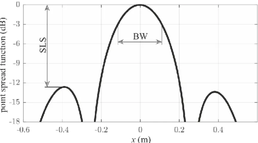
Two criteria, being relevant from the viewpoint of beamforming map quality, were chosen for evaluating he arrays. These are the two properties of the point spread function that are usually investigated: the main lobe beam width BW, and the side lobe suppression SLS. An illustrative point spread function is shown in Fig. 1., where these quantities are shown.
Here the strongest peak is called the main lobe, while the other peaks, resulting from partial coherence, are called side lobes. The width of the main lobe is measured 3 dB down from its maximum strength. This value is related to the resolution of beamforming, i.e. the ability to discriminate between sources being in the close vicinity of each other. The smaller BW, the better the resolution, therefore BW is to be minimised. Another property is the side lobe suppression SLS, which is the beamform level difference of the main lobe and the strongest side lobe. This is important, as it practically limits the dynamic range when visualising and analysing beamforming maps. To increase the useful dynamic range, while avoiding side lobe effects, SLS should be maximised.
3 NUMERICAL PROCEDURE
Numerical case studies were generated and evaluated. Synthetic sources were created using a program previously applied in [7]. This creates the signal vector at equidistant time instants, being five times oversampled compared to the final sampling rate. Then these values are numerically propagated to the microphone positions using a free-field Green function. The arriving signals and the times of flight are computed, and the arrival times are determined.
Finally, using spline interpolation, the arriving signal is interpolated onto the receiver time vector having a pre-defined constant sampling rate. Thus the 𝑝𝑚(𝑡) values “recorded” by the microphones are obtained.
Fig. 1. A point spread function
6
The sampling frequency of the generated signal was set to 51200 Hz, while the length was 1 s. This was found adequate after initial tests, since the beamforming results did not vary after increasing this sample length. The virtual rotating array method is applied to remove the effects of rotation from the 𝑝𝑚(𝑡) signals using the procedure described in Section 2. Then the cross- spectral matrix is constructed from averaging the spectra of the signals using 1024 samples for the Fast Fourier Transform, with von Hann windows and a 50% overlap. About 100 windows are averaged to get a final spectrum. The diagonals are not modified in any way. Then, conventional beamforming was carried out using the steering vector “formulation II” from [8], and its results are reported in decibels by the beamforming level L.
Beamforming was carried out on a grid covering an area of 1 m by 1 m, with 5 mm grid size.
The sources were placed in this plane, being z=1 m away from the array. The array had a diameter of 1 m, was circular in shape, with its centre at point (x, y)=(0, 0), falling onto the axis of revolution.
The beam width BW was evaluated by considering the total number of grid points, whose beamform level was not more than 3 dB below the maximum. Then, using the grid spacing, the area of the main lobe was determined, and the diameter of an equivalent circle, i.e. one that has the same area as the main lobe, was calculated. This diameter was used to characterise the main lobe width. Care was taken to ensure that no side lobes fall into this 3 dB range.
Side lobe suppression (SLS) was determined using the following algorithms. First, local maxima were localised, being those points, where Ln is higher, then at all eight of its neighbours.
Next, the global maximum, where the source is located, was removed from this list. Finally, the local maximum with the largest L value of the remaining points was found, and the SLS was found as the difference of its L value and the main peak L value.
Investigations were carried out at the following frequencies: 2 kHz, 3150 Hz, 4 kHz, 5 kHz, 6300 Hz. These are the mid-frequencies of third-octave bands that are most relevant for the investigation of axial fans [9], as well as having an acceptably low main lobe size. One source was initially located at the origin (x, y)=(0, 0), while the others at radii 0.1 m and 0.2 m, with an angular separation of 45°. Thus 17 positions were investigated in total for each case and each frequency.
4 RESULTS
4.1 Non-uniform microphone arrangements
The proposed generalisation of the VRAM method allows the application of non-uniform microphone arrays for rotating sources. This may be beneficial to reduce the beam width and increase the side lobe suppression. Different microphone arrangements, described by the
7
microphone angular locations 𝛾𝑚 are proposed. They are described by power functions, being characterised by a single exponent d>0, in the following way:
𝛾𝑚 = 2𝜋 (𝑚 − 1 𝑀 )
𝑑
. (10)
This approach was chosen, since it guarantees that 𝛾𝑚 are monotonous, is easy to handle, contains only one parameter, therefore easy to optimise, and reduces to the equidistant array at d=1. In case of 𝑑 ≤ 0.5, the PSF became so smeared that interpreting the results was difficult, while similar problem occurred at d>1.5. This meant that the side lobe suppression was less, than 3 dB, therefore the beam width could not be calculated reliable. These cases were not evaluated, as they such a low SLS value is probably not useful in a real situation. Due to this, the range d=0.6, … 1.5 was investigated in steps of 0.1. Figure 2 shows some arrays obtained with different d values.
The rotation speed n had very little observable effects on the point spread function, therefore this was not investigated any further in the present study. The results are of n=20 1/s.
Figure 3. shows the beam width BW normalised by the wavelength 𝜆 with varying d in the aforementioned range. This figure shows the results of all 17 positions and all 6 frequencies:
the circles indicate the mean, while the error bars show the minima and the maxima. The average beam width is lowest at d=1, corresponding to the equidistant array. The range of the normalised beam widths is lowest there, as well, indicating that this may be the optimum choice for an array. The region around d=1 was investigated in detail, by decreasing the step size in d, but d=1 was found the be the best choice, guaranteeing the smallest main lobe beam width there, as well. It should be noted however, that in some configurations, it is possible to reach significantly smaller main lobes, than the average at d=1.
The side lobe suppression SLS is shown in Fig. 4 against the exponent d. Similarly to Fig.
3, both the range and the mean are indicated by circles and error bars, respectively. In this case the d=1 case performs best again, having the highest SLS value of the investigated setup. The range of the SLS values approximately agrees throughout the investigated domain.
Based on these findings, we can conclude that a power law arrangement is not beneficial for the design for circular microphone arrays, as it performs no better than a simple equidistant array. Similar investigations were carried out with a logarithmic law array as well, where the arrangement closest to linear was found best, but its results were worse than those of the uniform linear array.
8
Fig. 2. Some power law arrangements.
9
Fig. 3. Normalised beamwidth against the power law exponent. Circles: average of all frequencies and all source locations. Error bars: maxima and minima.
Fig. 4. Side lobe suppression against the power law exponent. Circles: average of all frequencies and all source locations. Error bars: maxima and minima.
10
4.2 Sensitivity of the original VRAM to angular errors
In this section, the effect of microphone angular placement errors on beamforming output are investigated. The scenario is the following. One may intend to build an equidistant circular array, however, manufacturing errors and tolerances may cause different angular separations.
By measuring the true microphone locations, this can be corrected in terms of the weight vectors, however, when the original VRAM formulation is used, some inaccuracies will arise.
The magnitude of these effects is investigated in this section, by starting with an equidistant microphone array, and then gradually modifying the position of one selected microphone. The simulated noise is processed by VRAM to get an estimate for the flawed measurement, while the extended VRAM method is used to get a correct result. For both cases, weight vectors corresponding to the actual microphone locations are used. The results of the two algorithms are compared in terms of maximum peak level, beam width and side lobe suppression, to see the effects of the angular error.
For this investigation, the 17 source locations, noted previously, were used. The data showed significant variation depending on source position, therefore this is important to consider.
Different rotation speeds were tested as well, but their effect was found to be small, therefore n=20 1/s was used. The third-octave band centre frequencies of 2 kHz and 6.3 kHz were tested, and it was concluded that higher f leads to higher discrepancies in the data. This is understandable as the interpolation was expected to perform worse for smaller wavelengths, if the position error is constant. In the present case of M=32 microphones, the angular separation between them is 11.25°. The 𝛿𝛾 angular errors between 0° and 10° were tested in steps of 2.5°.
The position of the 10th microphone was modified by this value: 𝛾′10= 𝛾10+ 𝛿𝛾. Simulations were carried out using this setup for each location.
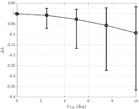
Figure 5. shows how the maximum of the beamforming level changes as the angular error increases. Similarly to the previous figures, the circles indicate the mean, while the error bars show the range. As expected, the difference of the maxima has a decreasing tendency. This means that as the position error of the microphone increases, applying the VRAM method introduces some imprecisions into the computation, which will decrease the coherence at the beamforming step. At 0° angle error, obviously, no such effect can be observed, but as the angle increases, the maximum beamform level will decrease faster and faster. The effect is however very small, as even a 10° error will only cause the loss of about 0.1 dB, which is usually negligible in case of real-world beamforming experiments. Furthermore, this is already an extreme angular inaccuracy that was included only as guidance. For lower angles, possibly resulting from manufacturing imprecisions, this effect is negligible.
11
The effect of this angle error was studied on the beam width and the side lobe suppression of the results, as well. In case of beam width, no significant effect can be observed. The side lobe suppression worsened, following an approximately linear function with respect to the angular error, however, this was also a small effect, being about 0.1 dB at 𝛿𝛾10 = 10°.
5 SUMMARY
An extension of the virtual rotating array method was proposed that enables the application of arrays with uneven microphone placements. The main motivation was to increase side lobe suppression and reduce main lobe beam width by selecting appropriate microphone arrangements, following the approach usual for conventional beamforming. After some preliminary tests with synthetic sources, using a power law arrangement, we can conclude that these distributions are not beneficial. From the points of view of both side lobe suppression and main lobe beam width, the uniformly distributed linear array performed best. This means that a power law is not suitable for arranging circular microphone arrays.
The sensitivity of the original VRAM method with regards to microphone angular placement error, due to manufacturing uncertainty, was investigated as well, by comparing the results of the original and the extended method for arrays with uneven microphone distribution. The data show that the results of angular imprecision is quite small in case of an array with M=32 microphones, as only about 0.1 dB difference was observed due to the imperfect array when
Fig. 5. Change of maximum beamforming level as a function of angle error
12
the angle was 10°. This would be larger for an array with less microphones, however, would probably still be negligible in any practical array setup.
In the future, a detailed optimisation procedure is planned, to see whether a better circular array can be designed by using different distributions or genetic algorithms. It is suggested to arrange the microphones along more, concentric circles [3]. Investigating this setup would be a useful approach, as well, where better results could probably be achieved. Besides that, we aim to show analytically for conventional beamforming, that the equidistant array is truly an optimum. These will lead to better understanding of circular arrays, being important for the analysis of rotating sound sources.
ACKNOWLEDGEMENTS
This work has been supported by the Hungarian National Research, Development and Innovation Centre under contract No. K 112277.
On behalf of Bence Tóth, the project is supported by the ÚNKP-16-3-I. New National Excellence Program of the Ministry of Human Capacities.
The work relates to the scientific programs “Development of quality-oriented and harmonized R+D+I strategy and the functional model at BME” (Project ID: TÁMOP-4.2.1/B- 09/1/KMR-2010-0002) and “Talent care and cultivation in the scientific workshops of BME”
(Project ID: TÁMOP-4.2.2/B-10/1-2010-0009).
REFERENCES
[1] R. P. Dougherty. “Beamforming in acoustic testing.” In Experimental Aeroacoustics, T.
J. Mueller, (ed). Berlin, Springer, 2002.
[2] B. E. Walker and R. P. Dougherty. “Virtual Rotating Microphone Imaging of Broadband Fan Noise.” AIAA-2009-3121, 2009. 15th AIAA/CEAS Aeroacoustics Conference, Miami, Florida, 11-13 May 2009.
[3] G. Herold and E. Sarradj. “Microphone array method for the characterization of rotating sound sources in axial fans." Noise Control Engineering Journal, 63 (6), 546–551, 2015.
[4] P. Sijtsma, S. Oerlemans, and H. Holthusen. “Location of rotating sources by phased array measurements.” AIAA-2001-2167, 2001. 7th AIAA/CEAS Aeroacoustics Conference, Maastricht, 1–13 March 2001.
[5] F. J. Zenger, G. Herold, S. Becker, and E. Sarradj. “Sound source localization on an axial fan at different operating points.” Experiments in Fluids, 57 (8), 136, 2016.
[6] J. R. Underbrink. “Aeroacoustic Phased Array Testing in Low Speed Wind Tunnels.” In Experimental Aeroacoustics. T. J. Mueller, (ed). Berlin, Springer, 2002.
13
[7] Cs. Horváth, B. Tóth, P. Tóth, T. Benedek, and J. Vad. “Reevaluating noise sources appearing on the axis for beamform maps of rotating sources.” FAN 2015 - International Conference on Fan Noise, Technology and Numerical Methods, Lyon, 15-17 April 2015.
[8] E. Sarradj. “Three-dimensional acoustic source mapping with different beamforming steering vector formulations.” Advances in Acoustic and Vibration, 2012, ID: 292695.
[9] T. Benedek and J. Vad. “An industrial onsite methodology for combined acoustic- aerodynamic diagnostics of axial fans, involving the phased array microphone technique.” International Journal of Aeroacoustics, 15 (1-2), 81–102, 2016.