THE MOTION AND SPIN EVOLUTION OF EXTENDED BODIES IN ROTATING BLACK HOLE SPACETIMES

(1)

ZOLT ÁN KERESZTES¹, BAL ÁZS MIK ÓCZI²

1Department of Theoretical Physics, University of Szeged, Tisza Lajos krt 84-86, 6720 Szeged, Hungary

Email: zkeresztes@titan.physx.u-szeged.hu

2Research Institute for Particle and Nuclear Physics, Wigner RCP, H-1525 Budapest 114, P.O. Box 49, Hungary

Abstract. We investigate the evolution of spinning bodies moving along unbound orbits in different rotating (singular/regular) black hole spacetimes. The evolutions describe such scattering processes during which the bodies enter the ergosphere of the rotating black holes but remain outside of the outer event horizon. The considered orbits run close to the equatorial plane. We illustrate the spin influences on the orbit dynamics and that the spin precessional angular velocity is highly increased near and within the ergosphere. The scattering processes are characterized by the final values of spin and orbital plane orientation angles and azimuthal Boyer-Lindquist coordinate.

Their dependencies on the initial spin angles and a characteristic black hole parameter are discussed.

Key words: General Relativity – Gravitation – Black hole – Celestial Mechanics.

1. INTRODUCTION

In the general relativity in both presence and absence of standard model matter fields any black hole solution contains a spacetime singularity where the validity of the theory breaks. However in the presence of non-standard matter fields, singularity free spacetime solutions describing black holes can be obtained. In the recent years, these regular black holes have been widely studied, see for example Refs. Bianchi et al.(2015); Toshmatovet al.(2015); Abdujabbarovet al.(2016); Maluf and Neves (2018); Toshmatovet al.(2019).

The first metric characterizing a spacetime of a non-rotating regular black hole was proposed by Bardeen (Bardeen, 1968). This metric was interpreted as describing the spacetime surrounding a magnetic monopole which occurs in a nonlinear electrodynamics (Ay´on-Beato and Garc´ıa, 2000). The nonlinear electrodynamics is constructed in terms of an antisymmetric electromagnetic field tensor as the Maxwell theory but the Lagrangian is modified. A nonrotating regular black hole spacetime was also proposed by Hayward (Hayward, 2006) having similar interpretation with another Lagrangian for the nonlinear electrodynamics (Fan and Wang, 2016). A more generic metric containing the subcases suggested by Bardeen and Hayward, and in-

Romanian Astron. J. , Vol.30, No. 1, p. 61–81, Bucharest, 2020

(2)

cluding the rotation of the black hole was derived in Ref. Toshmatovet al.(2017a), which we will consider in this paper.

In order to discover the distinguishability of singular and regular black hole spacetimes we consider the evolution of extended^∗ spinning bodies moving along unbound orbits. Note that hyperbolic orbits of spinning bodies about singular black holes in the extreme mass ratio limit were already investigated by using the Matthison- Papapetrou-Dixon (MPD) equations (Biniet al., 2017a). Analytic computations in Ref. Biniet al.(2017a) were carried out for small spin magnitudes whose direction is parallel to the central black hole rotation axis and when the body moves in the equatorial plane. In this configuration the spin direction is conserved. In our investigation the spin axis is not parallel to the black hole rotation axis. As a consequence, the orbit of the body is not confined precisely to the equatorial plane and the spin direction evolves. In addition the closest approach distance during the evolution is inside the ergosphere where a post-Newtonian approximation fails. Therefore we use the MPD equations for description of the evolution.

The paper is organized as follow. In Section 2 we introduce the MPD equations, the metric characterizing the spacetime of the considered rotating, singular/regular black holes, and two fundamental families of observers, the static and the zero angular momentum ones. We set two frames of co-moving observers by boosting the static and the zero angular momentum observers’ frames and describe the spin evolution in them. In Section 3 the discussion of scattering processes based on numerical simulations are presented while Section 4 contains the conclusions.

2. THE DYNAMICS OF THE EXTENDED BODIES IN ROTATING, REGULAR BLACK HOLE SPACETIMES

2.1. EVOLUTION EQUATIONS

The MPD equations (Mathisson, 1937; Papapetrou, 1951; Dixon, 1970, 1976) describe the motion of an extended spinning body in curved spacetime in the pole- dipole approximation, which read as

Dp^a

dτ = −1

2R^a_bcdu^bS^cd, (1) DS^ab

dτ = p^au^b−u^ap^b. (2)

∗An extended body is described by an infinite series of multipole moments (Dixon, 1964). A point- like particle only has the monopole moment. The body in the Matthison-Papapetrou-Dixon model (used in this paper) is described in the pole-dipole approximation when it is characterized by mass and spin, with all the higher multipoles neglected.

(3)

HereD/dτ=u^c∇cis the covariant derivative along the integral curve of the four ve- locityuâobeying the normalizationuâua=−1,Râ_bcd is the Riemann tensor of the background spacetime, andpâ andSâb are the four-momentum and the spin tensor of the moving body, respectively. The MPD equations are closed with a spin supple- mentary condition (SSC) which determines the representative point for the extended body. In this paper we use the Tulczyjew-Dixon (TD) SSC (Tulczyjew, 1959; Dixon, 1970) imposingp_aSâb= 0. This SSC together with the MPD equations results in two constants of motion: the spin magnitudeS=p

S_cdS^cd/2 and the dynamical mass M =√

−p^ap_a. The TD SSC and the MPD equations yield the following velocity- momentum relation (Semer´ak, 1999):

u^b= m M²

p^b+ 2S^baR_aecdp^eS^cd 4M²+R_aecdS^aeS^cd

, (3)

where m=−u_ap^a is the mass measured in the rest frame of the observer moving with velocityu^a.

In addition, we introduce a spin four vector as S^a=− 1

2Mη^abcdp_bS_cd, (4)

whereη_abcd is the 4-dimensional Levi-Civita tensor which is totally antisymmetric andη₀₁₂₃=√

−g, wheregis the determinant of the metric.

2.2. ROTATING, REGULAR BLACK HOLES

The considered line element squared in Boyer-Lindquist coordinates (t, r, θ, φ) (Toshmatovet al., 2017a)^†is given by

ds² = −∆−a²sin²θ

Σ dt²−2aBsin²θ Σ dtdφ +Σ

∆dr²+Σdθ²+A

Σsin²θdφ², (5) whereais the rotation parameter,

Σ=r²+a²cos²θ, (6)

∆=r²+a²−2α(r)r , (7) B=r²+a²−∆, (8)

†There are discussions (Bronnikov, 2017; Rodrigues and Junior, 2017; Toshmatovet al., 2017b) on that the rotating regular black hole spacetime presented in Ref. Toshmatovet al.(2017a) is not an exact solution of the field equations. However it is proved that the presented spacetime may differ only per- turbatively from the exact solution (Toshmatovet al., 2017b), therefore it is suitable for consideration of spinning bodies evolutions.

(4)

and

A= r²+a²2

−∆a²sin²θ. (9) The functionα(r)is

α(r) =µ+ µ_emr^γ

(r^ν+q^ν_m)^γ/ν . (10) For a vacuum spacetimeµ_em= 0, andµrepresents the mass parameter of the black hole. In this case (5) reduces to the Kerr metric (Kerr, 1963). When a nonlinear electrodynamic field is present in the spacetime,µ_em=q³_m/σ6= 0is interpreted as an electromagnetically induced ADM mass (Toshmatovet al., 2018). The quantity σ in the expression of µ_em controls the strength of the nonlinear electrodynamic field and carries the dimension of length squared whileq_m is related to the magnetic charge (Fan and Wang, 2016). The spacetime is free from the singularity forµ= 0 andγ≥3. In the case ofµ= 0 and µ_em6= 0, the powers (γ,ν) are (3,2) for the Bardeen and (3,3) for the Hayward subcases (Toshmatovet al., 2017a).

The stationary limit surfaces and the event horizons (if they exist) are determined by the solutions of gtt= 0 andg^rr= 0, respectively. The region which is located outside the outer event horizon but inside the outer stationary limit surface is called ergosphere. The existence of the stationary limit surfaces and the event horizons are strongly dependent on the parameter qm, see Figs. 3 and 4 in Ref.

Toshmatovet al.(2017a). For the chosen parameter values in the next section, the regular black holes will have similar structure like the Kerr spacetime,i.e.they have two event horizons and two stationary limit surfaces and the spacetime contains an ergosphere in all cases.

In the following we introduce two family of observers. The frame of the static observers (SOs) is given by the tetrad

e0 = 1

√−g_tt∂r, e1= r∆

Σ∂r, e2= ∂θ

√Σ , e3 = − 1

√∆

aBsinθ Σ√

−g_tt∂_t−

√−g_tt sinθ ∂φ

, (11)

while that of the zero angular momentum observers (ZAMOs) by f0 =

r A Σ∆

∂_t+aB A∂φ

, f1=

r∆ Σ∂_r, f2 = ∂θ

√Σ, f3= rΣ

A

∂φ

sinθ . (12)

Following Ref. Bini et al. (2017b), we define Cartesian-like 3-bases (ex, ey, ez) and(fx, fy, fz) in the local rest spaces of the SOs and the ZAMOs by (e1, e2, e3)

(5)

= (e_x, e_y, e_z)R(θ,φ)and(f₁, f₂, f₃) = (f_x, f_y, f_z)R(θ,φ), respectively, where R(θ,φ) =





sinθcosφ cosθcosφ −sinφ sinθsinφ cosθsinφ cosφ

cosθ −sinθ 0



 (13) is the same rotation matrix which locally relates the unit basis vectors of Cartesian and spherical coordinates in the 3-dimensional Euclidean space. The orbit of the spinning body will be represented in the coordinate space

x = rcosφsinθ, y = rsinφsinθ,

z = rcosθ. (14)

We characterize the instantaneous plane of the motion in the (x,y,z)-space by the unit vector:

l= R×V

|R×V| , (15)

where × is the cross product in Euclidean 3-space, R is the position vector with components:

R^x=x , R^y=y , R^z=z , (16) andVis a spatial velocity vector with^‡

V^x=dx

dτ , V^y=dy

dτ , V^z=dz

dτ. (17)

The absolute value in the denominator denotes the “Euclidean length” of the numera- tor. Since the considered spacetimes are asymptotically flat, the quantitylⁱcoincides with the direction of the orbital angular momentum^§at the spatial infinity.

We describe the spin dynamics in the comoving frame obtained by boost trans- formations from the frames of the static and zero angular momentum observers.

When boosting the static observer’s frame we obtain the co-moving frame as E0(u) =u , Eα(e, u) =eα+ u·e_α

1 +Γ_(S) u+u_(SO)

, (18)

‡Noting that we could use any timelike parameter in the definition (17) due to the normalisation in Eq. (15).

§We mention that the natural definition of orbital angular momentum aboutx₀would be L^ab=−σ^[a(x, x0)p^b](τ).

Here σ^a is a generalized position vector which can be computed from the Synge’s world function (Synge, 1960). However there are only few metrics for which the exact world function is known (Ruse, 1930; Gunther, 1965; Buchdahl, 1972; Buchdahl and Warner, 1980; John, 1984, 1989; Roberts, 1993).

(6)

withu_(SO)=e₀,Γ_(S)=−u·u_(SO)andα={1,2,3}, while boosting the zero angular momentum observer’s frame we have

E0(u) =u , Eα(f, u) =fα+ u·fα

1 +Γ_(Z) u+u_{(ZAM O)}

, (19)

withu_{(ZAM O)}= f₀andΓ_(Z)=−u·u_{(ZAM O)}. Here the dot denotes the inner product with respect to the background spacetime metric. A spatial rotation about the axis n^αwith non-vanishing components

n¹=− w₍²Z)

r

w¹_(Z)2

+

w²_(Z)2 and n²= w₍¹S)

r

w_(S)¹ 2

+

w_(S)² 2 (20) by an angleΘdetermined from

sinΘ=−

"

1− s

Σ∆

−g_ttA

!Γ_(S)w_(S)³

1 +Γ_(S) − aBsinθ

√−g_ttΣA

#Γ_(S) r

w¹_(S)2

+ w_(S)² 2

1 +Γ_(Z) , (21) transforms the frame vectorsEA(e, u)toEA(f, u)(whereA={0,1,2,3}). Here w_(S)=Γ_(S)⁻¹u_(SO)−uandw_(Z)=Γ_(Z)⁻¹u_{(ZAM O)}−uare the relative spatial velocities of the SO and ZAMO, respectively, with respect to the moving body in the co-moving frame.

When boosting the Cartesian-like SO and ZAMO frames we obtain the respec- tive co-moving Cartesian-like frames which are also spatially rotated with respect to each other. The spin evolution in the co-moving Cartesian frame is described by the precession angle velocity:

Ω^β_(prec)=−Ω^β_(orb)+Ω^β, (22)

where Ω^β_(orb) is given by Eq. (87) of Ref. (Bini et al., 2017b), and Ω¹ =E₃· DE₂/dτ, Ω²=−E₃·DE₁/dτ andΩ³ =E₂·DE₁/dτ(Biniet al., 2017b). The Ω^β_(prec)(e, u)andΩ^β_(prec)(f, u)denote precession angle velocities in the boosted SO and ZAMO co-moving Cartesian frames, respectively.

3. NUMERICAL INVESTIGATION

We consider the evolution of spinning bodies following unbound orbits. During the evolution the bodies cross through the ergosphere of the rotating black holes at the closest approach. Regarding the rotating black hole we investigate three cases:i) Kerr black hole (µ6= 0andµ_em= 0);ii)rotating Hayward regular black hole (µ= 0, µ_em6= 0,γ= 3andν= 3); and rotating Bardeen regular black hole (µ= 0,µ_em6= 0,

(7)

γ= 3andν= 2). The rotation parameter is chosen asa= 0.99˜µwithµ˜=µfor Kerr spacetime and˜µ=µ_emfor regular black holes.

For the numerical investigation the initial position of the body is chosen as θ(0) =π/2, r(0) = 2000˜µ,φ(0) = 0 =t(0) , (23) and the independent components of the initial four momentum as

p^r(0)/M =−0.9,µp˜ ^φ(0)/M = 8×10⁻⁷, µp˜ ^θ(0)/M = 0. (24) With these initial values we guarantee that the body will remain in the equatorial plane if it has no spin or its spin axis is aligned or anti-aligned with the rotation axis of the central black hole. In addition the initial spin vector of the body is characterized in the comoving Cartesian frame set up by boosting the SO frame. Then

S=SⁱE_i(e, u) , (25)

wherei={x,y,z}and Sⁱ=|S|

cosφ^(S)sinθ^(S),sinφ^(S)sinθ^(S),cosθ^(S)

. (26)

The angles θ^(S) and φ^(S) are the spherical polar angles of the spin vector in the comoving Cartesian frame. The validity of the MPD dynamics requires the spin magnitude|S|/˜µMto be small which is chosen as|S|/˜µM= 0.01(Hartl, 2003).

We note that in case of Kerr spacetime, with a corresponding rescaling of coordinates and introducing dimensionless variables the parametersµ andM can be eliminated from the numeric consideration. Similarly, following Ref. Toshmatovet al.(2017a) for regular black holes, it can be achieved that only the combination

q= qm

µ_em , (27)

enters explicitly in the numeric equations given in terms of dimensionless variables.

The spacetime is only regular for q 6= 0while the limit q →0 results in the Kerr spacetime with mass parameterµ=µ_em(Toshmatovet al., 2017a). For the regular Bardeen (ν= 2) and Hayward (ν= 3) subcases there is a black hole in the spacetime forq≤0.081andq≤0.216, respectively. The event horizon disappears for higher values ofq.

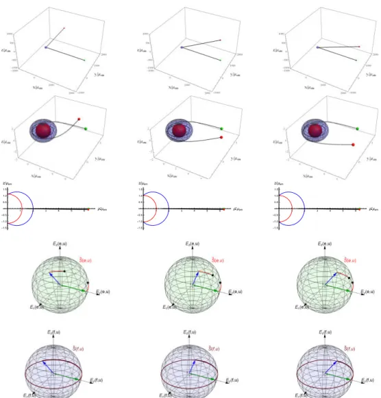
On Fig. 1 the evolutions of spinning bodies in different spacetimes are shown.

The initial spin angles are chosen asφ^(S)(0) =π/2andθ^(S)(0) =π/2. The three columns represent the following parameter choices for the background spacetime:

rotating Hayward black hole withq= 0.081(left column) and withq= 0.216(mid- dle column) and rotating Bardeen black hole with q= 0.081(right column). The evolution in a Kerr spacetime with mass parameterµ=µ_emis barely distinguishable from the case presented in the left column, therefore it is not shown separately. The first row depicts the unbound orbits in the (x,y,z)-space. The initial and the final

(8)

positions of the body are marked by green and red dots, respectively. The second and third rows represent the same orbit in the near region of the black hole in the (x,y,z) and the (ρ=rsinθ,z=rcosθ) coordinate spaces. In the second row the red and the blue surfaces at the centre depict the inner (the outer event horizon) and outer (the outer stationary limit surface) bounds of the black hole’s ergosphere, respectively.

In the third row the inner and outer bounds of the ergosphere are indicated by red and blue curves. As the body enters in the ergosphere it makes two turns about the black hole, then it leaves the ergosphere going to the spatial infinity. The fourth and fifth rows image the spin vector represented in the boosted SO and ZAMO Carte- sian frames, respectively. Since SOs only exist outside of the ergosphere, the spin evolution cannot be represented in the boosted SO frame when the body stays in that region. The jump in the evolution of the spin vector in the boosted SO frame (marked by black dots) emphasizes that a relatively large part of the variation in the spin direction takes place inside the ergosphere.

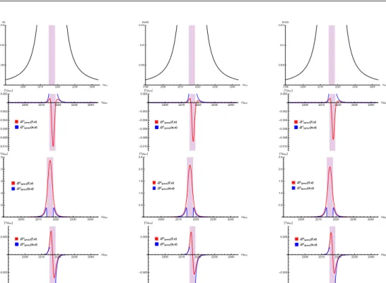
On Fig. 2, we show the evolutions of the rotation angleΘdefined by Eq. (21) (first row) and the spherical co-moving triad components of the precessional angular velocitiesΩ^α_(prec)(e, u)andΩ^α_(prec)(f, u)when the body is close to the central black hole. The purplish shadow represent that period where the body is inside the ergosphere. The angleΘ is small when the body is relatively far from the central black hole. Where this angle is small both boosted frames (SO and ZAMO) can be equally used for description of the spin dynamics. The blue lines representing the precessional velocity triad components in the boosted SO frame diverge at the location of the outer stationary surface. This is because SOs only exist outside of the ergosphere, thus the boosted SO frame cannot be used for description of the spin evolution at that location. However the boosted ZAMO frame can be used and the red curves show that the spin precessional velocities are highly increased within the ergosphere.

The increased spin precession near the ergosphere can be supported without using a particular frame. Fig. 3 shows the Boyer-Lindquist coordinate components of the unit spin vectorS^a/Sand their derivatives in case of a central rotating Hayward regular black hole with q= 0.216. The first and the second rows show the evolution of the Boyer-Lindquist coordinate components of the unit spin vector and their derivatives on the total considered timescale, respectively. While the third row represents these evolutions in that period where the body is close to the central black hole.

The panels show that the unit spin vector coordinate components and their derivatives undergo significant changes when the body is near and inside the ergosphere.

In the forthcoming we investigate the variation of the final spin and orbital plane orientation (given by Eq. (15)) angles as functions of initial spin angles and the black hole parameterq. The polar and azimuthal angles of the instantaneous orbital plane orientation will be denoted byθ^(l)andφ^(l), respectively. Forτ>τ^∗= 4500˜µ, the angles θ^(l), φ^(l), θ^(S) and φ^(S) undergo only unsignificant changes, thus we

(9)

characterize the scattering process with their values atτ^∗.

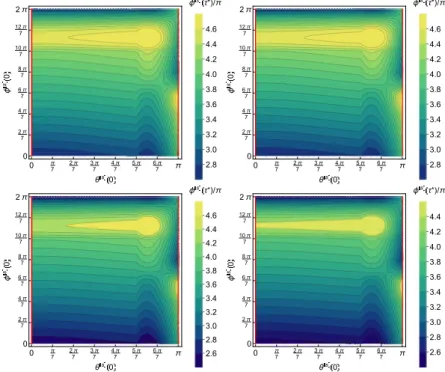
The polar anglesθ^(s)(τ^∗)andθ^(l)(τ^∗) are shown on Fig. 3 in the parameter space of initial spin angles θ^(s)(0) and φ^(s)(0). These color maps are independent from the chosen background spacetime (Kerr, Hayward or Bardeen). The left panel expresses thatθ^(s)(τ)is almost a constant. The right panel shows thatθ^(l)(τ) also undergoes only a small variation which is the largest for the initial spin angles θ^(s)(0)≈3π/7...4π/7.

On Figs. 5 and 3 we present the azimuthal anglesφ^(s)(τ^∗)andφ^(l)(τ^∗)in the parameter space of

θ^(s)(0),φ^(s)(0)

, respectively. From top left to bottom right the background spacetimes are Kerr, rotating Hayward withq= 0.081, rotating Hayward withq= 0.216and rotating Bardeen withq= 0.081. The red lines on both sides represent the cases when the azimuthal anglesφ^(s)andφ^(l)are indefinite because then the spin is parallel/anti-parallel with the rotation axis of the central black hole during the whole evolution and the body remains in the equatorial plane. For another initial values the spin is precessing and we show the cumulative value ofφ^(s). However for the azimuthal angle of the orbital orientation we present φ˜^(l)(τ^∗) =φ^(l)(τ^∗) mod 2π. This is because θ^(l)(τ) vanishes multiple times and then φ^(l) becomes undetermined. On both figures the panels in the first lines share more similari- ties. The local maxima of φ^(s) are in the following

θ^(s)(0),φ^(s)(0)

domains [5π/7..6π/7,10π/7..12π/7]and[9π/10..π,5π/7..6π/7]on all panels. These local maxima are decreasing from top left to bottom right. The maximum ofφ^(l)is in the domain[5π/7..6π/7,12π/7..2π]for the first two panel while in[2π/7..3π/7,0..2π/7]

for the third one and[5π/7..6π/7,0..2π/7]for the fourth panel.

In the considered cases the orbit of the spinning body is confined close to the equatorial panel. Therefore the value of the Boyer-Lindquist coordinate φatτ^∗ is also good parameter for the characterization of the scattering process. Its value in the parameter space of

θ^(s)(0),φ^(s)(0)

is presented on Fig. 7. The picture shows that φ(τ^∗)is independent fromφ^(s)(0)while it is an increasing function ofθ^(s)(0).

The Figs. 5, 3 and 7 proves that the valuesφ^(s)(τ^∗),φ˜^(l)(τ^∗)andφ(τ^∗)depend on the parameters of the background spacetime and the most significant changes occurs inφ(τ^∗).

On Fig. 3 and 9 we present the dependence of the final values of spin angles and orbital plane orientation angles, respectively, on the parametersqandφ^(s)(0)in rotating Hayward (left column) and Bardeen (right column) spacetimes, remember- ing thatq→0corresponds to the Kerr limit. For these figures the initial polar spin angle is chosen asθ^(s)(0)≈π/2. Interestingly the color maps on the left and right hand sides are similar to each other but it must be emphasized that the ranges of q are very different. Apart from some relatively small domains, we find higher values for the considered angles at fixedqin case of rotating Hayward background.

(10)

Table 1

The coefficientsα,h,δandωof the shifted sine function at differentqvalues in case of a central rotating Hayward black hole, see Fig. 11

q α h δ ω

0 −0.1109 4.5542 1.5361 0.9998 0.031 −0.1108 4.5533 1.5361 0.9998 0.062 −0.1101 4.5467 1.5364 0.9998 0.093 −0.1081 4.5292 1.5371 0.9998 0.123 −0.1044 4.4960 1.5384 0.9998 0.154 −0.0988 4.4440 1.5403 0.9999 0.185 −0.0915 4.3720 1.5429 1.0000 0.216 −0.0829 4.2810 1.5460 1.0001

Table 2

The coefficientsα,h,δandωof the shifted sine function at differentqvalues in case of a central rotating Bardeen black hole, see Fig. 11

q α h δ ω

0 −0.1109 4.5542 1.5361 0.9998 0.012 −0.1100 4.5451 1.5364 0.9998 0.023 −0.1071 4.5182 1.5373 0.9998 0.035 −0.1027 4.4752 1.5388 0.9998 0.046 −0.0970 4.4181 1.5406 0.9999 0.058 −0.0907 4.3498 1.5427 1.0000 0.069 −0.0839 4.2729 1.5450 1.0000 0.081 −0.0771 4.1900 1.5473 1.0001

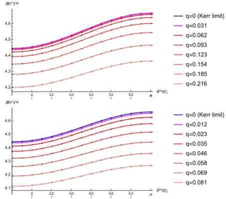
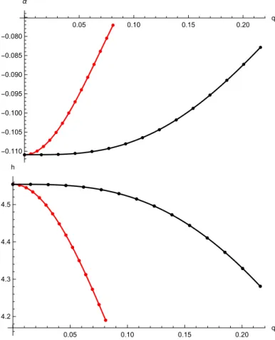
Sinceφ(τ^∗)does not depend onφ^(s)(0)we depict it on Fig. 10 as a function ofqandθ^(s)(0)with a fixed value ofφ^(s)(0) = 0. It turns out that the dependence ofφ(τ^∗) on θ^(s)(0) at fixedq can be described by a simple shifted sine function which is shown on Fig. 11 for rotating Hayward (top panel) and Bardeen (bottom panel) black holes. The values denoted by the dots are determined numerically and the functionαsin

ωθ^(s)(0) +δ

+his fitted at differentq values. The best fitting parameters are shown in Tables 3 and 3 for rotating Hayward and Bardeen regular black holes, respectively. The q = 0 corresponds to the Kerr black hole. These tables show that only the parameters α and h depend on q. The functions α(q) andh(q) are presented on Fig. 12. These functions are very different for rotating Hayward and Bardeen black holes. The parameters of the fitted quartic polynomials aq⁴+bq³+cq²+dare listed in Table 3.

(11)

Table3 Thecoefficientsa,b,canddcharacterizingthefunctions α(q)andh(q)forrotatingHaywardandBardeenblackholes aq4+bq3+cq2+dabcd α(q)forHayward−11.3325.697−0.101−0.111 α(q)forBardeen−80.901−27.2437.899−0.111 h(q)forHayward65.935−44.3680.6514.554 h(q)forBardeen874.359120.081−70.9794.554

(12)

1 2 3 4 5 6 ρ μem

-1.5 -1.0 -0.5 0.5 1.0 1.5 z/μem

1 2 3 4 5 6 ρ μem

-1.5 -1.0 -0.5 0.5 1.0 1.5 z/μem

1 2 3 4 5 6 ρ μem

-1.5 -1.0 -0.5 0.5 1.0 1.5 z/μem

]

Fig. 1 – The evolutions along unbound orbits. The parameter pair (ν,q) characterizing the central regular black hole changes from left to right as (3,0.081), (3,0.216) and (2,0.081). The rows represent

the following: 1st the orbit in the coordinate space (x,y,z), 2nd and 3rd a part of the orbit near the ergosphere in the coordinate spaces (x,y,z) and (ρ,z), respectively, 4th and 5th the unit spin vector in

the boosted SO and ZAMO co-moving Cartesian-like frames, respectively. The outer event horizon and the outer stationary surface on the first three rows are depicted by red and blue colors, respectively.

(13)

2200 2210 2220 2230 2240 τ✴μem 0.005

0.01 0.015 Sin

2190 2200 2210 2220 2230 2240

τ✴μem 0.005

0.01 0.015 Sin✭Θ)

2190 2200 2210 2220 2230 2240

τ✴μem 0.005

0.01 0.015 Sin✭Θ)

Ω¹(prec)(f,u) Ω¹(prec)(e,u)