1
INVESTIGATING THE ROSI AND THE VRA ALGORITHMS REGARDING THEIR CAPABILITY IN LOCALIZING
ROTATING COHERENT NOISE SOURCES
Bálint Kocsis and Csaba Horváth
Budapest University of Technology and Economics, Faculty of Mechanical Engineering, Department of Fluid Mechanics
Bertalan Lajos street 4-6, 1111, Budapest, Hungary
ABSTRACT
When sound sources are coherent, identifying their true positions using currently available beamforming methods is widely regarded as a challenging task. Due to the constant phase difference between the individual source signals, the constructive and destructive interference of the propagating sound waves often results in misleading results, however, the size and geometry of the array, and the characteristics of the applied beamforming algorithms all have a fundamental effect on the obtained results. In this article, two beamforming algorithms designed for rotating noise sources, namely the Rotating Source Identifier (ROSI) and the Virtual Rotating Array (VRA) methods are tested, with the help of simulations. A simple test case has been defined and investigated using 48-microphone circular arrays of various diameters from various distances. The article analyses and compares the results, drawing conclusion regarding the capabilities of the various beamforming methods when used to investigate rotating coherent noise sources.
1 INTRODUCTION
In the 20th century, the number of turbomachinery applications has increased immensely, with the aviation industry being one of the main contributors. Aircrafts have introduced many problems at the airports and in the neighboring areas from a noise emission perspective, which has led to stricter regulations and has resulted in manufacturers paying more and more attention to the noise emissions of their products. The noise emission of turbomachinery, propellers in particular, has become a substantial research topic, exposing their noise generation mechanisms and the characteristics of the noise itself. In case of turbomachinery noise, the presence of tonal components is not uncommon.
When wind tunnel measurements or fly-over tests are carried out, the standard method for noise source localization is using microphone arrays for data acquisition and then
2
beamforming for signal processing. This method has some advantages, which makes it a convenient tool [1]. A single, short measurement is enough for determining the source position, and the microphone array can be placed further from the investigated object, enabling non-intrusive measurements. It can be used for not only stationary sound sources, but for moving ones as well, which, combined with its advantages, makes it an obvious choice for noise source localization of turbomachinery applications. However, choosing an appropriate microphone array and beamforming method for a given test case is not an easy task. One can choose from many different array geometries (e.g. linear, circular, logarithmic spiral, or random arrangement of microphones) and many different beamforming algorithms.
In case of rotating sources, such as the propellers of turbomachinery, the source motion needs to be known, and beamforming should be carried out with respect to the changing relative positions of the sources and the microphones. There are various approaches available in the literature on how this can be done. In one approach, the sound field is measured using a microphone array, which can be any array used in generic acoustic measurements. After the measurement, data is processed in the time domain in a way that the covered distance, and hence the propagation time of the waves, is calculated and compensated for in each sampled time instant. The method of Sijtsma et al. [2] and the method of Minck et al. [3] use this approach in their beamforming algorithms. In a second approach, the measured data is processed in the frequency domain. This approach requires a particular microphone array design. After the measurement, data is processed in the frequency domain in a way that the array is virtually moved together with the source, and the signals are recalculated and compensated for accordingly. The methods of Herold et al. [4] and Pannert et al. [5] are constructed using this approach. The theoretical descriptions of the two approaches are presented in the following section.
2 DESCRIPTION OF THE TWO MOTION COMPENSATION APPROACHES FOR ROTATING SOURCE BEAMFORMING
2.1 Description of sound propagation for time domain beamforming
This description of the time domain beamforming for rotating sources follows the same logic as the description of the Rotating Source Identifier (ROSI) algorithm [2,6], which is representative of the time domain methods. If a source, located at 𝝃, emits a sound 𝜎 at time 𝜏, then this sound will be received at location 𝒙 as signal 𝜒 at time 𝑡. The time difference Δ𝑡𝑒 = 𝑡 − 𝜏 is the propagation time that it takes for the sound to get from 𝝃 to 𝒙, hence it depends on the distance between the source and the microphone. When the source moves relative to the microphone, then this distance changes, and Δ𝑡𝑒 is not constant. If the distance decreases, i.e.
when the source moves towards the microphone, the time scale 𝑡 shrinks as compared to 𝜏.
Consequently, the same number of sound waves are heard in a smaller amount of time, which results in a stationary listener hearing the sound at a higher frequency. And if the distance increases, 𝑡 expands and the perceived frequency decreases. This is the well-known phenomenon of the Doppler Effect.
3
Assuming a monopole point source in a stationary medium, the generated sound field 𝑝 can be described by Eq. (1):
1 𝑐2
𝜕2𝑝
𝜕𝑡2 − ∇2𝑝 = 𝜎 𝑡 𝛿 𝒙 − 𝝃 𝑡 (1)
where 𝑐 is the speed of sound. This equation can be solved for 𝑝. The derivation can be found in [7]. For free field conditions, the solution reads:
𝑝 𝒙, 𝑡 = 𝜎 𝜏
𝐹 𝒙, 𝝃 𝜏 , 𝑡, 𝜏 (2)
with
𝐹 𝒙, 𝝃 𝜏 , 𝑡, 𝜏 = 4𝜋{𝑐 𝑡 − 𝜏 +1
𝑐 −𝝃′ 𝜏 ⋅ 𝒙 − 𝝃 𝜏 } (3) 𝑡 = 𝜏 + 𝒙 − 𝝃 𝜏
𝑐 (4)
Equation (2) can be rearranged in order to calculate a 𝜎 value at location 𝝃 at time 𝜏 from a recorded signal 𝜒 at a given microphone. Thus, 𝜎 shows that if the signal 𝜒 was emitted by a source at location 𝝃, then what the emitted sound would be at the source (moving together with the source).
Since Δ𝑡𝑒 = 𝑡 − 𝜏 changes according to the position of the source, 𝜏 will not be equidistant. Therefore the calculated series 𝜎 𝜏 should be interpolated on an equidistant time series before using it for signal processing methods. Then, the source localization can be estimated with the conventional delay-and-sum procedure in the time domain. The power spectra of the points in the region of interest can be calculated by transforming the signals to the frequency domain.
2.2 Description of sound propagation for frequency domain beamforming This description of the frequency domain beamforming for rotating sources is based on the description of the Virtual Rotating Array (VRA) algorithm [4], which is representative of the frequency domain methods. When the sound sources in a given region of interest are stationary, and their emission does not change significantly over the measurement time, then the sound field can be investigated in the frequency domain instead of the time domain. This has vast computational advantages, given that the amplitude of the source signal is not calculated for every sampled time instant, but rather the entire signal can be described using its frequency values. This is what the VRA method aims to take advantage of. In case of circular motion, the VRA method utilizes the rotational symmetry and manipulates the recorded signals in order to make the moving sources stationary. The measurement requires a particular array design: it should be circular and axially aligned with the axis of the rotation.
From the measured signals, virtually rotating signals are created by interpolating between the actual neighboring microphone positions. If the array has 𝑀 microphones distributed equally around the circle, then the angle 𝛼 between two microphones is
𝛼 =2𝜋
𝑀 (5)
4
The measured region is traced by the angle 𝜑 𝑡 , and the indices of the neighboring microphone signals between which to interpolate can be determined as:
𝑚− 𝑡 = 𝑚 +𝜑 𝑡
𝛼 − 1 mod 𝑀 + 1 (6)
𝑚+ 𝑡 = 𝑚 +𝜑 𝑡
𝛼 mod 𝑀 + 1 (7)
with ⌊⋅⌋ denoting the floor function. The weighting factors for the interpolation can be calculated as:
𝑠+ 𝑡 =𝜑 𝑡
𝛼 − 𝜑 𝑡
𝛼 (8)
𝑠− 𝑡 = 1 − 𝑠+(𝑡) (9)
Using the weighting factors, the virtual rotating signals can be interpolated:
𝑝vr ,𝑚 𝑡 = 𝑠−𝑝𝑚−+ 𝑠+𝑝𝑚+ (10) Then, the 𝑝vr signals provide a base for a frequency domain beamforming of choice, depending on the given application.
The VRA method is capable of handling a changing rotational speed, which comes in handy when measuring turbomachinery. On the other hand, in this form of the VRA method, the medium between the sources and the microphones is not virtually rotated together with the array, which introduces a systematic inaccuracy into the results. The noise source localization performance of this method, as well as the performance of the time domain approach, will be tested with the help of simulations in Section 4.
3 DESCRIPTION OF THE SIMULATION TEST CASES
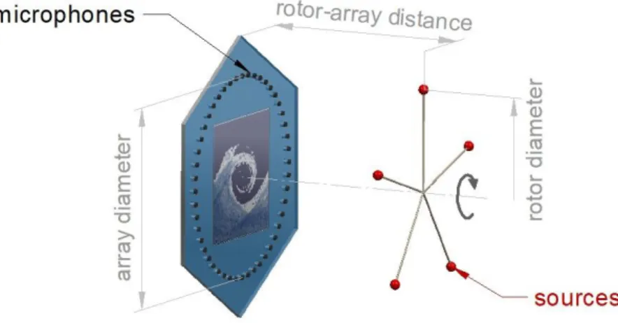
The two beamforming algorithms are tested through simulation test cases. The test cases, illustrated in Fig. 1 consist of a set of rotating monopoles – referred to as the rotor –, and a set
Fig. 1. The arrangement of the rotor and the microphone array.
5
of microphones – referred to as the array. The sources and the microphones are placed on their respective planes, which are parallel and axially aligned. Despite the simplicity of the test case, there are a number of parameters that can be varied: the number of sources, the frequency of the emitted sound, the diameter of the rotor, the angular speed of the rotor, the number of microphones, the diameter of the array, the array geometry, or the distance between the rotor and the array.
3.1 The rotor parameters
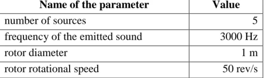
The rotor parameters were fixed throughout the simulations, and are prescribed in Table 1.
Name of the parameter Value
number of sources 5
frequency of the emitted sound 3000 Hz
rotor diameter 1 m
rotor rotational speed 50 rev/s
The rotor parameters are fixed in order to allow the investigation to focus on the array geometry and the beamforming methods applied. However, the effect of changing the source parameters was looked at in a preliminary investigation. Any source number above one results in an interfered sound field in case of coherent sources. Since they are all in phase, adding or taking away one source does not make a significant change in the quality of the results. On the other hand, when the diameter is fixed, and the sources are placed evenly around the circle, the number of sources is important from a resolution point of view. With an increasing number of sources, distinguishing between them becomes harder.
The frequency of the emitted sound was a pure sine wave with a frequency of 3000 𝐻𝑧.
Below 1000 𝐻𝑧 carrying out beamforming on recorded signals becomes problematic, while above 5000 𝐻𝑧 acoustic signals tend to fade out due to the more significant damping. The wavelength, and hence the frequency also affects the acoustic resolution, which improves towards the higher end of the given range. The chosen frequency is somewhere in the middle in both aspects, and can be regarded as a tone of a CROR engine, e.g. the 6th harmonic of a 5- blade at the front, 5-blade at the back, arrangement with 50 𝑟𝑒𝑣/𝑠 rotational speed at both rotors.
The rotor diameter, as mentioned earlier, determines the distance of the sources from one another. Hence it determines the required resolution from the array for the capability to distinguish between the sources. The tangential velocity is determined by the angular velocity combined with the rotor diameter and should be kept well below the speed of sound in order to avoid supersonic effects. With the chosen parameters, the resulting Mach number is approximately 0.46 in the simulation test cases. Preliminary investigations showed that the effect of changing the rotational speed seemed negligible on a wide range, up to a limit that was above the chosen value.
Table 1. The following parameters were always set to the same value throughout the simulations.
6 3.2 The array parameters
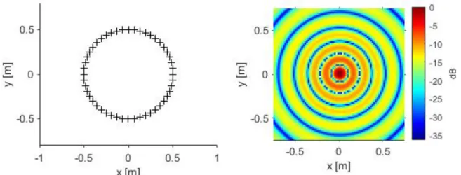
As mentioned in Section 1, the choice of the microphone array (in terms of microphone number and arrangement) is a rather complicated task. However, out of the two algorithms tested here, the VRA algorithm requires a specific geometry, a circle-shaped array, for generating the virtual signals (see the left side of Fig. 2, along with its array pattern on the right) [4]. The same geometry has been used for the ROSI simulations as well in order to avoid a comparison of two different arrays, which is inevitably subjective at some point. It is worth to note, however, that for the latter algorithm, this is not an advantageous array design as the distance between the microphones is the same everywhere. Some improvement might be seen in the performance of the ROSI algorithm if a more suitable array was used.
Therefore, some of the results were compared to other results obtained by using the same parameters but a different microphone arrangement. Although the improvement of the results is not denied, the essential characteristics were preserved when changing to the less-favorable geometry (see an example in Fig. 6).
The circular array consisted of 48 microphones. With an increasing number of microphones, the quality of the beamforming generally improves. This is certainly the case with the VRA algorithm, where the decreasing distance of the microphones improves the quality of the interpolation and hence the virtual signals. It was found by the authors, relying purely on simulation data, that 48 microphones provide proper results in case of the VRA algorithm. This is more than what Herold et al. used when introducing the method [4], but less than what has been used in other simulations [8]. On the other hand, the results of the ROSI algorithm seemed uninfluenced by the addition of more microphones in case of a circular array, as only the computational time increased significantly.
There are two other parameters of the array which are investigated here, the array diameter, and the distance between the rotor and the array. These parameters are closely related to the question of spatial resolution, which is discussed in the following section.
Fig. 2. Left: The geometry of the microphone array used for the simulations. Right: the Point Spread Function of the array geometry, calculated for 3000 Hz.
7
3.3 Constraint from the spatial resolution of beamforming maps
Spatial resolution describes the critical incident angle between two wave directions, which still allows them to be distinguished. If two sources are seen under a smaller angle than the critical angle, one cannot obviously make a difference between them. When a particular plane is investigated, a corresponding length may be calculated from the critical angle, enabling one to express the spatial resolution in length dimension. For an on-axis incidence, the resolution R can be calculated as [9]:
𝑅 = 𝛼 𝑧
𝐷 𝜆 (12)
where 𝑧 is the distance between the array and the examined plane, 𝐷 is the array diameter, 𝜆 is the wavelength of the incoming wave, and the shape of the array is considered with the factor 𝛼, being 𝛼 ≅ 1.22 for a circular array, in case of the Rayleigh criterion. Eq. (12) reveals the dependence of the spatial resolution on certain parameters. It is proportional to the distance to the sources, proportional to the wavelength and hence inversely proportional to the frequency of the sources, and inversely proportional to the array diameter. As the source frequency is usually given, one can choose the measurement distance and the array diameter according to the desired spatial resolution.
The calculation of acoustic resolution has its roots in optics, with the derivations of the formulas originally being carried out for light waves. This raises questions regarding its accuracy for use in acoustics. This has been pointed out by Tóth et al. [10], drawing attention to the subjectivity of evaluating beamforming maps. However, the determination of the spatial resolution by means of optics-based criteria is common (see, for e.g., [11] and [12]).
Therefore, the Rayleigh criterion will be used throughout this article.
3.4 Constraint from spatial aliasing in beamforming maps
In the presented simulations, several different arrays are used. The arrays have the same geometrical arrangements, but are different in size, which results in the microphone spacings being different. Therefore, spatial aliasing should be investigated for the test cases. As explained in [13], spatial aliasing can be avoided if the quantity |1
2𝑘∆𝑥 sin 𝜗 | is below 𝜋/2, where 𝑘 is the wave number, Δ𝑥 is the microphone spacing (the distance between two neighboring microphones), and 𝜗 is the angle between the source and the axis of the center of the array. In the test cases, 𝑘 is constant, 𝜗 depends only on the distance between the array and the rotor (as the same rotor is investigated in all the test cases), and Δ𝑥 is determined by the array diameter (as the arrangement is fixed). This results in a maximum array diameter for all the measurement distances, which should not be exceeded in order to avoid spatial aliasing. Although the referred formula has been derived for a linear array with constant microphone spacings, the simulation results have been checked for the investigated circular arrays, and beamforming peaks due to spatial aliasing have indeed been found at the predicted array diameters. However, these peaks, which were located along a circle of a specific diameter, fell outside of the investigation area, and therefore they are not seen in the images presented below. On the other hand, experiencing spatial aliasing related issues has not been limited to cases where the applied array diameter was above the calculated critical value.
Deteriorating effects of the spatial aliasing has been experienced below the calculated critical array diameters and at points of the beamforming maps other than the circle of the peak
8
values, which fell inside the investigation area. It is therefore important to keep the spatial aliasing in mind while processing the results.
3.5 Constraint for measurement distance
Beamforming methods are constructed to localize sound sources when the array is placed in the acoustic far-field of the sources. In the simulations presented here, the array is placed at different distances from the sources, starting from their close vicinity. Therefore, it is important to care for keeping a minimum distance in order to avoid violating the far-field condition. For an acoustic monopole having a single frequency, it is assumed that one is in the far-field when the product of the wavenumber 𝑘 and the distance 𝑟 from the source satisfies 𝑘𝑟 ≫ 1, as seen is basic acoustics textbooks, such as [14]. The source frequency was 3000 𝐻𝑧 in all the simulations, which provides us with a requirement for the measurement distance of 𝑟 ≫ 0.018 𝑚. Thus, setting the smallest rotor-array distance to 0.25 𝑚, the microphones should be in the acoustic far-field of the individual sources. Similar rotor-array distances can be found in the literature, having a slightly larger magnitude, but investigating at a lower frequency [4,8].
3.6 Numerical simulation parameters
The simulations have been carried out using an in-house code. The sampling frequency has been 51200 𝐻𝑧, the sample length has been 1.0 𝑠. The spectrum has been computed using an averaged FFT. Each block consists of 1024 data points, applying a Hanning window, and 50% overlap between the blocks. The investigated area for the 1 𝑚 diameter rotor is 1.5 𝑚 𝑥 1.5 𝑚, with 81 grid points in both directions. The beamforming maps have been evaluated at the frequency of the sources, 3000 𝐻𝑧, and the results have been plotted in decibels, applying a 6 𝑑𝐵 dynamic range which starts from the maximum of the inspected map.
4 SIMULATION RESULTS
Beamforming computations have been carried out at all the measurement distances using nine array diameters (𝑑): 0.4, 0.5, 0.8, 1.0, 1.2, 1.5, 2.0, 3.0, and 5.0 𝑚. However, the aim of this investigation is not to present all the simulation results, but rather to show the main tendencies in the results when changing the parameters. Therefore, at each measurement distance, only a few representative results are shown. The results have been selected based on the constraints discussed in Section 3.
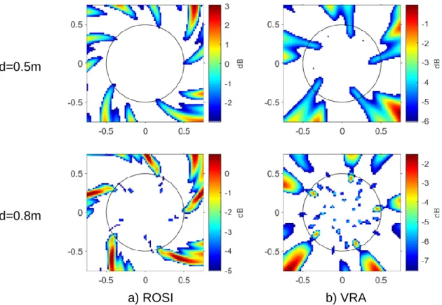
The smallest investigated distance between the source and the array plane has been selected as 𝑧 = 0.25 𝑚. As discussed earlier, this is already in the far-field of the individual sources. At this measurement distance, using a 48-microphone circular array, spatial aliasing can theoretically be avoided if the array diameter is smaller than 0.98 𝑚. Therefore, diameters of 0.5 𝑚 and 0.8 𝑚 are presented from the set of arrays used in the investigation. The results can be seen in Fig. 3. In the image, the left and the right columns (indicated by a) and b)) correspond to the two applied algorithms, with the ROSI results appearing on the left and the VRA results appearing on the right. Each row corresponds to a different array diameter, with the values marked to the left of the row. A black circle indicates the path of the sources. The 5 sources are placed equidistantly along the circle, having one at 0.5, 0 , i.e. in case of
9
successful beamforming, there are 5 noise sources localized equidistantly around the black circle, having one at 0.5, 0 .
All the beamforming maps have been normed with the source amplitude. In this synthetic environment, the sources can be guaranteed to be point sources, their strength and the radiation characteristics are controlled, and the investigated gridpoints can be chosen according to the source positions. For this reason, it can be said that the source amplitudes are reconstructed accurately if the sources have values of 0 𝑑𝐵. The color-scaled dynamic range is indicated on every map.
Using the 0.5 𝑚 diameter array, neither algorithm has been able to accurately identify the sources (first row), showing 5 large lobes which pass through the true positions, but do not peak there. Using an array having a diameter of 0.8 𝑚, the results have not improved drastically. Both algorithms have identified five stronger lobes, but these peak at positions other than the actual source positions, although in the case of the VRA, there are local maxima at the true positions. Though not presented here, the arrays of smaller and larger diameters behaved similarly, and thus, at 𝑧 = 0.25 𝑚 neither algorithm proved to be suitable for localizing the sound sources.
d=0.5m
d=0.8m
a) ROSI b) VRA
Fig. 3. The beamforming maps investigated from 𝑧 = 0.25 𝑚. The numbers on the left indicate the diameters of the arrays in the corresponding rows. Column a) shows the results obtained with the ROSI algorithm, and b) results obtained with the VRA algorithm.
10
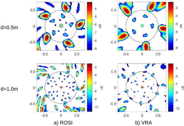
Moving further away with the array, at a distance of 𝑧 = 0.5 𝑚, spatial aliasing can theoretically be avoided below an array diameter of 1.23 𝑚. The presented array diameters are 0.5 𝑚 and 1 𝑚, as shown in the top and bottom rows of Fig. 4, respectively. In the 0.5 𝑚 diameter case, both algorithms have been able to identify five source areas, which correspond to the actual number of sources, and their positions are in the proximity of the actual positions. However, strong sidelobes can be noticed next to the source areas for both algorithms. These sidelobes are repeated every 72°, due to the symmetry of both the sources and the array. Moreover, higher beamforming values appear on the rotational axis. The results suggest that this is not a resolution issue, as the calculated spatial resolution is more than 5 times better than the distance between two sources.
In the 1 𝑚 diameter case (Fig. 4, bottom row), the false source area localized to the axis appears once again, and is even stronger, dominating the top end of the dynamic range. Other than the noise source localized to the axis, other source areas are also identified on the beamforming maps. However, many strong sidelobes appear in both cases, with the sources nearest to the true noise sources being slightly off the true positions. Thus, at 𝑧 = 0.5 𝑚 both algorithms have done a better job than at 𝑧 = 0.25 𝑚, but the obtained results still cannot truly indicate the actual source positions.
d=0.5m
d=1.0m
a) ROSI b) VRA
Fig. 4. Beamforming maps investigated from 𝑧 = 0.5 𝑚. The diameters of the arrays in the corresponding rows can be seen on the left hand side. Column a) results obtained with the ROSI algorithm, b) results obtained with the VRA algorithm.
11
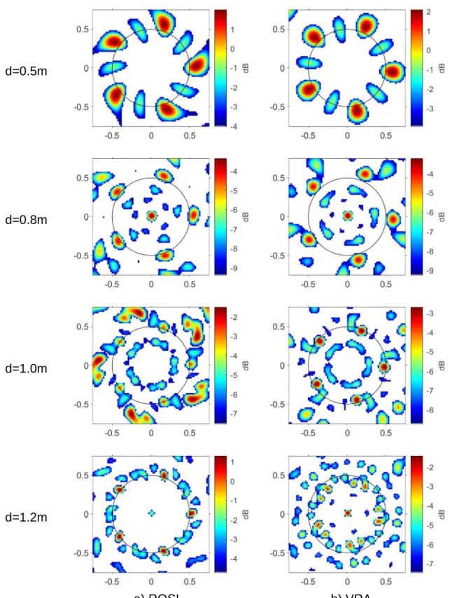
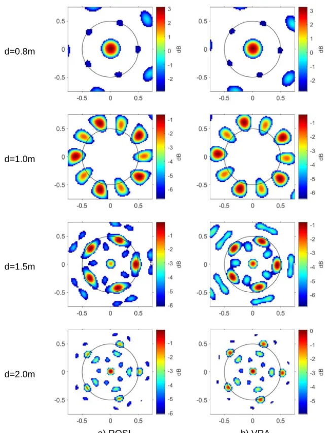
When the array is placed at 𝑧 = 1 𝑚 from the source plane, the theoretical critical array diameter is 1.95 𝑚. The noise sources are presented for four different diameter arrays: 0.5 𝑚, 0.8 𝑚, 1 𝑚, and 1.2 𝑚 (see Fig. 5). Using the 0.5 𝑚 diameter array (first row of Fig. 5), both algorithms have been able to identify five source areas in the proximity of the true positions of the sources. The sidelobes have a maximum level of approximately 3 𝑑𝐵 down from the main lobes, and they appear halfway between each neighboring pair of sources on the beamforming maps. The results of the two algorithms are quite similar to each other, although the difference between the two methods appears in the shape of the source areas.
Using the 0.8 𝑚 diameter array (second row of Fig. 5), source areas have once again been identified at the correct locations, although they are a bit off the true positions. However, a strong false source has once again appeared on the axis using both algorithms. Moreover, sidelobes have appeared on smaller as well as larger radii than the true positions. The two obtained maps are quite similar to each other in their main characteristics.
Using the 1 𝑚 diameter array (third row of Fig. 5), the ROSI algorithm has reconstructed sidelobes that exceed the true sources in strength. At the same time, the VRA algorithm has been able to identify the true positions as the strongest. Strong sidelobes appear at a smaller radial position on both maps. Both algorithms have reconstructed the same source strength at the true position, which is underestimated as compared to the true value.
Using the 1.2 𝑚 diameter array (fourth row of Fig. 5), the ROSI algorithm has been able to identify the true source positions, with the maximum sidelobe level being approximately 3 𝑑𝐵 lower. Many sidelobes are located at the same radius as the true positions, but with different circumferential positions, and there is a false source area on the axis. The source strength of the true noise source positions is overestimated. In this case, the VRA method has failed to identify the true positions. Only false source areas have been localized in an interesting pattern in the vicinity of the circumference of the true radial position. Also, there is a strong false source area on the axis. It can be stated that using the 1.2 𝑚 diameter array, the performance of the two algorithms has been significantly different.
One can note a decrease in source area with the increase of the array diameter. This is due to the resolution improvement, which is dependent of the characteristic size of the array.
Consequently, the main beamwidth decreases. This decrease in size can go down to a few grid points. This does not cause a deviation from the physical correctness in these simulation test cases, as the sources are modelled as point sources.
12 d=0.5m
d=0.8m
d=1.0m
d=1.2m
a) ROSI b) VRA
Fig. 5. Beamforming maps investigated from 𝑧 = 1 𝑚. The diameters of the arrays in the corresponding rows can be seen on the left. Column a) results of the ROSI algorithm, b) results of the VRA algorithm.
13
d=0.5m
d=1.2m
a) circular b) logarithmic spiral
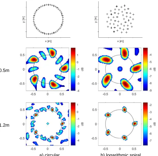
As mentioned earlier, many beamforming algorithms, including the ROSI algorithm, are better suited to a dataset recorded with a non-equidistantly spaced microphone array.
Therefore, before moving on to the next 𝑧 values, a comparison is shown between the obtained results of a ROSI simulation using a circular and a logarithmic spiral array (see Fig.
6), in order to look at the differences between them. The geometry of the spiral array has been taken from the OptiNav Array 48 system. The actual source positions have been identified using both the circular (left column) and the logarithmic spiral (right column) arrays for both presented diameters. However, the two arrays have different sidelobe characteristics. In the 0.5 𝑚 diameter case, the sidelobes appear between the actual neighboring noise source positions when the circular array is used, and one on the axis when the logarithmic spiral is used. In the 1.2 𝑚 diameter case, using the circular array results in a false source along the axis, and many sidelobes along the circumference of the true noise source positions. At the
Fig. 6. Comparison of the results of the ROSI algorithm obtained by using two different arrays. The microphone arrangements of the arrays can be seen in the top row. Column a) circular array using 48 equidistantly spaced microphones (identical with what is used throughout this article) b) logarithmic spiral array (OptiNav Array 48).
14
same time, the logarithmic spiral identified the true source positions rather well. It can be concluded that using the circular array results in more sidelobes. On the other hand, the circular array does a better job of restricting the source areas to a smaller area. Also, slight differences can be noticed in the shapes of the detected noise sources, as the sources are somewhat more stretched in the longitudinal direction in case of the logarithmic spiral array.
However, with these differences noted, conclusions may be drawn using both the circular- shaped as well as spiral-shaped arrays, as no major discrepancy can be noticed.
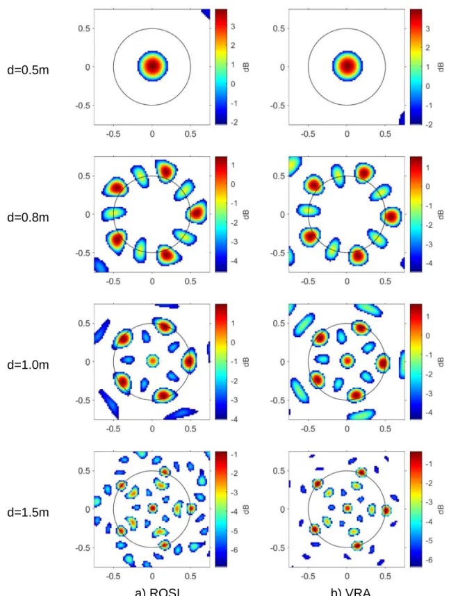
At 𝑧 = 1.75 𝑚 the critical array diameter for spatial aliasing is 3.18 𝑚, and the presented array diameters are 0.5 𝑚, 0.8 𝑚, 1 𝑚, and 1.5 𝑚 (see Fig. 7). Using the 0.5 𝑚 diameter array for data acquisition, there is only one circular noise source localized to the axis with a large beamforming value (first row of Fig. 7). If the dynamic range would be increased, the proximity of the true sources would also show local maximum values, but the obtained map is dominated by the source on the axis. This is a result of insufficient spatial resolution. As discussed in Section 4.3, spatial resolution can be determined with the help of Eq. (12), and be compared to the distance between two neighboring sources, which is 0.58 𝑚. In this case, the theoretically calculated resolution is better than this distance, being 0.49 𝑚, however, neither of the algorithms are able to distinguish between the individual sources already at this value.
Nevertheless, it is important to once again emphasize the subjectivity of the applied formula.
Using the 0.8 𝑚 diameter array, both algorithms have performed well, and their results are quite similar (second row of Fig. 7). Both have identified the source areas in the vicinities of the true positions, and they have reconstructed sources with the same beamforming levels, although somewhat overestimating the strength. Both have significant sidelobes between neighboring true source positions.
Using the 1 𝑚 diameter array (third row of Fig. 7), the performance of the two algorithms is quite similar to the previous case. Both algorithms have identified the strongest (slightly overestimated) source areas to the true positions, with the sidelobes at larger diameters being slightly stronger in case of the VRA algorithm. However, there are no strong sidelobe along the circumference of the true noise sources, but one does appear on the axis. A small difference can be noted as compared to the previous cases with regard to the peaks of the true source areas, which are located at slightly smaller radial positions than the true noise sources, instead of slightly larger radial positions. This is true for both algorithms.
Using the 1.5 𝑚 diameter array (fourth row of Fig. 7), the true sources are once again reconstructed rather well, with a less than 1 𝑑𝐵 underestimation. Sidelobes appear at both smaller as well as larger radial positions, the strongest sidelobe peaks appearing at less than 2 𝑑𝐵 below the identified source strength. Both algorithms have identified a false source on the axis. The two algorithms have performed quite similarly.
15 d=0.5m
d=0.8m
d=1.0m
d=1.5m
a) ROSI b) VRA
Fig. 7. Beamforming maps investigated from 𝑧 = 1.75 𝑚. The diameter of the arrays in the
corresponding rows can be seen on the left. Column a) results of the ROSI algorithm, b) results of the VRA algorithm.
16
At 𝑧 = 2.5 𝑚 the critical array diameter for spatial aliasing is 4.46 𝑚, and the presented array diameters are 0.8 𝑚, 1 𝑚, 1.5 𝑚, and 2 𝑚 (see Fig. 8). Using the 0.8 𝑚 diameter (first row of Fig. 8), the algorithms have been unable to identify the true source positions due to the spatial resolution constraint.
Using the 1 𝑚 diameter array (second row of Fig. 8), the actual sources have been identified, but areas which are in reality sidelobes have resulted in higher beamforming levels.
This is the situation in case of both of the algorithms. The source levels have been slightly underestimated.
Using the 1.5 𝑚 diameter array (third row of Fig. 8), both algorithms have identified the strongest source areas in the proximity of the true positions. Once again, the peaks are at a slightly smaller radius than the true noise source positions. The levels are reconstructed reasonably accurately. However, there is a false source identified on the axis. The maps of the two algorithms are quite similar.
Using the 2 𝑚 diameter array (fourth row of Fig. 8), both algorithms have identified the strongest noise sources to the axis, but have also found the true positions. The levels are 1 and 2 𝑑𝐵 off the true value for the ROSI and the VRA methods, respectively. Strong sidelobes appear at smaller radial positions, as compared to the true noise sources. The performance of the two algorithms is quite similar.
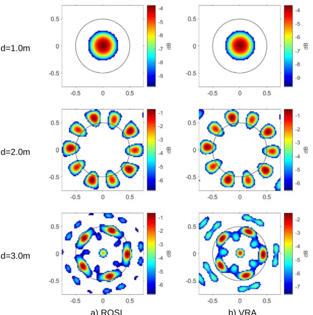
At 𝑧 = 5 𝑚 the critical array diameter for spatial aliasing is 8.79 𝑚, the investigated array diameters are 1 𝑚, 2 𝑚, and 3 𝑚 (see Fig. 9). Using the 1 𝑚 diameter array (first rows of Fig.
9), an insufficient spatial resolution results in the algorithms being unable to distinguish between the sources. Using the 2 𝑚 diameter array (second row of Fig. 9), the true sources are identified as being weaker than their sidelobes, slightly underestimating the true levels. The two algorithms have performed quite similarly in this case.
Using the 3 𝑚 diameter array (third row of Fig. 9), both algorithms have identified the true sources, slightly underestimating their strength. Both algorithms have identified a strong false source on the axis, and there are somewhat weaker sidelobes localized to smaller as well as larger radial positions. The performance of the two algorithms is similar.
17 d=0.8m
d=1.0m
d=1.5m
d=2.0m
a) ROSI b) VRA
Fig. 8. Beamforming maps investigated from 𝑧 = 2.5 𝑚. The diameters of the array in the
corresponding rows can be seen on the left. Column a) results of the ROSI algorithm, b) results of the VRA algorithm.
18 d=1.0m
d=2.0m
d=3.0m
a) ROSI b) VRA
At 𝑧 = 10 𝑚 the critical array diameter for spatial aliasing is 17.51 𝑚. This is well beyond the used array diameter set, therefore spatial aliasing is not a concern in this case. The investigated array diameters are 3 𝑚 and 5 𝑚 (see Fig. 10). Using the 3 𝑚 diameter array (first row of Fig. 10), the spatial resolution constraint proved to be a restricting factor for both algorithms, as both algorithms localized the noise sources to the axis. Using the 5 𝑚 diameter array (second row of Fig. 10), both algorithms have identified the strongest source areas to the true positions, overestimating their strengths. A false source area is identified on the axis, and other sidelobes appear at smaller and larger radial positions, as compared to the true noise source positions. The performance of the two algorithms is quite similar.
Fig. 9. Beamforming maps investigated from 𝑧 = 5 𝑚. The diameters of the array in the corresponding rows can be seen on the left. Column a) results of the ROSI algorithm, b) results of the VRA algorithm.
19 d=3.0m
d=5.0m
a) ROSI b) VRA
5 CONCLUSIONS
In this article, two algorithms have been investigated, which have different approaches in their motion compensation. One redefines the source distance at every time instant, while the other interpolates between the microphones to generate a virtually stationary measurement. A simulation test case has been defined, and the two algorithms have been tested specifically for coherent tonal noise sources. The same sources in the same arrangement have been investigated from the near vicinity of the sources to a reasonably large distance, using the same array geometry but different array diameters. The array geometry is an evenly spaced circular array, which is needed in applying the VRA algorithm. This geometry is less favorable for the ROSI algorithm, however, the results have been checked with a more suitable geometric arrangement. The behavior of the two algorithms is quite similar in many instances, with 3 or 4 exceptions out of the 21 presented cases, the results show good agreement, with regard to noise source localization as well as strength. This is undeniably good news in terms of the overall confidence in the results obtained with either algorithm.
However, this makes the VRA algorithm the more favorable choice, as working in the frequency domain, this algorithm requires a fraction of the computational effort as compared to the ROSI algorithm.
Evaluating the obtained results, it can be concluded that the sources are hardly identifiable when the array has been placed in the near vicinity of the sources. On the other end, the spatial resolution becomes an issue as one approaches the Rayleigh criterion (Eq. 12). In
Fig. 10. Beamforming maps investigated from 𝑧 = 10 𝑚. The diameters of the arrays in the
corresponding rows can be seen on the left side. Column a) results obtained with the ROSI algorithm, b) results obtained with the VRA algorithm.
20
between the two, the true sources can be more or less identified. The results could be improved by using a more advanced beamforming method on the compensated microphone data, applying deconvolution. It is expected that it would decrease the sidelobe level.
However, in many cases, when the true noise sources could be identified, a false noise source has also been identified on the rotational axis.
6 ACKNOWLEDGEMENTS
This investigation has been supported by the Hungarian National Research, Development and Innovation Centre under contract No. K 119943, and the János Bolyai Research Scholarship of the Hungarian Academy of Sciences, by the ÚNKP-19-4 New National Excellence Program of the Ministry for Innovation and Technology, by the Higher Education Excellence Program of the Ministry of Human Capacities in the frame of Water science &
Disaster Prevention research area of Budapest University of Technology and Economics (BME FIKP-VÍZ), and by the National Research, Development and Innovation Fund (TUDFO/51757/2019-ITM, Thematic Excellence Program). The publication of the results has been supported by the Hungarian National Research, Development and Innovation Centre under contract No. K 129023.
REFERENCES
[1] R.P. Dougherty. “Beamforming in acoustic testing.” in Aeroacoustic Measurements, edited by T. J. Mueller, pp. 62–97, Springer, Berlin, 2002.
[2] P. Sijtsma, S. Oerlemans and H. Holthusen. “Location of rotating sources by phased array measurements.”, AIAA 2001-2167, 2001. 7th AIAA/CEAS Aeroacoustics Conference and Exhibit, Maastricht, Netherlands, 28-30 May 2001.
doi:10.2514/6.2001-2167.
[3] O. Minck, N. Binder, O. Cherrier, L. Lamotte and V. Budinger. “Fan noise analysis using a microphone array.”, Fan 2012 - International Conference on Fan Noise, Technology, and Numerical Methods, Senlis, France, 18-20 April 2012.
[4] G. Herold and E. Sarradj. “Microphone array method for the characterization of rotating sound sources in axial fans.”, Noise Control Engineering Journal, 63, 6, 546-551, 2015.
doi:10.3397/1/376348.
[5] W. Pannert and C. Maier, “Rotating beamforming – motion-compensation in the frequency domain and application of high-resolution beamforming algorithms.”, Journal of Sound and Vibration, 333, 7, 1899-1912, 2014. doi:10.1016/j.jsv.2013.11.031.
[6] P. Sijtsma. “Using phased array beamforming to locate broadband noise sources inside a turbofan engine.”, NLR-TP-2006-320, National Aerospace Laboratory Executive summary, 2006.
[7] A.P. Dowling and J.E. Ffowcs Williams. “Sound and Sources of Sound.”, John Wiley &
Sons, New York, 1983.
[8] G. Herold, C. Ocker, E. Sarradj and W. Pannert. “A Comparison of Microphone Array Methods for the Characterization of Rotating Sound Sources.”, BeBeC-2018-D22, 2018. URL http://www.bebec.eu/Downloads/BeBeC2018/Papers/BeBeC-2018-D22.pdf, Proceedings on CD of the 7th Berlin Beamforming Conference, 5-6 March 2018.
21
[9] J.J. Christensen and J. Hald. “Beamforming.”, BV0056, Technical Review No. 1, Brüel
& Kjær, 2004.
[10] B. Tóth and J. Vad. “Algorithmic localization of noise sources in the tip region of a low-speed axial flow fan.”, Journal of Sound and Vibration, 393, 425-441, 2017.
doi:10.1016/j.jsv.2017.01.011.
[11] T. Benedek and J. Vad. “Study on the effect of inlet geometry on the noise of an axial fan, with involvement of the phased array microphone technique.”, GT2016-57772, 2016. ASME Turbo Expo 2016: Turbomachinery Technical Conference and Exposition, Seoul, South Korea, 13–17 June 2016. doi:10.1115/GT2016-57772.
[12] R.P. Dougherty, R.C. Ramachandran and G. Raman. “Deconvolution of sources in aeroacoustic images from phased microphone arrays using linear programming.”, Int. J.
Aeroacoustics, 12, 7-8, 699–718, 2013. doi:10.1260/1475-472X.12.7-8.699.
[13] S. Glegg and W. Devenport. “Aeroacoustics of Low Mach Number Flows.”, Academic Press, 2017, pp. 299-302 and 315.
[14] L.E. Kinsler, A.R. Frey, A.B. Coppens and J.V. Sanders. “Fundamentals of Acoustics.”, Wiley, New York, 1982, pp. 157-159.