Annex 2. Datasets and database - Analysis of inner peripherality in Europe. PROFECY - Inner peripheries: national territories facing challenges of access to basic services of general interest - 2017

(1)

PROFECY – Processes, Features and Cycles of Inner

Peripheries in Europe

(Inner Peripheries: National territories facing challenges of access to basic services of general

interest)

Applied Research

Final Report

Annex 2. Datasets and

(2)

This applied research activity is conducted within the framework of the ESPON 2020 Cooperation Programme, partly financed by the European Regional Development Fund.

The ESPON EGTC is the Single Beneficiary of the ESPON 2020 Cooperation Programme. The Single Operation within the programme is implemented by the ESPON EGTC and co-financed by the European Regional Development Fund, the EU Member States and the Partner States, Iceland, Liechtenstein, Norway and Switzerland.

This delivery does not necessarily reflect the opinion of the members of the ESPON 2020 Monitoring Committee.

Authors

Carsten Schürmann, TCP International (Germany)

Mar Ortega-Reig, Hèctor del Alcàzar Indarte, Institute of Local Development, University of Valencia (Spain)

Gergely Tagai, Centre for Economic and Regional Studies, Hungarian Academy of Sciences (Hungary)

Advisory Group

Project Support Team: Barbara Acreman and Zaira Piazza (Italy), Eedi Sepp (Estonia), Zsolt Szokolai, European Commission.

ESPON EGTC: Marjan van Herwijnen (Project Expert), Laurent Frideres (HoU E&O), Ilona Raugze (Director), Piera Petruzzi (Outreach), Johannes Kiersch (Financial Expert).

Information on ESPON and its projects can be found on www.espon.eu.

The web site provides the possibility to download and examine the most recent documents produced by finalised and ongoing ESPON projects.

This delivery exists only in an electronic version.

Printing, reproduction or quotation is authorised provided the source is acknowledged and a copy is forwarded to the ESPON EGTC in Luxembourg.

Contact: info@espon.eu

(3)

PROFECY – Processes, Features and Cycles of Inner Peripheries in

Europe

(4)

List of Figures

Figure 2.1. Possible representation of a school in OSM. ... 4

Figure 3.1. Data types and data usage. ... 8

Figure 4.1. Overlay of Voronoi polygons (red straight lines) with true LAU-2 boundaries (green lines) (Northwest Spain). ... 20

Figure 5.1. Structure of the PROFECY geodatabase. ... 22

List of Tables

Table 2.1: Codes used to identify relevant SGIs in OSM database. ... 6

Table 3.1. GIS datasets: Overview of data collection. ... 9

Table 3.2. Statistical datasets: Overivew of data collection. ... 15

Table 3.3. Regional typologies: Overview of data collection. ... 18

Table 4.1. LAU-2 layers: Potentials and drawbacks. ... 19

Table 5.1. Contents of the tabular datasets. ... 23

(6)

Abbreviations

AD Andorra

AL Albania

BG Bulgaria

DE Deutschland (Germany)

DG Directorate General

EBM Euroboundarymap

EL Ellada (Greece)

EU European Union

FI Finland

GADM Global administrative areas GDP Gross domestic product GIS Geoinformation system(s) GP General practitioner(s) Inhab. inhabitants

IP Inner periphery, inner peripheries

KS Kosovo

LAU Local administrative units

LT Lithuania

LV Latvia

ME Montenegro

MK Macedonia

NACE Nomenclature statistique des activités économiques dans la Communauté européenne

NO Norway

NUTS Nomenclature des unités territoriales statistiques

OSM OpenStreetMap

POI Point(s)-of-interest

PPS Purchasing power standards

PT Portugal

RO Romania

RS Republic of Serbia

SGI Services-of-general-interest

SI Slovenia

TR Turkey

UK United Kingdom

UMZ Urban morphological zone(s)

WFS Web feature service

WMS Web map service

(7)

1 Introduction

This Annex provides an overview about the data gathered, the data sources used, the data formats and contents as well as the database structure which was develop as a basis for all quantitative GIS analyses.

Basically, the delineation and characterization of Inner Peripheries in Europe require different GIS datasets as well as statistical data. For both types of data, and for those datasets required for the delineation of IPs in Europe, the project team strived to compile a complete geographical coverage for the ESPON space, at the smallest spatial level possible.

Additional datasets, mostly statistical ones, that will only be used for the characterization and analysis of IPs, do not necessarily be collected for the entire ESPON space, but for the territories of the selected case studies. In order to allow for a small-scale analysis of these case study areas, these additional datasets need to be collected at very local level (preferable LAU-2) from national data sources.

The data have been gathered from various data sources, as described later in this Annex; as regards the locations of services-of-general-interest, OpenStreetMap (OSM) has been identified as the main data provider. Despite all indisputable advantages, OSM also has some drawbacks, which were taken into consideration. In this respect, PROFECY can also be seen as an explorative study of the extent to which OSM data can be used for such purposes.

Apart from OSM, many additional data sources have been utilized (see overview tables).

A special case is the compilation of a seamless LAU-2 layer. During the delineation of inner peripheries, the project team found that overlaying the grid level results with NUTS-3 regions does not reveal convincing results due to the size of the NUTS-3 regions. Therefore, overlay with LAU-2 units appeared to be the better option. ESPON provided the project team with three different LAU-2 layers, all of which including certain potentials and drawbacks.

Eventually, the project team had to compile a new seamless and comprehensive LAU-2 layer.

All collected GIS and statistical datasets have been imported into an overall GIS database in ArcGIS File Geodatabase Format. This database format allows storing multiple data formats such as point, line, and polygon GIS features, raster datasets, network datasets, matrices, and tabular data. This geodatabase is the basis for the delineation exercises, as well as the indicator production and indicator mapping, and mapping of the delineation results.

(8)

2 Utilizing the OpenStreetMap database

OpenStreetMap^a (OSM) has been identified as the major data source for locations of SGIs.

To date, it only has been rarely utilized for analytical purposes, in contrast to mapping purposes. Before enabling people to use OSM data for analyses, it is worth to describe some technical parameters of OSM.

Essentially, OSM is a collaborative project to create a free editable map of the world, aiming at establishing a geodatabase of all geographical objects. For this purposes, OSM developed a simple data structure consisting of point features and ways (i.e. lines and polygons). All real-world geographical objects will either be stored as points, or as ways in its database. In order to differentiate types of points and ways, a TYPE field is associated with the features, where each feature type is assigned a unique code.

Being a collaborative platform, the OSM database is built up and maintained by the engagement of thousands of contributors world-wide.

The main advantages of OSM are as follows:

(i) Spatial coverage: Basically, OSM covers the entire world. So, datasets for all European countries should be available from OSM.

(ii) Types of features: OSM gathers information on all real-world geographical phenomena and geographical objects, whether natural or man-made. Basically, all different types of services-of-general-interest are covered.

(iii) High spatial resolution: All geographical objects are represented with high precision with their real-world coordinates.

(iv) Actuality: Assuming that local contributors know best when changes to geographical objects occur (for instance, a new road is opened to traffic, agricultural areas converted to urban settlements, a shop is opened or closed), new real-world developments will be implemented into OSM very soon, ensuring actuality of the OSM database.

(v) Free usage: Anybody has free access to, and can use OSM data freely for non- commercial use as long as the results of his activities are also freely shared to the public.

(vi) Easy access: The OSM database can be easily accessed either by directly visiting the OSM website, or by using specific interfaces built-in into GIS software products (like WMS or WFS services based upon OSM data).

a www.openstreetmap.org

(9)

At the same time, OSM also shows some important drawbacks for using this database in PROFECY:

(i) Quality assurance: As there is no centralized quality assurance mechanism implemented in the OpenStreetMap initiative, the OSM database has problems with quality assurance with regard to the completeness and actuality of the information.

The general idea being that the local contributors at the same time ensure completeness and actuality; however, as the number of contributors in cities and regions, and their levels of engagement, vary substantially, the completeness and actuality of the information cannot be guaranteed. Experiences show that the coverage (completeness) of real-world objects in agglomerations is quite high, while in rural areas problems exist with the level of completeness. The level of activities of the OSM community also differs between countries, with some countries being highly active while in others countries only few activities exist. By way of consequence, one needs to expect differences in completeness and actuality of OSM data between regions and countries.

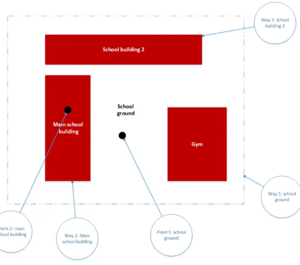
(ii) Object types: As regards SGIs, sometimes OSM has multiple entries for one facility in its database; for example, a school might be represented by one or more points and by different ways: one way for its building, another way for a side-building, and a third way representing the entire school plot. The first point may represent the school ground, and a second and third point may represent the main and the side buildings (Figure 2.1).

(10)

Figure 2.1. Possible representation of a school in OSM.

The school name may also be assigned to each way and point, but this is not guaranteed.

To make the situation even more complex, sometimes only the point(s) or only the way(s) are available in OSM, or both points and ways. Similarly, sometimes the school name is assigned properly, sometime it is missing. Thus, when downloading data from the OSM database it is not sufficient to look at point features alone, but also ways must be evaluated. In reality, sometimes there are two different schools such as a primary school and a secondary school reside on the same school ground; if the schools names are not properly assigned, it is difficult to judge whether the school objects represent one or two different schools. In addition to the geometries, therefore one has also to evaluate the names assigned to the geographical objects in OSM.

(iii) Missing detailed information: Although OSM differentiates the basic types of SGIs (i.e. schools from kindergardens, doctors from banks, shops from restaurants etc.), a further differentiation of schools into primary or secondary schools, or of doctors or hospitals into general doctors/general hospitals and specialized doctors/hospitals is quite difficult, sometimes impossible. The TYPE field does not allow for such further

(11)

differentiations; only the facility name sometimes provides such additional information (for instance, if the name of a surgery is like “Dr. Smith Dental Centre”); unfortunately, often the facility name is too general to obtain such details (“Dr. Smith”), and in many cases the facility name is not given at all or is too general (“School”). The project team thus also evaluated the NAME field to obtain additional information for a further sub-differentiation of facilities, and also looked into additioanl data sources to verify / enrich OSM information.

(iv) Multiple database entries: For larger facilities like hospitals or schools, which in real- world often have several buildings within one ground or even several locations within a city, OSM usually includes multiple entries in its database (see Figure 2.1). For instance, in case of hospitals, each hospital building may be stored in the database as separate feature. For the purpose of calculated access times to the closest facility, the multiple entries allow to model accessibility very precisely^b. By way of consequence, the number of facilities such as hospitals or schools in the OSM database may be higher compared to official statistics, which only count the administrative view.

(v) Miscodings / errors: Like in all databases, sometimes facilities are wrongly coded in the OSM database. For instance, a kindergarden or university may be coded as a school, or a bank as a shop. Options to identify such errors automatically are very limited. By comparing the facility name with the type of facility sometimes identifies such errors, but often one can only identify such errors by comparing OSM with other data sources, which is quite complex and a lenghty task given the high amount of SGI facilities.

(vi) Non-standardized names: OSM includes a NAME field to label geographical objects.

Names and labels of facilities are, however, not standardized in OSM. Sometimes facility names are abbreviated, sometimes not. Also the sequence of name parts is not standardized (i.e. Lübeck post office vs. Postamt Lübeck). Moreover, usually names are given in the national language using the national typefaces. This may sometimes, for instance in case of Cyrillic letters, lead to problems when exporting data from OSM to other databank systems when the Cyrillic letters are on-the-fly

“transformed” into something unreadable (becase the different software systems

(12)

There are no clear standards set in OSM to which facility type such cases are attributed. In the said example, preschooles may sometimes be encides as kindergarten, and another time as elementary school. This may vary from country to country, but sometimes even within countries.

Eventually, these characteristics of the OSM database lead to quite diverse situations as regards the completeness, accuracy, actuality and correctness of SGI facilities in European countries, and also with regard to the necessary steps for quality control. Details on the evaluation results are provided in the following chapter.

Due to the large amount of data to be downloaded from OSM database for the entire ESPON space, for technical reasons OSM data were not downloaded from the OSM database directly, but from the GeoFabrik Download Section^c. GeoFabrik provides pre-processed OpenStreetMap data for free download by continent and country in different data formats (OSM PBG, OSM BZ2, ArcGIS Shapefile). Download was triggered in Shapefile format.

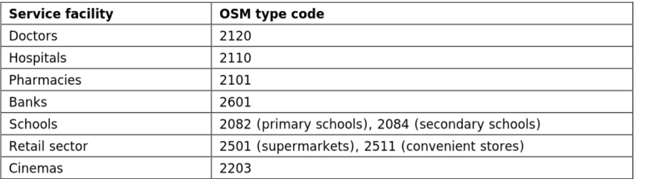
In order to identify and select the service facilities relevant for PROFECY, the following feature types were selected (Table 2.1):

Table 2.1: Codes used to identify relevant SGIs in OSM database.

Service facility OSM type code

Doctors 2120

Hospitals 2110

Pharmacies 2101

Banks 2601

Schools 2082 (primary schools), 2084 (secondary schools) Retail sector 2501 (supermarkets), 2511 (convenient stores)

Cinemas 2203

In order to set up a database on SGI facilities based upon OSM data, accounting for the curcumstances described above, the following workflow has been implemented in Python scripts on top of ArcGIS:

1. Download country packages in Shapefile format from GeoFabrik server.

2. Uncompressing data packages

3. Select all point POIs from POI point layer with the relevant code(s) (see Table 1) and store them as new layers

4. Merge the individual country-wise point layers into one overall point layer covering the entire ESPON space.

c http://download.geofabrik.de/

(13)

5. Select all polygon POIs from POI polygon layer with the relevant code(s) and store them as new layers.

6. Merge the individual country-wise polygon layers into one overall polygon layer covering the entire ESPON space.

7. Check whether the polygons are already represented as points in OSM. If yes, neglect that polygon; if not, add the polygon centroid to the point layer as additional point.

8. Select all buildings with the relevant type from the buildings polygon layer.

9. Merge the individual country-wise building layers into one overall building layer covering the entire ESPON space.

10. Check whether the buildings are already represented as points in OSM. If yes, neglect the building; if not, add the building centre to the point layer as additional point.

11. Further differentiate doctors, hospitals, schools and retail facilities by evaluating the facility names. Remove facilities that are of no relevance for PROFECY (for instance, dentists from the doctors dataset).

12. Compile additional data sources to complement or verify the OSM database.

13. Check OSM data against additional data sources, and edit OSM data as needed.

The above basic workflow was implemented for each type of SGI individually, with some slight modifications for each type. Steps 1 to 10 were completely implemented in form of automated Python scripts (by using ArcPy funtions); the remaining steps 11, 12 and 13, however, were to a large degree based upon additional manual works.

(14)

3 Data collection overview

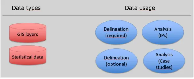
Basically, the PROFECY team compiled GIS layers and statistical data (Figure 3.1). The data were used for varios purposes, such as datasets required for delineation and optional datasets to be used in the delineation process, data used for the analyses of IP regions in Europe, so as datasets used solely in the case study analysis. Some datasets were used for different purposes, while others were used for one specific purpose only.

Figure 3.1. Data types and data usage.

The following tables provide final overviews about the collectedl data for GIS datasets (Table 3.1) and statistical datasets (Table 3.2), as well as on regional typologies (Table 3.3).

Although the project team tried to compile a complete coverage of all ESPON countries for all selected SGIs, based on OSM and additional sources, some data gaps remain for some countries. The following table will indicate these cases.

(15)

3.1 Data sources for GIS datasets

Abbreviations used in column USAGE of the following tables:

D = delineation

A = analysis of IP regions (o) = optional datasets (r) = required datasets

(cs) = optinal datasets for case studie regions

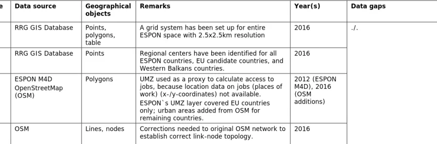
Table 3.1. GIS datasets: Overview of data collection.

Dataset Usage Data source Geographical

objects Remarks Year(s) Data gaps

Grid system D (r) RRG GIS Database Points, polygons, table

A grid system has been set up for entire

ESPON space with 2.5x2.5km resolution 2016 ./.

Regional centres D (r) RRG GIS Database Points Regional centers have been identified for all

ESPON countries, EU candidate countries, and 2016

(16)

Rail network RRG GIS Database

Corine land cover A (cs) EEA Polygons Can be used as part of the case studies to

characterize the case study areas 1990, 2000, 2006 NUTS-3 region

layer D (r) /

A (r) ESPON Database RRG GIS Database

Only tentative version was available from ESPON with certain drawbacks; therefore, a new layer was generated.

NUTS 2013 classification NUTS 2010 classification

ESPON layer covered only EU Member States with poor resolution.

LAU-2 A ESPON,

Euroboundarymap (EBM), Global Administrative Areas (GADM)

ESPON provided three different LAU-2 datasets, each with certain drawbacks and data gaps; gaps filled by combining different ESPON datasets and by using additional GADM layers

2011, 2013 (ESPON/EBM) 2016 (GADM)

For further details see Chapter 4

Highway ramps RRG GIS Database Points Will not be used for delineation purposes, but only for analyses of IP regions.

Indicator on density of highway ramps per NUTS-3 region and per inhabitant generated for analyzing IP regions.

2016 ./.

Train stations D (r) All passenger train stations used for

delineating IP areas

Indicator on density of train stations per NUTS-3 region and per inhabitant generated for analyzing IP regions.

Doctors D (r) /

A OSM, plus additional data sources for verification for Andorra, Estonia, Croatia, Denmark, Germany (partly), Hungary, Iceland, Spain and Sweden

Focus was given on general practitioners (GPs) and general surgeries; specialized doctors excluded.

Indicator on density of doctors per NUTS-3 region and per inhabitant generated for analyzing IP regions.

2016 (latest data available in OSM)

OSM database very incomplete for the following countries: AD, AL, BG, EL, FI, KS, LT, LV, ME, MK, NO, PT, RO, RS, SI, TR

(17)

Hospitals OSM, plus

additional data sources for verification for Croatia, Estonia, Finland, Germany, Hungary, Iceland, Latvia, Lithuania, Romania, Slovakia, Slovenia, Spain.

Focus was given on general hospitals;

specialized facilities such as wellness clinics, hospices, etc. were excluded.

Indicator on density of hospitals per NUTS-3 region and per inhabitant generated for analyzing IP regions.

Pharmacies OSM, plus

additional data sources for verification for Croatia, Germany, Hungary, Iceland, Romania

Indicator on density of pharmacies per NUTS-3 region and per inhabitant generated for analyzing IP regions.

Schools OSM,

OpenEducation Europe, Enic- naric.net,

EuroEducation.net (used to

differentiate

Focus given on primary and secondary schools. In fact, primary schools and secondary schools were treated as two separate SGIs.

Vocational schools and other training centers, and tertiary schools excluded.

Indicator on density of secondary and primary

(18)

Retail:

supermarkets and convenient stores

Both supermarkets and convenient stores compiled and used for delineation.

Indicator on density of supermarkets and convenient stores per NUTS-3 region and per inhabitant generated for analyzing IP regions.

Data on shopping centres and malls have not been compiled, since these facilities typically are not used for daily goods supply but for medium to long-run goods. If supermarkets or convenient stores are located inside such centres or malls, they shall be included in OSM anyway.

Banks Only bank offices considered; locations of cash

machines excluded.

Indicator on density of banks per NUTS-3 region and per inhabitant generated for analyzing IP regions.

2016 (latest data available in OSM)

(19)

Additional data sources have been searched and identified in order to complement OSM data on SGI locations. The difficulty being that these additional data sources need to provide complete address information of the facilities, which is not always the case. Sometimes, additional data sources focus on statistical measures (for instance, giving the number of primary school per region), but without indicating the location. In the light of these challenges, the following additional data sources have been used to completment the OSM data on services-of-general-interest:

Doctors:

• Hungarian Ministry of Health (2017)

• SNS – Servico Nacional de Saude (2017)

• Croatia Ministry of Health (2017)

• 1177 Vardguiden for Sweden (2017, www.1177.se)

• Sundhed DK for Denmark (2017, www.sundhed.dk)

• Eesti Haigekassa (2017, www.haigekassa.ee)

• Ministry of Welfare Iceland (2016)

• Principality of Liechtenstein (2017, https://en.welcome.li/liechtenstein-doctor-128.html) Despite these effords, after a final evaluation the project team identified a number of countries for which the doctor´s database still appears to be to poor for further analyses: Albania, Bosnia-Hercegovina, Bulgaria, Greece, Finland, Latvia, Lithuania, Macedonia, Montenegro, Malta, Norway, Romania, Republic of Serbia, and Turkey.

Hospitals:

• Catalogue of World Hospitals (2011): Ranking web of World Hospitals - Hospitals of Latvia. http://hospitals.webometrics.info/hospital_by_country.asp?country=lv

• Croatian Health Insurance Fund (2017): Croatian health care system. www.hzzo.hr

(20)

• Kurklinikverzeichnis (ed.) (2017): Kurklinik Verzeichnis, Rehakliniken, Kurkliniken und Mutter/Vater-Kind-Kuren. www.kurklinikverzeichznis,de. Baden-Baden: Jan Malek.

• Lietuvos Medicina (2012): List of Hospitals and Clinics. www.medicina.lt

• Ministerul Sănătății (2017): List of hospitals in Romania. www.data.gov.ro

• Ministry of Welfare Iceland (2016)

• Slovenian Ministry of Health (2017)

• STMAS (2009): Bayerisches Krankenhausregister und Krankenhausplan.

• Wikipedia (2012a): List of Hospitals in Estonia.

http://en.wikipedia.org/wiki/List_of_hospitals_in_Estonia

• Wikipedia (2012b): List of Hospitals in Latvia.

http://en.wikipedia.org/wiki/List_of_hospitals_in_Latvia

• Wikipedia (2012c): List of Hospitals in Lithuania.

http://en.wikipedia.org/wiki/List_of_hospitals_in_Lithuania

These sources have been used to complement OSM information, and to further attribute hospitals in order to separate general hospitals from specialized clinics.

Pharmacies:

• Croatia Health Insurance Fund, 2017

• Icelandic Medicines Agency, Lyfja.is, LMI, 2017

Primary and secondary schools:

• Bulgarian Ministry of Education and Science (2017)

• Euroguidance Österreich (2017)

• Govern d’Andorra (2017)

• Government of Macedonia (2017)

• Registro Estatal de Centros Docentes No Universitarios (Spain, 2017)

These sources have been used to complement OSM information, and to differentiate primary from secondary schools, and to exclude schools that are not relevant for PROFECY (such as vocational schools, universities of applied sciences etc.).

(21)

3.2 Data sources for statistical datasets and indicators

Statistical data will be used in PROFECY in different ways. Some of them will be used to delineate inner peripheries in Delineation 2 and Delineation 4, others will be used to analyse inner peripheries in WP 4, while some datasets will be used in detailed analyses in the case study areas.

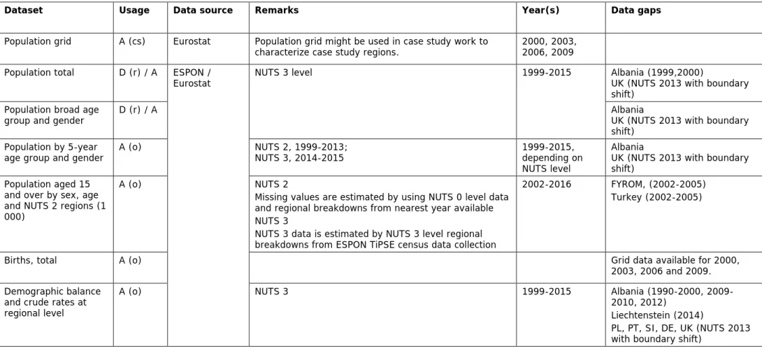
Table 3.2. Statistical datasets: Overivew of data collection.

Dataset Usage Data source Remarks Year(s) Data gaps

Population grid A (cs) Eurostat Population grid might be used in case study work to

characterize case study regions. 2000, 2003, 2006, 2009 Population total D (r) / A ESPON /

Eurostat NUTS 3 level 1999-2015 Albania (1999,2000)

UK (NUTS 2013 with boundary shift)

Population broad age

group and gender D (r) / A Albania

Population by 5-year

age group and gender A (o) NUTS 2, 1999-2013;

NUTS 3, 2014-2015 1999-2015,

depending on NUTS level

Albania

Population aged 15 and over by sex, age and NUTS 2 regions (1 000)

A (o) NUTS 2

Missing values are estimated by using NUTS 0 level data and regional breakdowns from nearest year available NUTS 3

2002-2016 FYROM, (2002-2005) Turkey (2002-2005)

(22)

Dataset Usage Data source Remarks Year(s) Data gaps Net Migration total (+

statistical adjustment) A (o) NUTS3 1999-2015 Albania

Net Migration by 5- year age group (+

statistical adjustment)

NUTS 2, 1999-2013;

NUTS 3, 2014 1999-2014,

depending on NUTS level

Albania

PL, PT, SI, DE, UK (NUTS 2013 with boundary shift)

GDP grid A (o) ESPON

database GDP (€ and PPS), total population, births, deaths 2000, 2003, 2006, 2009 GDP at current market

prices by Million €, Million PPS; PPS /Inhab

D (r) / A

(r) ESPON /

Eurostat NUTS 3

Missing NUTS 3 values are estimated by using NUTS 0 or NUTS 2 level data and regional breakdowns from nearest year available

2000-2015 Iceland, Liechtenstein, Montenegro, Switzerland, Turkey

Gross value added at

basic prices A (o) NUTS 3

2000-2015 Iceland, Liechtenstein, Montenegro, Switzerland, Turkey

Albania (2000-2007, 2015) Belgium (2000-2002) Norway (2000-2010, 2015) Employment by sex,

broad age groups (1000 and %); by age, economic activity (NACE Rev. 2) – 1 000

A (o) NUTS 3

2000-2014 Albania, Iceland, Liechtenstein, Montenegro, Switzerland, Turkey

France (C – Manufacturing) Belgium (2000-2002) Finland (2014) Croatia (2000-2008) Hungary (2000-2007, 2014) FYROM (2000-2009, 2014) Norway (2000-2010, 2014) Portugal (NUTS 2013 with boundary shift)

(23)

Dataset Usage Data source Remarks Year(s) Data gaps Economically active

population by sex, age and NUTS 2 regions (1000)

A (o) ESPON /

Eurostat NUTS 2

NUTS 3 data is estimated by NUTS 3 level regional breakdowns from ESPON TiPSE census data collection

2002-2016 FYROM, (2002-2005) Turkey (2002-2005)

Unemployment by sex, age and NUTS 2 regions (1 000)

A (o) ESPON /

Eurostat NUTS 2

NUTS 3 data is estimated by NUTS 3 level regional breakdowns from ESPON TiPSE census data collection

2002-2016 FYROM, (2002-2005) Turkey (2002-2005)

Long-term

unemployment (12 months and more)

A (o) Eurostat NUTS 2 2002-2016 FYROM, (2002-2005)

Turkey (2002-2005) Young people neither

in employment nor in education and training by sex and NUTS 2 regions (NEET rates)

A (o) Eurostat NUTS 2 2002-2016 FYROM, (2002-2005)

Turkey (2002-2005)

Population aged 25-64

by educational A (o) Eurostat NUTS 2 2002-2016 FYROM, (2002-2005)

Turkey (2002-2005)

(24)

Dataset Usage Data source Remarks Year(s) Data gaps Jobs D (r) ./. Detailed European-wide dataset for NUTS-3 regions not

available; replaced with dataset on urban morphological zones (see above)

Accessibility potential

by road and rail ESPON

MATRICES project

Standardized index values as well as unstandardized

raw data at NUTS-3 level obtained. 2001, 2006, 2011, 2014

Further statistical data collected at lower spatial scale, such as LAU-2 and LAU-1, for case studies, which are not listed here.

3.3 Regional typologies

PROFECY will use different existing regional typologies to compare them with the results of the delineation of inner peripheries. To what extent overlap specific regions with IP areas? Where are similarities? Where are differences?

Table 3.3. Regional typologies: Overview of data collection.

Dataset Usage Data source Remarks Data gaps

Urban-rural typology A (r) DG Regio / via

ESPON Covers EU countries, Iceland, Norway, Switzerland and Turkey Non-EU Balkan countries

Metropolitan regions Non-EU countries

Mountains and islands

(25)

4 LAU-2 layer

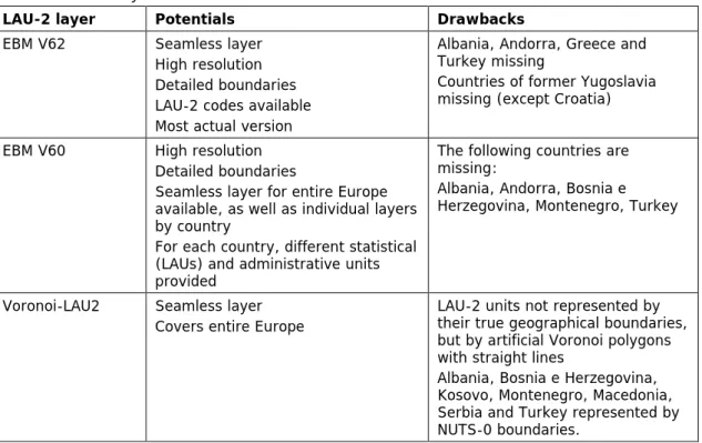
ESPON provided the projec team with three different LAU-2 layers, which were the EuroBoundaryMap V. 62 (EBM V62 for 2013), the EuroBoundarymap V. 60 for 2011 (EBM V60) and the Voronoi-LAU2 layer produced by ESPON itself. All these three layers have certain potentials and drawbacks, as summarized in Table 4.1.

Table 4.1. LAU-2 layers: Potentials and drawbacks.

LAU-2 layer Potentials Drawbacks

EBM V62 Seamless layer High resolution Detailed boundaries LAU-2 codes available Most actual version

Albania, Andorra, Greece and Turkey missing

Countries of former Yugoslavia missing (except Croatia)

EBM V60 High resolution Detailed boundaries

Seamless layer for entire Europe available, as well as individual layers by country

For each country, different statistical (LAUs) and administrative units provided

The following countries are missing:

Albania, Andorra, Bosnia e Herzegovina, Montenegro, Turkey

Voronoi-LAU2 Seamless layer Covers entire Europe

LAU-2 units not represented by their true geographical boundaries, but by artificial Voronoi polygons with straight lines

Albania, Bosnia e Herzegovina, Kosovo, Montenegro, Macedonia, Serbia and Turkey represented by NUTS-0 boundaries.

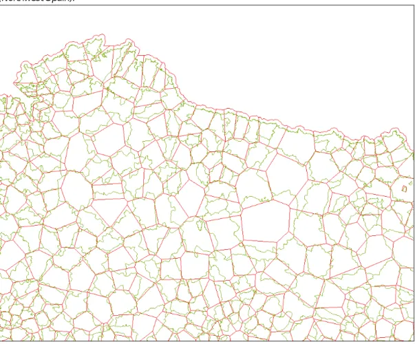
The EBM V61 layer seem basically very useful for PROFECY in terms of resolution and boundary details; the only drawback being the missing countries. The same can be said about the EBM V60 layer. The Voronoi layer is, in contrast to the previous two, not suitable for PROFECY as it does not provide the true LAU-2 boundaries but artifical Voronoi polygons. An overlay of these polygons with the true boundaries from EBM V62 layer reveals this drawback (Figure 4.1 examplifies this for Northwest Spain).

(26)

Figure 4.1. Overlay of Voronoi polygons (red straight lines) with true LAU-2 boundaries (green lines) (Northwest Spain).

In order to obtain a comprehensive coverage for all ESPON countries, the EBM V62 layer has been taken as a starting point. Additional LAU-2 boundaries for Greece, Kosovo and Macedonia have been taken from trh EBM V60 layer; for the remaining missing countries (Albania, Andorra, Bosnia e Herzegovina, Montenegro, Turkey) layers from the Global Administrative Areas Database (GADM) have been downloaded⁴ and processed.

Although the resolution of the GADM datasets is not that high as the EuroBoundaryMap, and data for Turkey are at district level only, these drawbacks were considered acceptable in order to obtain a seamless LAU-2 layer for entire ESPON space.

4 Datasets can be downloaded from GADM free for academic and other non-commercial uses. Website:

www.gadm.org. Download section by country: www.gadm.org/country

(27)

5 The PROFECY Geodatabase

As the Delineations 1 and 3 rely on grid-based approaches for the entire ESPON space, it is anticipated that a large amount of data will be generated. To efficiently compile, handle, and store these large datasets, an ArcGIS File Geodatabase has been implemented.

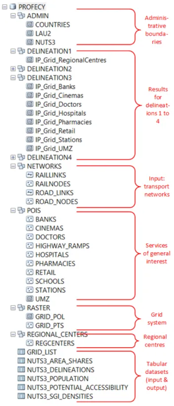
This geodatabase stores all required input data, temporal interim data sets, and all output data. The name of the database is PROFECY; it is subdivided into nine feature datasets, plus several tables (Figure 5.1. Structure of the PROFECY geodatabase.Figure 5.1).

The nine feature datasets store various feature classes on administrative boundaries (ADMIN), the results of the four delineation approaches (DELINEATION1, DELINEATION2, DELINEATION3, and DELINEATION4), the required input road and rail transport networks (line and point feature classes, NETWORKS), point and polygon feature classes for the services-of-general-interest (POIS), the grid system (RASTER), and regional centres (REGIONAL_CENTRES). In addition to these feature datasets, a number of tables are also stored in the geodatabase to provide statistical input data (NUTS3_POPULATION, NUTS3_POTENTIAL_ACCESSIBILITY) required for the delineation of inner peripheries, and to store indicators (NUTS3_SGI_DENSITIES) and delineation results at grid level (GRID_LIST) and NUTS-3 level (NUTS3_AREA_SHARES, NUTS3_DELINEATIONS).

Temporal datasets generated by scripts will also be stored within this database, but will be removed immediately after the final output has been produced, in order to keep the geodatabase as small and compact as possible.

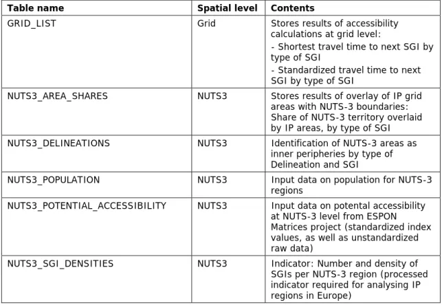
Further details on the contents of the tabular datasets are listed in Table 5.1.

The projection parameters of the PROFECY geodatabase are as follows:

Projection: Lambert Datum: (none) Units: Meter Spheroid: Clarke1866 1st standard parallel: 27 0 0.000 2nd Standard parallel: 63 0 0.000 Central meridian: 10 0 0.000 Latitude of projection’s origins: 52 0 0.000 False easting (meters): 0.000 False northing (meters): 0.000

(28)

Figure 5.1. Structure of the PROFECY geodatabase.

(29)

Table 5.1. Contents of the tabular datasets.

Table name Spatial level Contents

GRID_LIST Grid Stores results of accessibility

calculations at grid level:

- Shortest travel time to next SGI by type of SGI

- Standardized travel time to next SGI by type of SGI

NUTS3_AREA_SHARES NUTS3 Stores results of overlay of IP grid areas with NUTS-3 boundaries:

Share of NUTS-3 territory overlaid by IP areas, by type of SGI NUTS3_DELINEATIONS NUTS3 Identification of NUTS-3 areas as

inner peripheries by type of Delineation and SGI

NUTS3_POPULATION NUTS3 Input data on population for NUTS-3 regions

NUTS3_POTENTIAL_ACCESSIBILITY NUTS3 Input data on potental accessibility at NUTS-3 level from ESPON Matrices project (standardized index values, as well as unstandardized raw data)

NUTS3_SGI_DENSITIES NUTS3 Indicator: Number and density of SGIs per NUTS-3 region (processed indicator required for analysing IP regions in Europe)

(30)

ESPON 2020 – More information ESPON EGTC

4 rue Erasme, L-1468 Luxembourg - Grand Duchy of Luxembourg Phone: +352 20 600 280

Email: info@espon.eu

www.espon.eu, Twitter, LinkedIn, YouTube

The ESPON EGTC is the Single Beneficiary of the ESPON 2020 Cooperation Programme. The Single Operation within the programme is implemented by the ESPON EGTC and co-financed by the European Regional Development Fund, the EU Member States and the Partner States, Iceland, Liechtenstein, Norway and Switzerland.