Annex 8. Analysis of inner peripherality in Europe. PROFECY - Inner peripheries: national territories facing challenges of access to basic services of general interest - 2017

(1)

PROFECY – Processes, Features and Cycles of Inner

Peripheries in Europe

(Inner Peripheries: national territories facing challenges of access to basic services of general

interest)

Applied Research

Final Report

Annex 8. Analysis of inner

peripherality in Europe

(2)

This applied research activity is conducted within the framework of the ESPON 2020 Cooperation Programme, partly financed by the European Regional Development Fund.

The ESPON EGTC is the Single Beneficiary of the ESPON 2020 Cooperation Programme. The Single Operation within the programme is implemented by the ESPON EGTC and co-financed by the European Regional Development Fund, the EU Member States and the Partner States, Iceland, Liechtenstein, Norway and Switzerland.

This delivery does not necessarily reflect the opinion of the members of the ESPON 2020 Monitoring Committee.

Authors

Gergely Tagai, Annamária Uzzoli, Bálint Koós, Centre for Economic and Regional Studies, Hungarian Academy of Sciences (Hungary)

Mar Ortega-Reig, Hèctor del Alcàzar, Institute for Local Development, University of Valencia (Spain)

Advisory Group

Project Support Team: Barbara Acreman and Zaira Piazza (Italy), Eedi Sepp (Estonia), Zsolt Szokolai, European Commission.

ESPON EGTC: Marjan van Herwijnen (Project Expert), Laurent Frideres (HoU E&O), Ilona Raugze (Director), Piera Petruzzi (Outreach), Johannes Kiersch (Financial Expert).

Information on ESPON and its projects can be found on www.espon.eu.

The web site provides the possibility to download and examine the most recent documents produced by finalised and ongoing ESPON projects.

This delivery exists only in an electronic version.

Printing, reproduction or quotation is authorised provided the source is acknowledged and a copy is forwarded to the ESPON EGTC in Luxembourg.

Contact: info@espon.eu

(3)

PROFECY – Processes, Features and Cycles of Inner Peripheries in

Europe

(4)

List of Figures

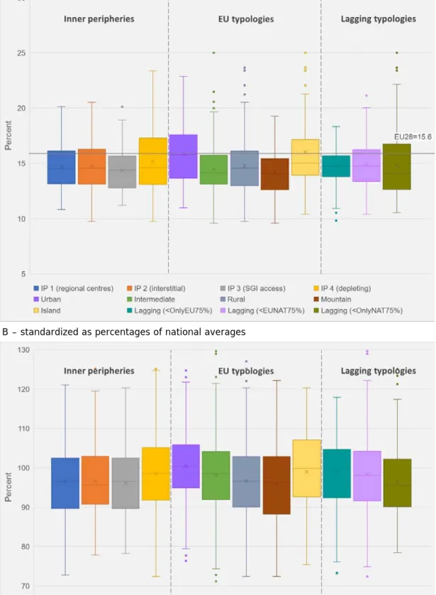
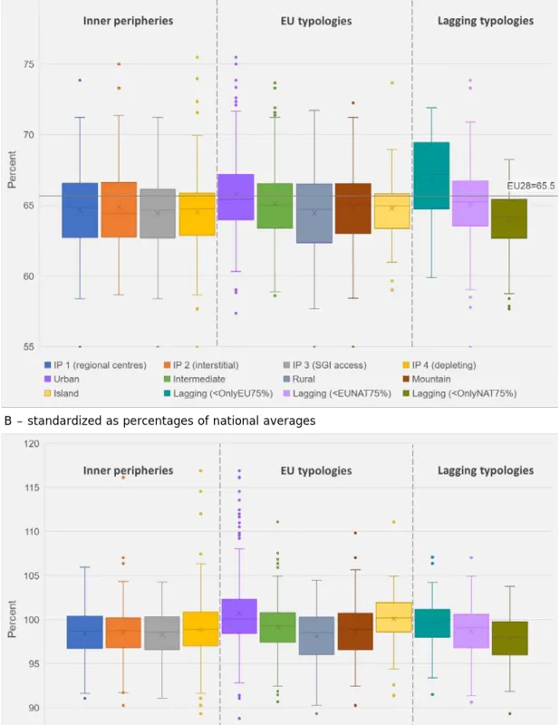
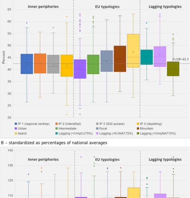
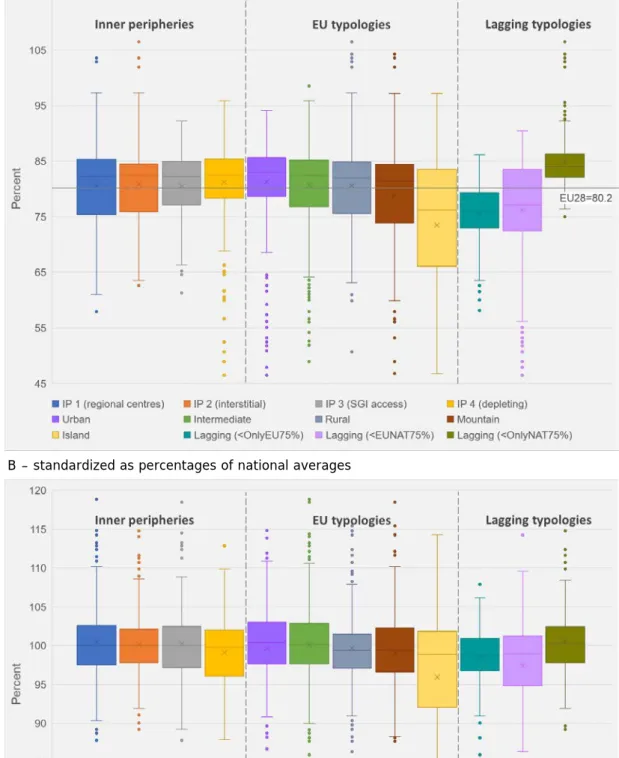
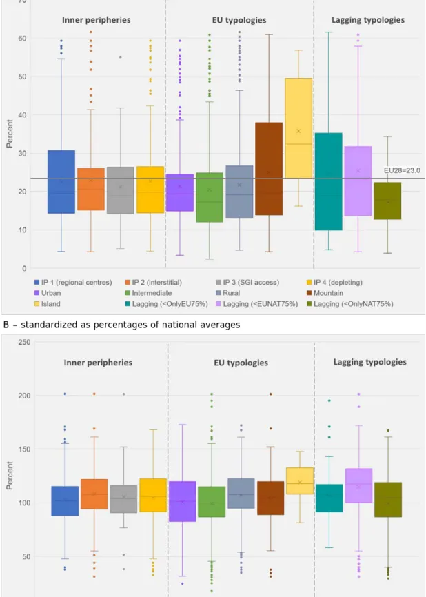
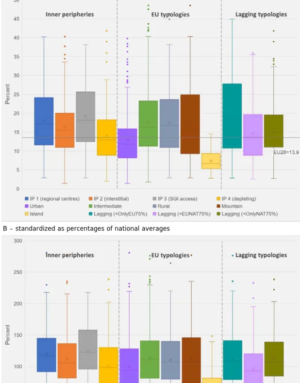
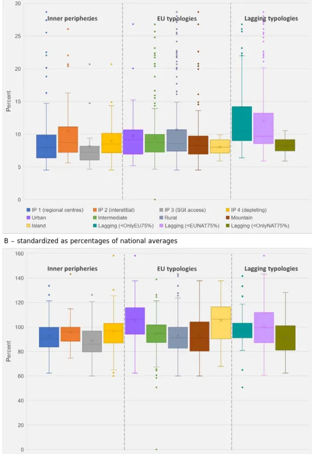
Figure 1.1: Lagging region typologies used in ESPON PROFECY project ... 5 Figure 1.2: Inner peripheries counted by different types and by the ‘union’ of different delineations ... 9 Figure 3.1: The interpretation of a box plot chart ... 43 Figure 3.2: Ratio of child age (0-14) population in Europe by IP delineations and EU regional typologies, 2015... 46 Figure 3.3: Ratio of working age (15–64) population in Europe by IP delineations and EU regional typologies, 2015 ... 50 Figure 3.4: Old age dependency rate in Europe by IP delineations and EU regional typologies, 2015 ... 54 Figure 3.5: Inactivity rate (15+) in Europe by IP delineations and EU regional typologies, 2016 ... 58 Figure 3.6: Gender gap in activity (female/male) in Europe by IP delineations and EU regional typologies, 2016... 62 Figure 3.7: Unemployment rate (15+) in Europe by IP delineations and EU regional typologies, 2016... 66 Figure 3.8: Ratio of population (25-64) with low qualification (ISCED0-2) in Europe by IP delineations and EU regional typologies, 2016 ... 70 Figure 3.9: GDP (PPS) per inhabitant in percentage of the EU average in Europe by IP delineations and EU regional typologies, 2015 ... 74 Figure 3.10: Gross value added per employed person in Europe by IP delineations and EU regional typologies, 2014 ... 78 Figure 3.11: Ratio of employed persons working in manufacturing industry (NACE Rev.2 C) in Europe by IP delineations and EU regional typologies, 2014 ... 81 Figure 3.12: Number of active enterprises per 10000 persons in Europe by IP delineations and EU regional typologies, 2013 ... 85 Figure 3.13: Birth rate of enterprises (compared to the number of active enterprises) in Europe by IP delineations and EU regional typologies, 2013 ... 88 Figure 3.14: Three year survival rate of enterprises (born in t-3) in Europe by IP delineations and EU regional typologies, 2013 ... 91 Figure 3.15: Density of retail units in Europe by IP delineations and EU regional typologies, 2016 ... 95

(7)

Figure 3.16: Density of hospitals in Europe by IP delineations and EU regional typologies, 2016 ... 98 Figure 3.17: Density of primary schools in Europe by IP delineations and EU regional typologies, 2016... 102 Figure 4.1: Basic trends in dynamics of inner peripheries regarding population change, 2000–

2015 (population in year 2000 = 100%) ... 110 Figure 4.2: Basic trends in dynamics of inner peripheries regarding change of net migration rate, 2000–2015 (migrant population in year 2000 = 100%) ... 114 Figure 4.3: Position shifts of NUTS 3 regions in Europe regarding old age dependency rate, 2000–2015 ... 116 Figure 4.4: Basic trends in dynamics of inner peripheries regarding old age dependency rate, 2000–2015 ... 117 Figure 4.5: Position shifts of NUTS 3 regions in Europe regarding inactivity rate (15+), 2002–

2016 ... 120 Figure 4.6: Basic trends in dynamics of inner peripheries regarding inactivity rate (15+), 2002–2016 ... 121 Figure 4.7: Position shifts of NUTS 3 regions in Europe regarding unemployment rate (15+), 2002–2016 ... 124 Figure 4.8: Basic trends in dynamics of inner peripheries regarding unemployment rate (15+), 2002–2016 ... 125 Figure 4.9: Position shifts of NUTS 3 regions in Europe regarding ratio of population (25–64) with low qualification (ISCED 0–2), 2002–2016 ... 128 Figure 4.10: Basic trends in dynamics of inner peripheries regarding ratio of population (25–

64) with low qualification (ISCED 0–2), 2002–2016 ... 129 Figure 4.11: Position shifts of NUTS 3 regions in Europe regarding GDP per inhabitant (PPS), 2000–2015 ... 132 Figure 4.12: Basic trends in dynamics of inner peripheries regarding GDP per inhabitant (PPS), 2000–2015 ... 133 Figure 4.13: Position shifts of NUTS 3 regions in Europe regarding employment in manufacturing industry (NACE Rev.2 C), 2000–2014 ... 136

(8)

Figure 5.2: Comparison of potential accessibility index by rail (2014) for different types of inner peripheries, EU typologies and lagging regions ... 143 Figure 5.3: Comparison of potential accessibility index by air (2014) for different types of inner peripheries, EU typologies and lagging regions ... 144 Figure 5.4: Comparison of potential accessibility index using multi-modal transport (2014) for different types of inner peripheries, EU typologies and lagging regions ... 144 Figure 5.5: Comparison of the relative change of potential accessibility by road (2001–2014) for different types of inner peripheries, EU typologies and lagging regions ... 145 Figure 5.6: Comparison of NUTS 3 regions in Europe regarding mean travel time to primary schools and potential accessibility by road (2014) for different types of inner peripheries ... 146 Figure 5.7: Comparison of NUTS 3 regions in Europe regarding maximum travel time to primary schools and potential accessibility by road (2014) for different types of inner peripheries ... 146 Figure 5.8: Comparison of NUTS 3 regions in Europe regarding minimum travel time to primary schools and potential accessibility by road (2014) for different types of inner peripheries ... 147 Figure 5.9: Comparison of NUTS 3 regions in Europe regarding mean travel time to hospitals and potential accessibility by road (2014) for different types of inner peripheries ... 147 Figure 5.10: Comparison of NUTS 3 regions in Europe regarding maximum travel time to hospitals and potential accessibility by road (2014) for different types of inner peripheries . 148 Figure 5.11: Comparison of NUTS 3 regions in Europe regarding minimum travel time to hospitals and potential accessibility by road (2014) for different types of inner peripheries . 148 Figure 5.12: Comparison of NUTS 3 regions in Europe regarding mean travel time to retail facilities and potential accessibility by road (2014) for different types of inner peripheries .. 149 Figure 5.13: Comparison of NUTS 3 regions in Europe regarding maximum travel time to retail facilities and potential accessibility by road (2014) for different types of inner peripheries ... 149 Figure 5.14: Comparison of NUTS 3 regions in Europe regarding minimum travel time to retail facilities and potential accessibility by road (2014) for different types of inner peripheries .. 150 Figure 5.15: Comparison of NUTS 3 regions in Europe regarding mean travel time to primary schools and GDP per capita (2015) for different types of inner peripheries ... 151 Figure 5.16: Comparison of NUTS 3 regions in Europe regarding maximum travel time to primary schools and GDP per capita (2015) for different types of inner peripheries. ... 151 Figure 5.17: Comparison of NUTS 3 regions in Europe regarding mean travel time to hospitals and GDP per capita (2015) for different types of inner peripheries ... 152

(9)

Figure 5.18: Comparison of NUTS 3 regions in Europe regarding maximum travel time to hospitals and GDP per capita (2015) for different types of inner peripheries ... 152 Figure 5.19: Comparison of NUTS 3 regions in Europe regarding mean travel time to retail facilities and GDP per capita (2015) for different types of inner peripheries ... 153 Figure 5.20: Comparison of NUTS 3 regions in Europe regarding maximum travel time to retail facilities and GDP per capita (2015) for different types of inner peripheries ... 153 Figure 5.21: Comparison of NUTS 3 regions in Europe regarding potential accessibility by road (2014) and GDP per capita (2015) for different types of inner peripheries ... 154 Figure 5.22: Comparison of NUTS 3 regions in Europe regarding relative change in potential accessibility by road (2001–2014) and GDP per capita (2015) for different types of inner peripheries ... 154 Figure 5.23: Comparison of NUTS 3 regions in Europe regarding potential accessibility by rail (2014) and GDP per capita (2015) for different types of inner peripheries ... 155 Figure 5.24: Comparison of NUTS 3 regions in Europe regarding relative change in potential accessibility by rail (2001–2014) and GDP per capita (2015) for different types of inner peripheries ... 155 Figure 5.25: Comparison of NUTS 3 regions in Europe regarding mean travel time to primary schools and Population change (2000–2015) for different types of inner peripheries ... 156 Figure 5.26: Comparison of NUTS 3 regions in Europe regarding maximum travel time to primary schools and Population change (2000–2015) for different types of inner peripheries ... 156 Figure 5.27: Comparison of NUTS 3 regions in Europe regarding mean travel time to hospitals and Population change (2000–2015) for different types of inner peripheries ... 157 Figure 5.28: Comparison of NUTS 3 regions in Europe regarding maximum travel time to hospitals and Population change (2000–2015) for different types of inner peripheries ... 157 Figure 5.29: Comparison of NUTS 3 regions in Europe regarding mean travel time to retail facilities and Population change (2000–2015) for different types of inner peripheries ... 158 Figure 5.30: Comparison of NUTS 3 regions in Europe regarding maximum travel time to retail facilities and Population change (2000–2015) for different types of inner peripheries. 158 Figure 5.31: Comparison of NUTS 3 regions in Europe regarding potential accessibility by

(10)

Figure 5.33: Comparison of NUTS 3 regions in Europe regarding potential accessibility by rail (2014) and Population change (2000–2015) for different types of inner peripheries ... 160 Figure 5.34: Comparison of NUTS 3 regions in Europe regarding relative change in accessibility by rail (2001–2014) and Population change (2000–2015) for different types of inner peripheries ... 160 Figure 5.35: Comparison of NUTS 3 regions in Europe regarding mean travel time to primary schools and Population density (2015) for different types of inner peripheries ... 161 Figure 5.36: Comparison of NUTS 3 regions in Europe regarding maximum travel time to primary schools and Population density (2015) for different types of inner peripheries ... 162 Figure 5.37: Comparison of NUTS 3 regions in Europe regarding mean travel time to hospitals and Population density (2015) for different types of inner peripheries ... 162 Figure 5.38: Comparison of NUTS 3 regions in Europe regarding maximum travel time to hospitals and Population density (2015) for different types of inner peripheries ... 163 Figure 5.39: Comparison of NUTS 3 regions in Europe regarding mean travel time to retail facilities and Population density (2015) for different types of inner peripheries ... 163 Figure 5.40: Comparison of NUTS 3 regions in Europe regarding maximum travel time to retail facilities and Population density (2015) for different types of inner peripheries ... 164 Figure 5.41: Comparison of NUTS 3 regions in Europe regarding potential accessibility by road (2014) and Population density (2015) for different types of inner peripheries ... 164 Figure 5.42: Comparison of NUTS 3 regions in Europe regarding relative change in accessibility by road (2001–2014) and Population density (2015) for different types of inner peripheries ... 165 Figure 5.43: Comparison of NUTS 3 regions in Europe regarding potential accessibility by rail (2014) and Population density (2015) for different types of inner peripheries ... 165 Figure 5.44: Comparison of NUTS 3 regions in Europe regarding relative change in accessibility by rail (2001–2014) and Population density (2015) for different types of inner peripheries ... 166 Figure 7.1: Old age dependency rate – unstandardized ... 181 Figure 7.2: Comparison between IPs and selected regional typologies by excluding overlapping cases ... 182 Figure 7.3: Old age dependency rate – standardized as percentage of national averages.. 183 Figure 7.4: Comparison between IPs and selected regional typologies by excluding overlapping cases ... 184 Figure 7.5: The comparison of different and similar distributions in Kolmogorov-Smirnov test (at the significance level alpha 0.05) ... 185

(11)

Figure 7.6: The connection between IP coverage of NUTS 3 regions and old age dependency rate – IP 1 (regional centres) ... 194 Figure 7.7: The connection between IP coverage of NUTS 3 regions and GDP per inhabitant – IP 1 (regional centres) ... 194 Figure 7.8: The connection between IP coverage of NUTS 3 regions and old age dependency rate – IP 3 (SGI access, train stations) ... 195 Figure 7.9: The connection between IP coverage of NUTS 3 regions and GDP per inhabitant – IP 3 (SGI access, train stations) ... 195 Figure 7.10: The connection between IP coverage of NUTS 3 regions and old age dependency rate – IP 3 (SGI access, hospitals) ... 196 Figure 7.11: The connection between IP coverage of NUTS 3 regions and GDP per inhabitant – IP 3 (SGI access, hospitals) ... 196 Figure 7.12: The connection between IP coverage of NUTS 3 regions and old age dependency rate – IP 3 (SGI access, primary schools) ... 197 Figure 7.13: The connection between IP coverage of NUTS 3 regions and old age dependency rate – IP 3 (SGI access, primary schools) ... 197

(12)

List of Maps

Map 2.1: Overlap between inner peripheries (Delineation 1 – travel time to regional centres) and intermediate areas of the urban-rural typology ... 15 Map 2.2: Overlap between inner peripheries (Delineation 2 – economic potential interstitial areas) and intermediate areas of the urban-rural typology ... 16 Map 2.3: Overlap between inner peripheries (Delineation 3 – access to SGIs) and intermediate areas of the urban-rural typology ... 17 Map 2.4: Overlap between inner peripheries (Delineation 4 – depleting areas) and intermediate areas of the urban-rural typology ... 18 Map 2.5: Overlap between inner peripheries (Delineation 1 – travel time to regional centres) and rural areas of the urban-rural typology ... 19 Map 2.6: Overlap between inner peripheries (Delineation 2 – economic potential interstitial areas) and rural areas of the urban-rural typology ... 20 Map 2.7: Overlap between inner peripheries (Delineation 3 – access to SGIs) and rural areas of the urban-rural typology ... 21 Map 2.8: Overlap between inner peripheries (Delineation 4 – depleting areas) and rural areas of the urban-rural typology ... 22 Map 2.9: Overlap between inner peripheries (Delineation 1 – travel time to regional centres) and urban areas of the urban-rural typology areas ... 23 Map 2.10: Overlap between inner peripheries (Delineation 2 – economic potential interstitial areas) and urban areas of the urban-rural typology areas ... 24 Map 2.11: Overlap between inner peripheries (Delineation 3 – access to SGIs) and urban areas of the urban-rural typology areas ... 25 Map 2.12: Overlap between inner peripheries (Delineation 4 – depleting areas) and urban areas of the urban-rural typology areas ... 26 Map 2.13: Overlap between inner peripheries (Delineation 1 – travel time to regional centres) and mountain regions ... 27

Map 2.14: Overlap between inner peripheries (Delineation 2 – economic potential interstitial areas) and mountain regions ... 28 Map 2.15: Overlap between inner peripheries (Delineation 3 – access to SGIs) and mountain regions ... 29 Map 2.16: Overlap between inner peripheries (Delineation 4 – depleting areas) and mountain regions ... 30

(13)

Map 2.17: Overlap between inner peripheries (Delineation 1 – travel time to regional centres) and lagging areas ... 35 Map 2.18: Overlap between inner peripheries (Delineation 2 – economic potential interstitial areas) and lagging areas ... 36 Map 2.19: Overlap between inner peripheries (Delineation 3 – access to SGIs) and lagging areas ... 37 Map 2.20: Overlap between inner peripheries (Delineation 4 – depleting areas) and lagging areas ... 38 Map 4.1: Development paths of inner peripheries regarding population dynamics, 2000–2015 ... 111 Map 4.2: Development paths of inner peripheries regarding net migration rate, 2000–2015 115 Map 4.3: Development paths of inner peripheries regarding old age dependency rate, 2000–

2015 ... 118 Map 4.4: Development paths of inner peripheries regarding inactivity rate (15+), 2002–2016 ... 122 Map 4.5: Development paths of inner peripheries regarding unemployment rate (15+), 2002–

2016 ... 126 Map 4.6: Development paths of inner peripheries regarding ratio of population (25–64) with low qualification (ISCED 0–2), 2002–2016 ... 130 Map 4.7: Development paths of inner peripheries regarding GDP per inhabitant (PPS), 2000–

2015 ... 134 Map 4.8: Development paths of inner peripheries regarding employment in manufacturing industry (NACE Rev.2 C), 2000–2014 ... 138 Map 6.1: Clusters of inner peripheries – output of the cluster analysis ... 175 Map 6.2: Clusters of inner peripheries – output of the QCA ... 179

(14)

List of Tables

Table 1.1: Selection of regional typologies used in analyses ... 3

Table 1.2: The structure and selection of indicators for analyses ... 7

Table 2.1: Overlap between inner peripheries and EU regional typologies ... 12

Table 2.2: Overlap between inner peripheries and EU regional typologies (Central and Eastern Europe)... 13

Table 2.3: Overlap between inner peripheries and EU regional typologies (Western Europe)13 Table 2.4: Overlap between inner peripheries and EU regional typologies (Southern Europe) ... 14

Table 2.5: Overlap between inner peripheries and EU regional typologies (Northern Europe) ... 14

Table 2.6: Overlap between inner peripheries and EU lagging regions ... 32

Table 2.7: Overlap between inner peripheries and EU lagging regions (Central and Eastern Europe) ... 32

Table 2.8: Overlap between inner peripheries and EU lagging regions (Western Europe) .... 33

Table 2.9: Overlap between inner peripheries and EU lagging regions (Southern Europe) ... 33

Table 2.10: Overlap between inner peripheries and EU lagging regions (Northern Europe).. 34

Table 3.1: Descriptive statistics related to child age population data ... 48

Table 3.2: Descriptive statistics related to working age population data ... 52

Table 3.3: Descriptive statistics related to old age dependency data ... 56

Table 3.4: Descriptive statistics related to inactivity data ... 60

Table 3.5: Descriptive statistics related to gender gap in activity data ... 64

Table 3.6: Descriptive statistics related to unemployment data ... 68

Table 3.7: Descriptive statistics related to low qualification data ... 72

Table 3.8: Descriptive statistics related to GDP per inhabitant data ... 76

Table 3.9: Descriptive statistics related to GVA per inhabitant data ... 79

Table 3.10: Descriptive statistics related to manufacturing employment data ... 83

Table 3.11: Descriptive statistics related to data on active enterprises ... 86

Table 3.12: Descriptive statistics related to birth rate of enterprises ... 90

Table 3.13: Descriptive statistics related to survival rate of enterprises ... 93

(15)

Table 3.14: Descriptive statistics related to retail unit density data ... 96

Table 3.15: Descriptive statistics related to hospital density data ... 100

Table 3.16: Descriptive statistics related to primary school density data ... 103

Table 4.1: Population dynamics in inner peripheral and other region types in Europe, 2000– 2015 ... 109

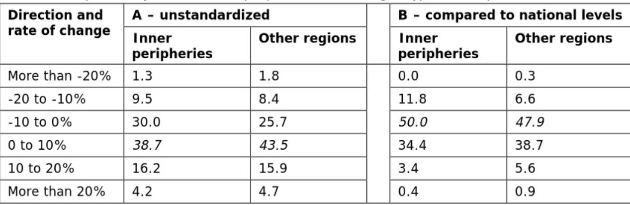
Table 4.2: Coverage of different types of inner peripheries by population dynamics trends (%) ... 112

Table 4.3: Migration paths in inner peripheral and other region types in Europe, 2000–2015 ... 113

Table 4.4: Coverage of different types of inner peripheries by migration trends (%) ... 116

Table 4.5: Coverage of different types of inner peripheries by ageing trends (%) ... 119

Table 4.6: Coverage of different types of inner peripheries by inactivity trends (%) ... 123

Table 4.7: Coverage of different types of inner peripheries by unemployment trends (%) ... 127

Table 4.8: Coverage of different types of inner peripheries by (low) qualification trends (%) 131 Table 4.9: Coverage of different types of inner peripheries by economic performance (GDP) trends (%) ... 135

Table 4.10: Coverage of different types of inner peripheries by employment trends in manufacturing industry (%) ... 139

Table 6.1: Variables of analysis ... 168

Table 6.2: Pseudo F values ... 170

Table 6.3: Characteristics of clusters (means) ... 171

Table 6.4: Cluster descriptions ... 172

Table 6.5 Summary statistics for Cluster 1 (N=179) ... 173

Table 6.6: Summary statistics for Cluster 2 (N=46) ... 173

Table 6.7: Summary statistics for Cluster 3 (N= 163) ... 174

Table 6.8: Summary statistics for Cluster 4 (N=127) ... 174

Table 6.9: Cluster membership at country level ... 176

(16)

Table 7.2: Comparison of distributions of old age dependency data (standardized as percentages of national averages) of inner peripheries and other regional typologies (p-value of Kolmogorov-Smirnov test) ... 187 Table 7.3: The correlation between IP coverage of NUTS 3 regions and socio-economic indicators (unstandardized) ... 190 Table 7.4: The correlation between IP coverage of NUTS 3 regions and socio-economic indicators (standardized as percentages of national averages) ... 191 Table 7.5: The correlation between IP coverage of NUTS 3 regions and socio-economic indicators (unstandardized), by the exclusion of centres (units with 0% share of inner peripheral areas)... 192 Table 7.6: The correlation between IP coverage of NUTS 3 regions and socio-economic indicators (standardized as percentages of national averages), by the exclusion of centres (units with 0% share of inner peripheral areas) ... 192

(17)

Abbreviations

<EU75% Lagging regions at European level, when GDP per capita was lower than 75% of the European average

<EUNAT75% Areas both lagging at European and national levels

<NAT75% Lagging at national level, when GDP per capita was lower than 75% of the national average

<OnlyEU75% Areas only lagging at European level

<OnlyNAT75% Areas only lagging at national level A–D Accumulating–Depleting

AT Austria

BE Belgium

Benelux Belgium, the Netherlands and Luxembourg

BG Bulgaria

CZ Czech Republic

DE Germany

DG Directorate-General

DG AGRI Directorate-General for Agriculture and Rural Development DG REGIO Directorate-General for Regional and Urban Policy

DK Denmark

EE Estonia

EC European Commission

EDORA European Development Opportunities in Rural Areas e.g. For example (in Latin)

EL Greece

ES Spain

ESPON European Observation Network for Territorial Development and Cohesion

EU European Union

F/M Female/Male

FI Finland

FR France

FYROM Former Yugoslavian Republic of Macedonia GDP Gross Domestic Product

GVA Gross value added

HR Croatia

HU Hungary

i.e. That is (in Latin)

IE Ireland

inh inhabitants

IP Inner periphery(ies)

ISCED International Standard Classification of Education

IT Italy

K-S test Kolmogorov-Smirnov test

LT Lithuania

LU Luxembourg

LV Latvia

Max. Maximum

Min. Minimum

(18)

PL Poland

PPS Purchasing Power Standard

PROFECY Processes Features and Cycles of Inner Peripheries in Europe

PT Portugal

QCA Qualitative comparative analysis R&D&I Research, Development and Innovation

RO Romania

SE Sweden

SEMIGRA Selective Migration and Unbalanced Sex Ratio in Rural Regions SGI Service(s) of General Interests

SI Slovenia

SK Slovakia

Std. Deviation Standard deviation U–R typology Urban-Rural typology

UK United Kingdom

UN United Nations

Y Yes

(19)

1 Introduction

1.1 Aims and tasks of analysis

In characterising inner peripherality a key objective is to place inner peripheries delineated by ESPON PROFECY project in the socio-economic space of Europe. The status of inner peripheries cannot be really understood and interpreted in itself, but by compared to other types of regions in Europe. Thus, during analyses implemented here, the main question was what made these territories differentiable from other areas in terms of geographical patterns and various socio-economic characteristics. Overlapping and differentiated geographies between inner peripheries and other types of regions might indicate how close they are to each other in a physical sense, and what aspects of spatiality form regional patterns of this image. The comparison of the socio-economic status of inner peripheral areas and other typologies might reveal if IP regions have entirely unique features or these are inseparable from characteristics and potential mechanisms affecting other regions with certain socio- economic or geographical specificities too.

Analyses are not only focused on positioning between IP and other areas in the ESPON space, but on exploring similarities and differences within the groups (different types) of inner peripheries too. It might help to resolve if inner peripheries identified by delineations framed by a multidimensional understanding of peripheralization form a group with common characteristics or they are rather different, with having different reasons to be peripheral.

Another important objective of characterising inner peripheries is to capture trends potentially affecting the socio-economic positions of inner peripheries. Besides following socio-economic tendencies and their regional patterns over time, it might also help to answer what makes IP to be evolved from the viewpoint of socio-economic factors.

These aspirations were translated into different tasks to be analysed whose findings are presented here in the Final Report:

• Providing an analysis on the geographies of European inner peripheries compared to other territories with certain geographic or socio-economic specificities;

• Analysing the socio-economic status of inner peripheries by exploring similarities and differences with other regional typologies;

• Following changes of socio-economic characteristics over time;

• Exploring the connection between the spatial dimension of centrality–peripherality at the European scale and different features reflecting on the social characteristics or economic performance of regions (and in particular inner peripheral areas);

• Analysing the status of inner peripheries, by characterising the regional and socio-

(20)

kept at this level to have a common basis in comparisons among different types of inner peripheral areas. Similar considerations were taken into account in the case of geographical and socio-economic comparisons between IP regions and other typologies (EU regional typologies, lagging areas), which are only available at this administrative level. On the other hand, realities of gathering comprehensive socio-economic information for a Europe-wide analysis on the status of inner peripheries also supported NUTS 3 level analyses. By being aware of potential drawbacks of identifying IP at this level, in characterising inner peripherality, several supplemental experiments are carried out for refining the interpretation of status of inner peripheries.

1.2 Database of research tasks

1.2.1 Selection of regional typologies used in the analysis

Among typologies available at NUTS 3 level in the NUTS 2013 system not all region types are used in the analysis built on the comparison of geographical patterns and socio-economic status of inner peripheries and other regions with geographical specificities or economic performance characteristics. The selection principles of typologies used served the goal of making the comparison of different datasets (IP regions and other areas) more meaningful for the research.

Several typologies for potential use include a large number of regions, covering even the third or more of the 1400–1500 NUTS 3 units considered. When analysing group specificities or distribution characteristics of these region types, it is hard to interpret them, because of the great variety of these areas, including more disadvantaged or more developed territories as well at the same time. On the contrary, a more limited number of regions within a typology category might show more significant and specific information on group characteristics.

In this way, from Urban-Rural typology of DG AGRI and DG REGIO, the category of

‘Intermediate’ regions are considered to be challenging to be interpreted, but was kept for these analyses (Table 1.1). This category consists of a large number of areas, which might be transitional in their socio-economic characteristics, not only by taking into account their geographical status between urban and rural regions. While ‘Urban’ and ‘Rural’ classes, however also contain numerous areas, they might show more specificities in this sense as separate groups. Similarly to intermediate regions, elements of Metropolitan region typology were also considered to be hard to interpret as a coherent groups. This typology covers metropolises and their hinterlands, consisting of urban, intermediate or rural regions too, with potentially very diverse socio-economic characteristics. Regarding these potential drawbacks and the strong similarity considering group characteristics with urban regions, metropolitan areas were excluded from some of the analyses.

(21)

Table 1.1: Selection of regional typologies used in analyses

Typology name Elements Source Used in

analyses Name in analyses Urban-Rural typology

DG AGRI and DG REGIO

Predominantly urban Yes Urban

Intermediate Yes

Predominantly rural Yes Rural

Typology on mountain areas

DG Regio

> 50 % of population

live in mountain areas No

> 50 % of surface are in

mountain areas No

> 50 % of population and > 50 % of surface

are in mountain areas Yes Mountain

Typology of NUTS 3 regions entirely composed of islands

DG Regio major island < 50,000

inhabitants

Yes (as joint

category) Island major island between

50,000 and 100,000 inh.

major island between 100,000 and 250,000 inh.

island with 250,000 - 1 million inhabitants island with >= 1 million inhabitants

Metropolitan region typology

DG Regio Capital metropolitan

region Yes (as joint

category) Metropolitan Metropolitan region

Typology of lagging regions

Own calculation GDP per capita (PPS) is

lower than 75% of EU28

average Yes Lagging

(<EU75%) GDP per capita (PPS) is

lower than 75% of EU28 average but not lower than 75% of national average

Yes Lagging

(<OnlyEU75%)

GDP per capita (PPS) is both lower than 75% of the national and EU28 averages

Yes Lagging

(<EUNAT75%) GDP per capita (PPS) is

lower than 75% of

national average but not Yes Lagging

(22)

From different categories of mountain area typology, only those areas were processed into the analyses, which covers regions with >50 % of population and >50 % of surface is in mountain areas. These criteria might ensure to be more focused when considering mountain region characteristics of distribution of population and economic activities, since they exclude those mountain areas where the majority of population resides in lower elevated areas.

Contrary to that, all categories of ‘Island’ typology are considered to be kept for the analysis, since several socio-economic specificities related to island positions (demographic characteristics, industries, accessibility conditions etc.) might affect this entire group independently from the size-factor, at least in some extent.

The definition of lagging areas is a relative and open issue, since it is not a fixed and permanent category and significantly depends on both the level of comparison (lagging compared to what, at what regional level) and the purpose of classification. In academic papers researchers might have more space to formulate and develop complex ways of identifying with a potentially better targeting ability. Complex and innovative options for defining lagging regions in European-level policy oriented researches, such as the classification of DG Internal Policies analysis¹ or the ESPON EDORA typology (A–D type)² provide interesting insights on how to define socio-economically disadvantaged areas without restricting it to one or two underlined aspects, and be comprehensive at the European level.

These experiments rarely build into actual policy practices. From the viewpoint of EU-level classifications, such methodologies are more favourited, which are reproducible, traceable and available (regarding data needs) for a continent-wide coverage. This might indicate the advantage of using simple indicators for policy purposes. Nevertheless, these can only have restricted facilities in interpreting disadvantages of regions in a complex way, so their connection to the phenomena to be identified should be clear for a reliable usage.

The European Commission use the simple GDP per inhabitant value-based classification in determining the eligibility of NUTS 2 regions for accessing EU Structural Funds (for lagging regions). It emphasises the role of economic performance in disadvantaged status of regions by implying that those areas might be lagging, which lack economic capacities to perform (better). This definition compares GDP/capita (PPS) values of regions to the EU average.^3,4. Three classes are formed by this method: less developed (GDP/capita < 75% of EU average), transition (GDP/capita = 75–90% of EU average), more developed (GDP/capita > 90% of EU average).

The categorisation provides an acknowledged and well-grounded regional typology of economic performance, and is selected to be used in analyses of ESPON PROFECY project for identifying lagging areas. Nevertheless, some drawbacks affect this mode of defining lagging regions that one needs to have in sight. These shortcomings of this categorisation might be overcome by different ways of fine tuning. Current categorisation of NUTS 2 regions eligible for subsidy can be updated by the most recent data on regional performance

(23)

(GDP/capita), which is based on three years average values (most current data cover years 2013–2015).

It is also possible to keep the criterion of ‘GDP/capita below 75% of EU average’ as a form of identification of less developed regions, but do the calculations directly at NUTS 3 level. This might have an impact on the accuracy of targeting, since many NUTS 2 regions consist of different types of areas regarding economic performance, which might cover the presence of several disadvantaged areas, while identifying others which are less affected by these handicaps.

Another option for fine tuning this methodology might be using the ‘below 75%’ criterion not just by comparing regional performance values to the EU average, but reflecting on within country differences too. From policy-oriented aspects, this option might gain importance, since it puts emphasis not only on lagging regions measured at the European level, but the presence of territorial inequalities at national levels too. On the one hand, it might represent multiply disadvantaged regions by the coincidence of certain degrees of deviation both from EU and national average, on the other hand, it helps to fine tune this type of measure to outline areas identified as lagging in national context in more developed countries.

Figure 1.1: Lagging region typologies used in ESPON PROFECY project

During the identification of lagging areas (for comparing them to the status of inner peripheries) in PROFECY analyses these options were taken into consideration.

(24)

regions, whose GDP per capita value do not reach the 75% of EU28 average but their economic performance is above the 75% level of their national average. Another group consists of the less developed regions in the comparison, lagging behind the 75% of both the EU and national GDP per capita averages. While the last two groups of lagging areas cover those regions, which were identified as disadvantaged by considering their GDP per inhabitant level compared to national averages (including disadvantaged areas at the EU level too) or only regarding their GDP per inhabitant level compared to national averages. In some parts of the analyses joint categories representing all regions lagging in the EU context or outlining every economically disadvantaged area from national aspects are not listed (see for instance Chapter 3).

1.2.2 Presentation of socio-economic data used

In the investigations of socio-economic characteristics of inner peripheries, a multiple indicator-based way of analysis was chosen. By covering several dimensions potentially connected to the status of inner peripheral areas compared to other region types as state parameters, a balanced insight on their socio-economic specificities are intended to be interpreted. The selection of indicators to be used needed to take attention to several aspects for composing a meaningful analysis.

One of the main questions related to the analysis of status of inner peripheries is if (and how) socio-economic characteristics of the delineated IP areas could be traced back to their special socio-spatial conditions. Basic structures of processes leading to the evolution of inner peripheries were already outlined by the Inception and Interim Reports of ESPON PROFECY project^5,6. Assumptions related to the interpretive and descriptive models of different conceptual types of inner peripherality highlighted potential causes and drivers of peripheralization and also underlined various socio-economic consequences associated with the phenomena.

By the analysis of these consequences, broader problem areas related to different conditions and processes associated with demography, social capital, economic performance, and the availability of services of general interests were defined. And within these domains dimensions with narrower meaning were also named. For filling up these dimensions with content, quantifiable indicators were assigned to them, from the database gathered before, mainly from Eurostat sources at NUTS 3 level.

Potential demographic problems of inner peripheries (and other region types) are illustrated by indicators of consequences of depopulation and outmigration tendencies (population change, migration rate, ratio of child age and active age population etc.) and measures related to disadvantaged demographic conditions, such as ageing (old age dependency rate), gender imbalances (gender balance of working age population) or poor health conditions (crude death rate) (Table 1.2).

(25)

Table 1.2: The structure and selection of indicators for analyses

Problem areas Dimensions Indicators Used in

ansalyes?

Demographic problems and disadvantaged demographic conditions

Outmigration of young active population

Population change, % Y

Migration rate, % Y

Migration rate of active age

population (15–64), % N

Ratio of child age population (0–14),

% Y

Ratio of young age population (15–

24), % N

Ratio of working age population (15–

64), % Y

Disadvantaged demographic composition and processes

Old age dependency rate, % Y Gender balance (F/M) of working

age (15–64) population, % (Y)

Crude birth rate, % N

Crude death rate, % (Y)

Decline of social capital

Low labour market participation

Inactivity rate (15+), % Y Gender gap in activity (F/M), % Y Unemployment rate (15+), % Y Youth unemployment rate (15–24),

% N

Long-term unemployment rate

(15+), % N

NEET rate (15–24), % (Y)

Low qualification

Ratio of population with low qualification (ISCED 11 0–2) (25–

64), % Y

Ratio of population with high qualification (ISCED 11 5–8) (25–

64), % N

Low economic potential

Low productivity

GDP (PPS) per inhabitant, %

EU28=100 Y

GVA per inhabitant, Thousand € N GVA per employed persons,

Thousand € Y

Ratio of employed persons in

agriculture (NACE_rev2 A), % N Ratio of employed persons in

manufacturing (NACE_rev2 C), % Y

Low entrepreneurship and innovation

Number of active enterprises per

10000 persons Y

Birth rate of enterprises, % Y Death rate of enterprises, % N

(26)

Problem areas Dimensions Indicators Used in ansalyes?

persons

Density of pharmacies, per 10000

persons N

Density of primary schools, per

10000 persons Y

Density of secondary schools, per

10000 persons N

Density of retail units, per 10000

persons Y

Maximum and average travel times

to SGI units, minute Y

The potential decline of social capital is measured by different participation rates at the labour market (for example, inactivity, unemployment, gender gap, NEET) and educational attainment data representing qualification characteristics. Economic potentials of the analysed areas and groups of regions are illustrated by productivity indicators such as GDP per inhabitants of GVA per employed persons or the ratio of employed persons in manufacturing industry. Furthermore, the dimension of entrepreneurship is also covered by different business demography measures (number of active enterprises, birth rate, survival rate of enterprises) – but only for a group of available countries.

As measures of consequences of poor provision of services of general interests, indicators reflecting on the availability and density of SGI are also built in the analysis, by representing service sectors of health, education and retail. In some analyses maximum or average travel time to these SGI units were also used as indicators.

Because of the big number of variables covering similar data topics, a pre-selection of these measures was implemented for further use. Correlation analyses among indicators of the same dimensions were carried out, and based on statistical correlations and the known logical relationships between variables a part of these indicators was excluded from accomplished analysis. Only the ones, thought to be the most representative were processed into further investigations.

1.2.3 Processing territorial units into analyses

Goals and methodologies of different tasks during the analysis of status of inner peripheries determine, how the four different delineated types of inner peripheries be made enter common analyses. Although most of the presented methods are suitable for representing different types of regions identified as inner peripheries separately, it might multiply elements of tools of visualisation and analysis. Because of that, in some cases it is proposed to make the ‘union’ of different types of IP enter the analyses (Figure 1.2). In this way, the project group could work with the widest pool of IP regions, while the differentiation between types of inner peripheries should be taken into account when choosing the focus of interpretation of results. This could be adequate in those cases, where individual NUTS 3 units are basic

(27)

elements of analysis (e.g. time-series analysis – Chapter 4 –, scatter plot analyses – Chapter 5 – and cluster analysis-based socio-economic classification of IP – Chapter 6). Where these basic elements are groups of regions (e.g. in comparisons of the overlap between IP and other region types – Chapter 2 – or in tasks using box plots Chapter 3 and Chapter 5), keeping the separation of different IP types seems to be more adequate.

Figure 1.2: Inner peripheries counted by different types and by the ‘union’ of different delineations

Region IP Type1 IP Type2 IP Type3 IP Type4 IP count Region IP?

A 1 0 0 0 1 A Y

B 0 0 0 0 0 C Y

C 0 0 1 0 1 D Y

D 1 0 0 0 1 G Y

E 0 0 0 0 0 I Y

F 0 0 0 0 0 K Y

G 1 1 1 1 4 L Y

H 0 0 0 0 0 N Y

I 0 1 0 0 1 Q Y

J 0 0 0 0 0 S Y

K 0 0 1 0 1 U Y

L 1 0 0 1 2 W Y

M 0 0 0 0 0 Y Y

N 0 1 0 0 1 Z Y

O 0 0 0 0 0

P 0 0 0 0 0

Q 0 0 1 0 1

R 0 0 0 0 0

S 1 0 1 0 2

T 0 0 0 0 0

U 0 1 0 1 2

V 0 0 0 0 0

W 0 0 0 1 1

X 0 0 0 0 0

Y 0 0 1 0 1

Z 1 0 0 0 1

(IP types and region labels listed in the figure above are not actual results from the projects. These are just hypothetical examples for demonstrating principles of counting of areas identified as inner

peripheries by separating the different cases of delineations or by using a merged pool of all types, which determines how to process territorial units into analyses.)

1.3 Inner peripheries and areas at risk of becoming peripheral

Besides the delineation of the four groups of inner peripheries, ESPON PROFECY project made experiments and recommendations for identifying territories at risk of becoming inner peripheral as well. These ideas can be found in Chapter 4.3 in the Final Report and in the form of a more detailed version in Chapter 5 in Annex 4 for the Final Report. Areas identified as territories at risk of becoming inner peripheries are not proceeded into analyses related to tasks characterising the status of inner peripheries in Europe due to several considerations.

(28)

peripheries, the situation would presumably be very complicated. The four groups of inner peripheries themselves have different combinations of overlaps, what raises challenges in the interpretation of their socio-economic characteristics, and determines how they can be proceeded into analyses (see previous Chapter 1.2.3). These issues are managed in different ways in analyses presented in this report. But with a potential addition of a further dimension of territorial units to be analysed, too many combinations would occur, which would be difficult to be filled with meaningful content in terms of ‘actual’ socio-economic phenomena.

Approaches of delineating territories at risk of becoming inner peripheral presented in Chapter 5 in Annex 4 for the Final Report provide options for the identification of these areas of risk on the basis of their potential dependence on one SGI facility or their multiple, but not critical disadvantages regarding access to different services at grid level. NUTS 3 level assignment of these territories is not carried out, because these areas are usually comparatively small and by being scattered across the countries they do not form continuous patches. In this way, these territorial units would hardly fit into the framework of methodologies used and data needs fulfilled for analysing the status of areas associated with phenomena of inner peripherality. Even if data supply regarding these units could practically be satisfied, it would be difficult to match meaningful variables to the description of them, because potential risks of peripheralization from the viewpoint of SGI access might not always have direct links to socio- economic trends, since e.g. in the provision of services, administrative or political motives are also present.

Analyses presented in the report aim at exploring territorial and socio-economic specificities of inner peripheral areas, in most of the introduced tasks in comparison with other European region types (what kind of socio-economic challenges affects them, is their status less or more disadvantaged compared to other typologies etc.). Despite previous explanations, the position of regions of risk might potentially be derived indirectly from findings of these analyses. Identified vulnerabilities, unfavourable socio-economic conditions associated with inner peripheries might be considered as potential risk factors in processes of peripheralization. If non-peripheral areas share these vulnerabilities or have specific combinations of them, it might indicate dangers of becoming inner peripheries. It might happen in the case, if their opportunities of access or position regarding connectedness deteriorate, which could cause higher risks than in the case of actual IPs with less disadvantaged socio-economic position.

(29)

2 Analysing geographies of European inner peripheries compared to regional typologies on other territorial realities

2.1 Overlap between inner peripheries and EU regional typologies

The analysis based on the comparison of deviations and overlaps between geographies of IPs and other regional typologies in Europe is using cross table analysis and overlaid maps to gain information on meaningful patterns. Units of analyses are provided by the delineation process identifying four groups of inner peripheral areas. Besides, regional typologies widely used in association with NUTS 3 EU regions (separated elements of Urban–Rural typology, mountain areas, islands and metropolitan regions) are also processed into analyses. Since a special focus on lagging areas is expected to be applied in comparisons with inner peripheries, different groups of lagging EU regions are identified by economic performance (GDP per inhabitant) in relation to EU and national averages.

Results based on cross tables and overlaid maps indicate significant overlap between different groups of inner peripheries and other regional typologies. In general, regarding EU regional typologies, inner peripheral regions most frequently tend to overlap with intermediate regions (Map 2.1–Map 2.4), rural regions (Map 2.5–Map 2.8) and mountain areas (Map 2.13–

Map 2.16) (see also Table 2.1). Besides, other regional types might show more notable overlap with one or another IP delineation types, such as in the case of depleting inner peripheries and urban areas (Map 2.9–Map 2.12) or metropolitan areas, which imply that processes of marginalisation could significantly affect these territories too.

Table 2.1 shows the overlap between IP regions (resulting from the four delineations) and other regional typologies for Europe. Regarding IP delineations 1 and 3 (based in lower accessibility to regional centres and SGIs) it is worth mentioning that around half of them are identified as mountain regions. By contrast, the overlapping percentage is lower for mountain areas regarding IP Delineation 2 (lower economic potential interstitial areas), and Delineation 4 (depleting areas). This overlap is mostly located in the biggest mountain ranges. It should be noted that mountains have a major influence reducing accessibility due to geographical factors, therefore they also influence the averaging process used to delineate IPs.

Notwithstanding that, there are also inner peripheries in less mountainous areas.

Regarding the urban-rural typology it is interesting to note that most IP regions are located in non-urban areas (>80%), except for Delineation 4 (depleting areas) where IPs are distributed more or less equally between the three categories (urban, intermediate, rural). However,

(30)

Table 2.1: Overlap between inner peripheries and EU regional typologies Urban

regions Intermediate

regions Rural

regions Mountain

regions Island

regions Metropolitan regions IP 1 (regional

centres) 9.6% 48.6% 41.8% 49.5% 0.0% 24.0%

IP 2

(interstitial) 18.8% 40.0% 41.2% 38.2% 1.2% 23.0%

IP 3 (SGI

access) 10.8% 44.1% 45.2% 53.8% 1.1% 20.4%

IP 4

(depleting) 32.2% 34.1% 33.7% 24.4% 2.6% 43.0%

The following tables present an analysis of the overlap between inner peripheries and EU regional typologies for the different macro-regions in Europe (countries are grouped according to its geographical location based on the Eurovoc Classification^a). The text below presents the results of the overlap of the four Delineations for Central and Eastern Europe (Table 2.2);

Western Europe (Table 2.3); Southern Europe (Table 2.4) and Northern Europe (In Southern Europe (Table 2.4) it is remarkable the high proportion of IPs located in intermediate regions (ranging from 39% to 70% of IPs). However, for Delineation 4 the number of IPs located in rural regions is more relevant. In this macro-region, the presence of mountainous regions seems very relevant and it is related to the existence of IPs, as there is a high percentage of IPs located in these areas (ranging from 58 to 88% depending on the Delineation).

In Northern Europe (Table 2.5), IPs are mostly located in non-urban regions (only showing a slight overlap in Delineation 1). In addition, depending on the delineation used, they mostly overlap with rural regions (Delineation 1, 2 and 4) or with intermediate ones (Delineation 3).

Delineation 4 also shows an important overlap (>45%) with the intermediate typology of regions. The overlap between mountain regions and the different four delineations shows also and interesting results, as there is a relevant overlap with delineations 1 (38%) and 2 (43%) while the overlap is low or inexistent for the other two delineations.

Table 2.5).

a Eurovoc Classification: Central and Eastern Europe (Albania; Belarus; Bosnia and Herzegovina;

Bulgaria; Croatia; Czech Republic; Former Yugoslav Republic of Macedonia; Hungary; Kosovo;

Moldova; Montenegro; Poland; Romania; Russia; Serbia; Slovakia; Slovenia; and Ukraine; where Turkey has also been added); Western Europe (Andorra; Austria; Belgium; France; Germany; Ireland;

Liechtenstein; Luxembourg; Monaco; Netherlands; Switzerland; and United Kingdom); Southern Europe (Cyprus; Greece; Italy; Malta; Portugal; San Marino; and Spain) and Northern Europe (Denmark; Estonia; Finland; Iceland; Latvia; Lithuania Norway; and Sweden).

(http://eurovoc.europa.eu/drupal/?q=request&view=mt&mturi=http://eurovoc.europa.eu/100277&languag e=en)

(31)

Table 2.2: Overlap between inner peripheries and EU regional typologies (Central and Eastern Europe) Urban

centres) 7.0% 39.5% 53.5% 48.8% 0.0% 11.6%

IP 2

(interstitial) 6.7% 37.8% 55.6% 55.6% 0.0% 8.9%

IP 3 (SGI

access) 0.0% 46.2% 53.8% 76.9% 0.0% 0.0%

IP 4

(depleting) 11.1% 25.9% 63.0% 59.3% 0.0% 18.5%

In Central and Eastern Europe (Table 2.2) IPs overlap less with urban regions, as about 90%

of IPs are located on the other categories of the urban-rural typology. In addition, the percentage of IPs in Mountain regions is significantly high (>50%) for all the delineations, being particularly high (>75%) regarding Delineation 3, based on access to SGIs. As these countries are located inland, and subsequently there are no IPs on Island regions. On the other hand, the overlap of IPs with metropolitan regions is low (10%), although the value doubles for Delineation 4.

Table 2.3: Overlap between inner peripheries and EU regional typologies (Western Europe) Urban

centres) 11.2% 48.0% 40.8% 40.8% 0.0% 33.7%

IP 2

(interstitial) 28.8% 42.5% 28.8% 15.0% 0.0% 35.0%

IP 3 (SGI

access) 15.0% 35.0% 50.0% 41.7% 0.0% 28.3%

IP 4

(depleting) 41.9% 33.3% 24.7% 11.8% 2.2% 56.5%

In Western Europe (Table 2.3) most of the IPs are not located intermediate and rural regions, with the exception of Delineation 4 where the overlap of IPs and urban areas increases until 29%. The IPs of Western European countries in Mountain regions varies significantly depending on the delineation used: if the focus is set on the distance to regional centres or SGIs (Delineation 1 and 3) the number of IPs is approximately three times than for Delineation 2 (lower economic potential interstitial areas) and 4 (depleting areas). Regarding metropolitan regions, a relevant proportion of IPs in can be observed for all delineations, where again Delineation 4 stands out (>50%).