Ecological Indicators 127 (2021) 107752
Available online 4 May 2021
1470-160X/© 2021 The Authors. Published by Elsevier Ltd. This is an open access article under the CC BY-NC-ND license
(http://creativecommons.org/licenses/by-nc-nd/4.0/).
Quantifying 3D vegetation structure in wetlands using differently measured airborne laser scanning data
Zs ´ ofia Koma
a,*, Andr ´ as Zlinszky
b, L ´ aszl ´ o Bek ˝ o
c, P ´ eter Burai
c, Arie C. Seijmonsbergen
a, W.
Daniel Kissling
a,daInstitute for Biodiversity and Ecosystem Dynamics (IBED), University of Amsterdam, P.O. Box 94240, 1090 GE Amsterdam, The Netherlands
bBalaton Limnological Institute, Centre for Ecological Research, Hungarian Academy of Science, Klebelsberg Kuno út 3, 8237 Tihany, Hungary
cRemote Sensing Centre, University of Debrecen, B¨osz¨orm´enyi Road 138, 4032 Debrecen, Hungary
dLifeWatch Virtual Laboratory Innovation Center (VLIC), LifeWatch ERIC, P.O. Box 94240, 1090 GE Amsterdam, The Netherlands
A R T I C L E I N F O Keywords:
Full waveform ALS Discrete return ALS Marshlands Reedbeds Biomass LAI Height
A B S T R A C T
Mapping and quantifying 3D vegetation structure is essential for assessing and monitoring ecosystem structure and function within wetlands. Airborne Laser Scanning (ALS) is a promising data source for developing in- dicators of 3D vegetation structure, but derived metrics are often not compared with 3D structural field mea- surements and the acquisition of ALS data is rarely standardized across different remote sensing surveys. Here, we compare a set of Light Detection And Ranging (LiDAR) metrics derived from ALS datasets with varying characteristics to a standardized set of field measurements of vegetation height, biomass and Leaf Area Index (LAI) across three Hungarian lakes (Lake Balaton, Lake Fert˝o and Lake Tisza). The ALS datasets differed in whether the recording type was full waveform (FWF) or discrete return, and in their point density (4 pt/m2 and 21 pt/m2). A total of eight LiDAR metrics captured radiometric information as well as descriptors of vegetation cover, height and vertical variability. Multivariate regression models with field-based measurements of vege- tation height, biomass or LAI as response variable and LiDAR metrics as predictors showed major differences between ALS recording types, and were affected by differences in spatial resolution, temporal offset and sea- sonality between field and ALS data acquisition. Vegetation height could be estimated with high to intermediate accuracy (FWF ALS data only: R2 =0.84; combination of ALS datasets: R2 =0.67), demonstrating its potential as a robust indicator of 3D vegetation structure across different ALS datasets. In contrast, the estimation of biomass and LAI in these wetlands was sensitive to variation in ALS characteristics and to the discrepancies between field and ALS data in terms of spatial resolution, temporal offset and seasonality (biomass: R2 =0.20–0.22; LAI:
R2 =0.08–0.30). We recommend the use of FWF ALS data within wetlands because it captures more vegetation structural details in dense reed and marshland vegetation. We further suggest that ecologists and remote sensing scientist should better coordinate the simultaneous and standardized acquisition of field and ALS data for testing the robustness of quantitative descriptors of vegetation cover, height and vertical variability within wetlands.
This is important for establishing operational and spatially contiguous ALS-based indicators of 3D ecosystem structure across wetlands.
1. Introduction
The physical structure of vegetation has a substantial influence on ecosystem productivity and on the availability of various carbon sources (Hall et al., 2011). Moreover, complex vegetation structure provides a greater volume of niche space available for species and thus enhances species richness (Moeslund et al., 2019). Hence, detailed quantification of vegetation structure is of key importance for biodiversity monitoring
and for assessing the structure and functioning of wetland ecosystems.
The time- and cost-efficient sampling of field measurements and the development of robust indicators for detecting and reporting changes in vegetation structure over broad spatial extents is an ongoing challenge for ecology (Pereira et al., 2013). Field measurements typically rely on manual methods and are locally restricted, e.g. being measured within vegetation plots (Hyypp¨a et al., 2008; Cao et al., 2014; Luo et al., 2015;
Moeslund et al., 2019). Manual methods of measuring vegetation
* Corresponding author.
Contents lists available at ScienceDirect
Ecological Indicators
journal homepage: www.elsevier.com/locate/ecolind
https://doi.org/10.1016/j.ecolind.2021.107752
Received 15 January 2021; Received in revised form 8 April 2021; Accepted 21 April 2021
structure can be non-destructive, e.g. for measuring vegetation height (Hopkinson et al., 2004; Luo et al., 2015; Nie et al., 2018), or destruc- tive, e.g. by harvesting above-ground vegetation to estimate plant biomass (Fliervoet and Werger, 1984; Mitchley and Willems, 1995).
Some vegetation structural parameters such as the Leaf Area Index (LAI) and estimates of vegetation cover can be obtained by using digital methods such as hemispherical (Jonckheere et al., 2004) or classical photography (Liu and Pattey, 2010). Direct field measurements are considered to be the most precise methods, but obtaining vegetation structural parameters in the field is labor-intensive, time-consuming, and expensive and thus limited in spatial extent, typically to a few study sites. Moreover, areal field surveys in some wetland vegetation types (e.
g. flooded plains) are particularly difficult. The development of quan- titative, accurate, and standardized indicators of vegetation structure over broad spatial extents therefore requires additional approaches such as indirect remote sensing methods (Serbin and Townsend, 2020).
Remotely sensed data such as Light Detection and Ranging (LiDAR) show great potential for estimating vegetation structural parameters in a spatially contiguous way (Lefsky et al., 2002; Davies and Asner, 2014;
Moeslund et al., 2019). Particularly, Airborne Laser Scanning (ALS) is becoming increasingly available over large spatial extents (Valbuena et al., 2020). ALS measurements use the time difference between a laser pulse emitted from an airborne sensor and the return signal from the vegetation (leaves, branches stems) or the ground. Based on the returned signal the x,y,z coordinates of the objects can be calculated, resulting in a 3D point cloud capturing objects and the ground. Besides recording the coordinates of each surveyed laser return point, the intensity of the re- flected light energy is additionally recorded. The ALS quality of the measured dataset can vary depending on the sensor type and the ALS data acquisition parameters (e.g. flight height, pulse rate frequency, scan angle and footprint) (Shan and Toth, 2018). Most commercial ALS systems deliver discrete return (DR) point cloud data (Ussyshkin and Theriault, 2011) which record multiple returns per laser pulse (typically 1–5 saved echoes). In contrast, full waveform (FWF) LiDAR sensors digitize the total amount of laser energy returned to the sensor in fixed time intervals (1–5 ns) and thus provide a near continuous distribution of backscattered laser intensity for each recorded pulse (Mallet and Bretar, 2009). To derive ecologically relevant indicators, the 3D point clouds need to be further processed, e.g. into LiDAR metrics which statistically aggregate the 3D point cloud information within spatial units such as raster cells (Bakx et al., 2019; Davies and Asner, 2014;
Meijer et al., 2020). These LiDAR metrics can quantify vegetation height (e.g. maximum z values within a cell) or vertical variability of the vegetation structure (e.g. variance of z within a cell). LiDAR metrics together with in-situ collected field inventory data enable to quantify vegetation height (Hopkinson et al., 2004, 2006; Nie et al., 2018), biomass (Hyypp¨a et al., 2008; Cao et al., 2014) and LAI or vegetation density (Luo et al., 2015; Koma et al., 2018). While the development of indicators related to vegetation structure derived from ALS data has received a lot of attention in forest ecosystems (Maltamo et al., 2014), little attention has yet been given to low-stature ecosystems with pre- dominantly herbaceous vegetation.
In the context of wetlands, the use of ALS data for quantifying vegetation structure has mostly focused on mapping ecosystem extent or on classifying different types of wetland vegetation (Zlinszky et al., 2012; Millard and Richardson, 2013; Chasmer et al., 2016; Koma et al., 2021). Only a few studies have yet established statistical relationships between in-situ field measurements of the 3D vegetation structure and ALS-derived LiDAR metrics within wetlands. For example, vegetation height was estimated within reedbeds of specific lakes in Canada, En- gland and China, using the standard deviation or the 99th percentile of z (T¨oyr¨a et al., 2003; Onojeghuo and Blackburn, 2013; Nie et al., 2018).
Similarly, vegetation biomass has been estimated from height-related metrics (99th of percentile of z) combined with hyperspectral (Luo et al., 2017) or other optical remote sensing products (Riegel et al., 2013). One study investigated the estimation of LAI (Luo et al., 2015)
and showed that vegetation height and the pulse penetration ratio (a metric reflecting vegetation openness) are important LiDAR-based pre- dictor variables. These previous studies have focused on specific wetland sites to optimize the statistical relationships between field measure- ments and ALS derived metrics, e.g. by maximizing the explained vari- ance (R2) or minimizing the root mean square error (RMSE). As a result, various site-specific relations for extracting vegetation structural pa- rameters in wetlands have been proposed, but it remains largely un- known whether such relationships are transferable to other wetland ecosystems and ALS data acquisition parameters.
The nation-wide ALS datasets often come with different character- istics (e.g. FWF versus DR, or with different point densities), and the simultaneous collection of field data is often infeasible (Koma et al., 2021). Additionally, the ALS flight campaigns are rarely done every year, despite decreasing operational costs. The use of DR data for the detection of low vegetation is also challenging because subsequent returns are too short or have too low intensity to be detected (Naye- gandhi et al., 2006; Hladik and Alber, 2012; Korpela et al., 2012; Shan and Toth, 2018). In contrast, FWF data acquisition can provide higher quality data (Mallet and Bretar, 2009), but the effect of the recording types of ALS data on estimating vegetation structural parameters within wetlands has not yet been tested. The variation of point densities across ALS datasets can further influence the statistical relationships between field measurements and ALS-based metrics: high point densities tend to provide accurate estimations of vegetation height, but low point den- sities and large illuminated footprints have limitations to penetrate through dense vegetation to the ground (Hopkinson et al., 2005; Luo et al., 2015; Hladik and Alber, 2012; Onojeghuo and Blackburn, 2013;
Nie et al., 2018). Moreover, ALS sensors are able to capture the ampli- tude (or intensity) typically in the infrared wavelength, but this attribute is usually omitted from further data analysis because information for applying radiometric calibration is often lacking (H¨ofle and Pfeifer, 2007). Further issues arise from the seasonality in vegetation growth and the temporal offset between the ALS acquisition (often during autumn, winter or spring) and the collection of in-situ field measure- ments (often in summer). Even though these practical and technical restrictions have been recognized in several case studies (Hopkinson et al., 2005; Hladik and Alber, 2012; Nie et al., 2018), no study has yet analyzed how ALS datasets with different qualities could be used to robustly estimate indicators of vegetation structure across wetlands.
Here, we statistically relate ALS datasets with different qualities to a standardized set of field measurements of vegetation structure (height, biomass and LAI) within wetlands. We focus on three Hungarian lakes with their emergent wetland macrophytes, including the common reed (Phragmites australis), bulrushes (Typha spec.) and sedges (Carex spec.).
The ALS data acquisitions for each lake have been measured in different years and with various flight survey specifications. The point densities therefore vary between 4 pt/m2 and 21 pt/m2 and either include DR or FWF data. Additionally, we manually measured different types of vegetation structural parameters in the field with a standard set of destructive, non-destructive, and imaging methods. Using these different ALS datasets and field measurements we (1) developed multivariate regression models to quantify vegetation height, biomass and LAI using LiDAR metrics derived at different spatial resolutions, and (2) analyzed how the characteristics of ALS data and the discrepancies between field and ALS data (spatial resolution, temporal offset and seasonality) affect the quantification of 3D ecosystem structure.
2. Material and methods
Our study has three main routines for the processing and analysis of in-situ field data in relation to the ALS datasets (Fig. S1): 1) collection, measurement and processing of field data, 2) processing of the different ALS datasets, and 3) analysis of the statistical relations between the field and ALS data. The ALS data processing and LiDAR metrics calculation were carried out using the LidR package (Roussel et al., 2020). The
scripts used in the processing and analysis are available from https://gi thub.com/komazsofi/PhDPaper3_wetlandstr.
2.1. Study area
The study area comprises three selected lakes in Hungary (Fig. 1).
Lake Fert˝o is a steppe lake located at the Austrian-Hungarian border and covers 315 km2. The water level is very sensitive to short-term climate variations due to its shallow depth and small catchment area. Lake Tisza is an artificial lake in the eastern part of Hungary. The lake covers 127 km2 and was created by damming of the Tisza River. Lake Balaton, located in the western part of Hungary, is the largest lake in Central Europe and covers 594 km2 area. More than half of the shoreline consists of reed-dominated wetlands.
2.2. Field data collection
The field measurements were acquired during the 2016 and 2017 summer months (June, July and August) across the three lakes (Fig. 1).
Individual sample plots were located along 26 transects from the lake side to the reedbed interior. Fourteen transects were sampled at Lake Ferto, five at Lake Tisza and seven at Lake Balaton, accessed with kayak ˝ in deeper water and by wading whenever water depth allowed. Within the transects two different types of field data were collected: i) plot-
based and ii) point-based measurements. Plot-based sampling was done with seventeen, six and eleven plots at Lake Fert˝o, Lake Tisza and Lake Balaton, respectively. A total of 253 point-based measurements were taken, 123 at Lake Ferto, 54 at Lake Tisza and 76 at Lake Balaton. ˝ Plot-based measurements were obtained within 0.5 m × 0.5 m quadrats, with the exact outlines being recorded by a Real Time Kine- matic Global Positioning System (RTK GPS). First, all reed vegetation within the quadrats was harvested. Second, the vegetation height in 50 cm intervals was measured using the GPS antenna pole (if the vegetation was taller than 2 m the pole base was lifted to continue measuring). Biomass was directly measured in the field as the total weight of the harvested above-ground vegetation parts (including fresh stalks and leaves as well as dry vegetation). The LAI measurements were carried out using a digital camera with a fixed focus. The digital photos were taken at ground or water level in a zenith-facing setup and were processed using the Green Crop Tracker software (Liu and Pattey, 2010).
2.3. Acquisition and processing of airborne laser scanning data
The ALS data were collected from four data acquisition campaigns (Table S1) and had different data characteristics. At Lake Balaton, DR data were captured in April 2014, with an average point density of 4 pt/
m2. The ALS point clouds for Lake Fert˝o were acquired in 2011 in the leaf off season (December), using a FWF sensor and an average point
Fig. 1. Study areas and sampling design at three Hungarian lake shores (A: Lake Balaton, B: Lake Fert˝o/Neusiedlersee, C: Lake Tisza). Red points indicate point-based measurements of Leaf Area Index (LAI) along transects. Yellow squares indicate plots (0.5 m ×0.5 m) in which biomass and vegetation height was measured. The background map is derived from Google Earth Imagery data. The maps are in the Universal Transverse Mercator (UTM) coordinate system zone 33 and 34. The overview map in the upper right shows the locations of A–C within Hungary. (For interpretation of the references to colour in this figure legend, the reader is referred to the web version of this article.)
density of 4 pt/m2. Lake Tisza was surveyed in FWF mode both in the leaf-off season (March 2012) and the leaf-on season (June 2013). The average point density was 21 pt/m2 and 18 pt/m2, respectively. All ALS data were measured in the infra-red wavelength (1064 nm for Lake Balaton, 1550 nm for the other sites). For surveys at Lake Ferto and Lake ˝ Tisza, a Riegl sensor (http://www.riegl.com/) was used, whereas at Lake Balaton a Leica sensor (https://leica-geosystems.com/) was used.
In a pre-processing step, we spatially selected the ALS point clouds using a 25 m radius around each field observation point (centroid of the quadrat). We then classified the selected points into ground and vege- tation using the Progressive Morphological Filter method (Zhang et al., 2003). To estimate the absolute (normalized) height of the vegetation points, the classified point cloud was normalized by subtracting the minimum height within 20 m grid cells from the ALS points. This normalization method is advantageous in wetlands (Zlinszky et al., 2012) to avoid errors in height calculations if no ground points are found below the reed canopy.
We calculated eight LiDAR metrics (Table 1) at three different spatial resolutions (0.5 m, 2.5 m, and 5 m radius around the field data points). If no ALS points were retrieved within the search radius around a field observation point, the field observation point was removed from further statistical analysis. We categorized the eight derived LiDAR metrics into four different feature classes (radiometric information, vegetation openness, vegetation height, and vertical variability). The radiometric information was not radiometrically calibrated since the flight trajec- tories were unavailable for the ALS datasets. The LiDAR metrics were identified from the literature based on their relevance for extracting vegetation height, biomass and LAI as well as our understanding of the physics of the LiDAR measurement process.
2.4. Statistical analysis
All LiDAR metrics were scaled by dividing the mean LiDAR metric by their standard deviations. We then analyzed the statistical relationship between the derived LiDAR metrics and the field measurements. First, a collinearity analysis among the derived LiDAR metrics was carried out using Spearman’s Rank correlations (r) (Fig. S2). We excluded variables that were highly correlated (r >0.6) to avoid multicollinearity between pairs of predictor variables (Moeslund et al., 2019). We then fitted multivariate linear regression models at three spatial resolutions (0.5 m, 2.5 m and 5 m) using vegetation height, biomass or LAI as response variables. We applied a backward variable selection based on the Akaike Information Criterion (AIC) to identify the most parsimonious model with a minimum set of predictor variables. We fitted models using either all field data collected across lakes (Lake Balaton, Lake Fert˝o and Lake Tisza) or using only FWF data (Lake Fert˝o and Lake Tisza). For LAI estimation, we additionally fitted separate models for each lake, and for Lake Tisza separate models for ALS datasets from March (leaf-off) and from June (leaf-on), respectively. We then compared the models be- tween the ALS data characteristics and spatial resolutions using
explained variance (R2), adjusted R-squared (adjusted R2) and Residual Standard Error (RSE). We further visualized the predicted and observed crossplots and partial dependence plots for the most important re- lationships in the multivariate linear regression models (as identified by standardized coefficients). These plots were then used for analyzing the effects of different ALS data characteristics and the discrepancies in spatial resolution, temporal offset and seasonality between field and ALS datasets.
3. Results
After the collinearity analysis, three LiDAR metrics were used as predictor variables for the multivariate linear regression models: i) the 99th percentile of height (H_p99), ii) the pulse penetration ratio (C_ppr), and iii) the standard deviation of the amplitude (A_std). We present the most parsimonious models based on an Akaike Information Criterion (AIC) backward selection of a full model using these three LiDAR metrics (Table 2). Other combinations of non-correlated LiDAR metrics were also tested but showed lower explained variances (see Tables S2 and S3).
3.1. Multivariate regression models for estimating vegetation structure Vegetation height from field measurements was best predicted using ALS data within a 0.5 m radius around the field observation points (Table 2). The AIC-based backward selection showed that the most parsimonious model using the FWF ALS data only included the 99th percentiles of z (H_99p), with a high explained variance (R2 =0.83). The model combining FWF and DR datasets showed a lower explained variance (R2 = 0.63) and required all three initial input variables (H_99p, C_ppr and A_std).
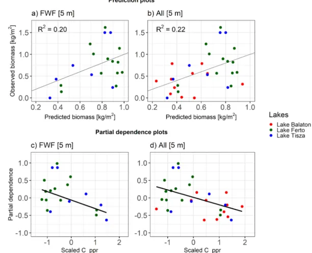
For the biomass estimation, the best R2 was achieved using the ALS points within a 5 m radius around the field observation points (Table 2).
Only the pulse penetration ratio (C_ppr) was required for both models (FWF and FWF combined with DR). The explained variance was slightly lower when using only the FWF ALS data (R2 =0.20) compared to using the combined ALS datasets (R2 =0.22).
The 5 m radius also produced the best results for the LAI (Table 2).
However, the explained variance was very low (R2 <0.3). The model at Lake Balaton included the 99th percentile of height (H_p99) and the standard deviation of amplitude (A_std) as predictor variables, whereas the models at Lake Ferto and Lake Tisza (both leaf-off and leaf-on ALS ˝ datasets) only included the pulse penetration ratio (C_ppr). The explained variance was low at Lake Balaton (R2 =0.29) and at Lake Tisza (R2 =0.26 for leaf-off and R2 =0.30 for leaf-on ALS data), and very low at Lake Fert˝o (R2 =0.08).
3.2. Effects of different data characteristics
3.2.1. Matching field samples with airborne laser scanning data
Sample size was substantially reduced when a search radius of 0.5 m Table 1
Derived LiDAR metrics for estimating vegetation structure in wetlands. Metrics capture radiometric and vegetation structural information (openness, height and vertical variability) at 0.5 m, 2.5 m and 5 m radius around the in-situ field observation points. z =normalized height value of the Airborne Laser Scanning (ALS) point.
Metric class Name of LiDAR metric Metric
abbreviation Description Reference
Radiometric
information Standard deviation of
amplitude A_std Standard deviation of signal strength within the search radius (Moeslund et al., 2019) Sum amplitude ratio A_cover Ratio of sum of the intensity of vegetation points to the sum of
intensity of points within the search radius (Luo et al., 2015) Vegetation
openness Pulse penetration ratio C_ppr Ratio of the number of ground points to the total number of points within the search radius
Vegetation height 99th percentile of z H_99p 99th percentile of z within the search radius (Hopkinson et al., 2005; Luo et al., 2017; Nie et al., 2018)
Mean z H_mean Mean of z within the search radius
Median of z H_median Median of z within the search radius Vertical variability Standard deviation of z V_std Standard deviation of z within the search radius
Variance of z V_var Variance of z within the search radius
was applied to ALS data with a low point density (4 pt/m2). This was because no ALS data points were available within a 0.5 m search radius around these field observation points. The reduction in sample size was largest for the DR ALS data (63%) and substantially lower for the low point density FWF ALS data (31%). For the high point density (18 pt/m2) FWF ALS data, all samples could be used. With a 5 m search radius, the retrieved number of ALS points was sufficient for calculating LiDAR metrics and all field observation points could be used for the modelling.
3.2.2. Effects of the characteristics of airborne laser scanning data Field-measured vegetation height was better explained by the FWF ALS data alone (Fig. 2a) then by a combination of FWF and DR ALS data (Fig. 2b). Nevertheless, in both cases there was a strong relationship between the ALS-derived vegetation height (H_p99) and the field- measured height (Fig. 2c,d). Field-measured biomass was similarly explained by the FWF and the combined FWF and DR data, but with a low R2 (Fig. 3a,b). The relationship between field-measured biomass and the most important LiDAR variable (pulse penetration ratio, C_ppr) was negative (Fig. 3c,d), predicting less vegetation biomass in more open vegetation. Field-measured LAI was generally best explained by a combination of LiDAR metrics (Table 2), with a similar explained vari- ance across lakes, recording types, point densities and seasons (Fig. 4a,c, d), except for FWF data at lake Ferto (Fig. 4c). The strongest LiDAR ˝ predictor variable of the LAI was either the 99th percentile of vegetation height (H_99p) or the pulse penetration ratio (C_ppr) (Fig. 4e–h).
The radius for extracting LiDAR metrics around the field observation points influenced the explained variance of the models (Table 2).
Explained variance of field-measured vegetation height was highest with LiDAR metrics calculated at a 0.5 m radius (R2 =0.84) and was strongly reduced with a 5 m radius (R2 =0.28). In contrast, the best models for field-measured biomass were achieved with LiDAR metrics calculated at a 5 m radius around the field observation points (Table 2).
Similarly, the explained variance of the LAI models tended to be best with a 5 m radius (Table 2).
The temporal offset and seasonality between the field and ALS data did not show an effect on the estimation of vegetation height and biomass because data points from different lakes tended to be spread equally across the prediction plots (Fig. 2a,b and Fig. 3a,b). The results of the LAI estimation at Lake Fert˝o (Fig. 4b) suggested that the temporal offset between the field measurements and the ALS data acquisition (5–6 years) might have masked a relationship between field data and LiDAR metrics. Seasonality of ALS data acquisition didn’t seem to have a strong effect because the FWF-based estimation of the LAI at Lake Tisza was equally well explained in March and June (Fig. 4c–d).
4. Discussion
Our study quantifies the extent to which ecological field measure- ments of vegetation height, biomass and LAI in wetlands can be related to 3D vegetation metrics derived from LiDAR. Using ALS data from three Hungarian lakes, we show that field-measured vegetation height can be effectively estimated using the 99th percentile of z-values from ALS data. This holds true across the different lakes at which ALS datasets have been obtained with different characteristics (FWF and DR recording types, varying point densities). In contrast, the estimation of field-measured biomass and LAI with LiDAR metrics proved to be poor and sensitive to differences in ALS characteristics as well as to discrep- ancies in spatial resolution, temporal offset and seasonality between ALS data acquisition and field sampling. Our results thereby provide important insights for the development of LiDAR-based ecological in- dicators of ecosystem structure in wetlands or other vegetation that shows similarity in physical structure to wetland vegetation.
Table 2
Results of multivariate regression models to explain field-based measurements of vegetation height, biomass and Leaf Area Index (LAI). Separate models are fitted for different airborne laser scanning (ALS) datasets (FWF, All) and three different spatial resolutions (0.5, 2.5 and 5 m radius around field observation points). Empty rows indicate that a model could not be fitted due to the low sample size. For abbreviations of LiDAR metrics see Table 1. p-value is *** if p <0.01, ** if p <0.05, * if p <0.1, ns =not significant. Models with the explained variance (R2) are highlighted in bold. R2 =explained variance, Adj. R2 =Adjusted explained variance, RSE =Residual Standard Error, p =statistical significance of F-statistic.
ALS data Radius Fitted model equation n R2 Adj. R2 RSE p
Vegetation height
Input LiDAR metrics (H_p99, C_ppr, A_std)
FWF 0.5 0.859 H_p99 +3.057 15 0.835 0.822 0.325 ***
FWF 2.5 0.661 H_p99 +0.395 C_ppr +3.145 19 0.435 0.365 0.603 **
FWF 5 0.490 H_p99 +3.102 20 0.325 0.288 0.626 ***
All 0.5 0.983 H_p99 +0.306 C_ppr − 0.450 A_std +3.345 19 0.671 0.605 0.474 ***
All 2.5 0.565 H_p99 +3.019 29 0.304 0.278 0.812 ***
All 5 0.631 H_p99 − 0.289 A_std +3.004 31 0.281 0.230 0.812 ***
Biomass
Input LiDAR metrics (H_p99, C_ppr, A_std)
FWF 0.5 –
FWF 2.5 −0.192 C_ppr +0.724 19 0.131 0.08 0.453 ns
FWF 5 −0.243 C_ppr +0.684 20 0.202 0.158 0.434 **
All 0.5 –
All 2.5 −0.201 C_ppr +0.654 29 0.194 0.164 0.417 **
All 5 −0.212 C_ppr +0.632 31 0.219 0.192 0.402 ***
LAI Input LiDAR metrics (H_p99, C_ppr, A_std)
Lake Balaton (Apr.) 0.5 0.358 C_ppr +3.668 34 0.060 0.03 1.414 ns
Lake Balaton (Apr.) 2.5 6.364 H_p99 − 0.836 A_std +4.931 56 0.289 0.263 1.423 ***
Lake Balaton (Apr.) 5 4.993 H_99p − 0.850 A_std +4.539 57 0.290 0.263 1.393 ***
Lake Ferto (Dec.) 0.5 –
Lake Ferto (Dec.) 2.5 −5.143 H_99p +0.267 A_std +2.717 54 0.085 0.05 1.153 ns
Lake Ferto (Dec.) 5 0.4 C_ppr +3.893 55 0.075 0.057 1.137 **
Lake Tisza (March) 0.5 –
Lake Tisza (March) 2.5 −0.565 C_ppr +3.587 31 0.211 0.183 0.942 ***
Lake Tisza (March) 5 −0.668 C_ppr +3.589 32 0.258 0.233 0.939 ***
Lake Tisza (Jun.) 0.5 −0.483 C_ppr +3.257 35 0.154 0.128 1.007 **
Lake Tisza (Jun.) 2.5 −0.466 C_ppr +3.074 38 0.203 0.181 0.986 ***
Lake Tisza (Jun.) 5 −0.585 C_ppr +2.933 39 0.296 0.277 0.954 ***
4.1. Estimating wetland vegetation structure from airborne laser scanning Our results for vegetation height are promising and in agreement with other studies that show that ALS can precisely measure the canopy height of emergent macrophytes in wetlands. Reported R2 values in previous wetland studies range from 0.4 to 0.85 (Luo et al., 2015; Nie et al., 2018; Corti Meneses et al., 2017) and are comparable with our results (R2 =0.84 and 0.67, respectively). However, a range of different LiDAR metrics have been used to estimate vegetation height in in wet- lands that are dominated by reed (Phragmites australis). Luo et al. (2015) reported that the standard deviation of height is the most important predictor variable in in a wetland National Park in China, whereas Nie et al. (2018), Corti Meneses et al. (2017) and Onojeghuo et al. (2010) used the maximum height of reedbeds at a single lake in China, Germany and England, respectively. We found that both the variance of z and the 99th percentile of z gave promising results for estimating vegetation height across different lakes, as both are highly correlated (r =0.91, see Fig. S2). This suggests that the variance of z and the 99th percentile of z are appropriate LiDAR metrics that can serve as ecological indicators for vegetation height across wetlands.
The estimation of vegetation biomass with LiDAR metrics only ach- ieved a low explained variance in our study (R2 =0.20–0.22). A study by Luo et al. (2017) in a reed (Phragmites australis) dominated wetland in China achieved an R2 =0.56 using only DR ALS data with simulta- neously measured field data and a larger sample size (n =75) than in our study (n =31). Another study (Riegel et al., 2013) reported R2-values comparable to ours (adj. R2 =0.18). Both studies (Riegel et al., 2013;
Luo et al., 2015) estimated field-measured vegetation biomass with height-related LiDAR metrics (99th percentile of z and the mean of z). In contrast, in our study the most relevant metric for estimating biomass was the pulse penetration ratio (C_ppr), a measure of vegetation open- ness. This difference could be explained by the use of FWF ALS data in our study, which can better capture ground points under the reed can- opies, compared to DR ALS data used in previous studies (Riegel et al., 2013; Luo et al., 2015). This could indicate that different LiDAR metrics (99th percentile of z and pulse penetration ratio) may be needed to derive ecological indicators for estimating vegetation biomass from ALS, depending on which ALS recording type is used (DR or FWF).
The LAI could not be well estimated in our study (R2 =0.08–0.30). In contrast, one study (Luo et al., 2015) showed that the LAI could be well estimated with LiDAR metrics (R2 = 0.79) at one reed-dominated wetland site in China. This difference could be explained by the sam- pling method of the LAI field measurements. Our study used photo- graphs from a zenith facing handheld digital camera. This can result in distortions which cannot be fully corrected during data pre-processing.
In contrast, Luo et al. (2015) used hemispherical photographs of a LAI- 2200 Plant Canopy Analyzer device with a fisheye optical sensor which can give more precise distortion free images for calculating LAI. Luo et al. (2015) further found that the use of the 99th percentile of z per- formed better than the pulse penetration ratio. Our study supports this finding in the case of DR ALS data where the AIC model selection excluded the pulse penetration ratio (C_ppr) from the LAI estimation.
For the development of ALS-based ecological indicators that quantify leaf area or other aspects of vegetation cover in wetlands, future studies Fig. 2. Visualization of the vegetation height model for full waveform data (FWF) and for FWF and discrete return data combined (All). (a,b) Prediction plots indicate the relationship between observed and predicted vegetation height based on the most parsimonious model (see Table 2). (c,d) Partial dependence plots show the relationship between field-measured vegetation height (y-axis) and LiDAR-derived vegetation height (Scaled H_p99). Colors of dots correspond to each lake (red =Lake Balaton, green =Lake Fert˝o and blue =Lake Tisza). (For interpretation of the references to colour in this figure legend, the reader is referred to the web version of this article.)
should further test to what extent the 99th percentile of z, the pulse penetration ratio, or other LiDAR metrics are robust and consistent with field-based measurements of LAI.
4.2. Effects of different data characteristics 4.2.1. Sampling of field data
Our vegetation height measures are methodologically similar to other studies (Luo et al., 2015; Nie et al., 2018; Corti Meneses et al, 2017; Onojeghuo et al., 2010). However, our field measurements of biomass and LAI differ from other studies. Luo et al. (2017) estimated vegetation biomass using an allometric equation with vegetation height.
This method allowed a fast data collection, since after establishing the allometric equation between the dry weight and the reed height, only the height needed to be measured in the field. In contrast, we directly measured biomass through harvesting above-ground vegetation parts in the field. This is a more time-intensive data collection method and resulted in a lower sample size compared to Luo et al. (2017). The LAI was measured by Luo et al., (2017) using a LAI-2200 Plant Canopy Analyzer device, which could result in more accurate measurements compare to our method (using a zenith facing handheld digital camera).
However, our LAI measurements are rapid and cost-effective and could thus be easily and widely applied in the field. Future studies should directly compare which estimation methods provide the most optimal field collection technique for measuring biomass and LAI within wetlands.
4.2.2. Effects of characteristics of airborne laser scanning data
We analyzed the effect of ALS data characteristics for quantifying vegetation structure within wetlands. Previous studies have shown that DR ALS data with low point densities have difficulties to capture ground points under a dense reed canopy (Luo et al., 2015; Nie et al., 2018;
Onojeghuo et al., 2010; Hopkinson et al., 2004). This is important because the accuracy of estimating vegetation height is influenced by whether the ALS sensor was able to detect ground points under the canopy. Our results suggest that FWF ALS data capture ground points sufficiently, even under leaf-on conditions, whereas DR ALS data do not.
For instance, visual inspection of ALS point clouds from crossplots at the three lakes showed that vegetation points are misclassified in DR data as ground points (Fig. 5a) whereas FWF ALS data correctly classify ground points under the reed canopy (Fig. 5b–d). The FWF ALS data save the whole waveform and the post-processing is thus able to detect subse- quent returns even with low intensity (Mallet and Bretar, 2009). The improved detection of ground points can increase the accuracy of the pulse penetration ratio, which is based on the ratio of ground points to the total number of points (Table 1). This can explain its importance as predictor variable for estimating biomass and LAI. Higher point den- sities (Lake Tisza) did not substantially improve the explained variance of the models in our study, which indicates that low point density FWF ALS data are already able to efficiently capture vegetation structural parameters across wetlands. Such FWF data are increasingly becoming available through national-scale scanning campaigns (Moeslund et al., 2019).
Fig. 3. Visualization of the biomass model for full waveform data (FWF) and for FWF and discrete return data combined (All). (a,b) Prediction plots indicate the relationship between observed and predicted biomass based on the most parsimonious model (see Table 2). (c,d) Partial dependence plots show the relationship between field-measured biomass (y-axis) and the LiDAR-derived biomass (Scaled C_ppr). Colors of dots correspond to each lake (red =Lake Balaton, green =Lake Ferto and blue ˝ =Lake Tisza). (For interpretation of the references to colour in this figure legend, the reader is referred to the web version of this article.)
4.2.3. Discrepancies between field and airborne laser scanning data Discrepancies between field and ALS data collection could be a main reason for the relatively low explained variance in estimating field- measured biomass and LAI from LiDAR metrics. In particular, discrep- ancies in the spatial resolution, the temporal offset between field and ALS data acquisition, and the seasonal dynamics of vegetation growth in wetlands may have an influence on how well LiDAR metrics can explain field measurements of vegetation structure. Regarding spatial resolu- tion, our results suggest that both biomass and LAI can be best explained from ALS data if LiDAR metrics are calculated with a radius that en- compasses an area larger than the plot size measured in the field. Similar results were obtained by Luo et al. (2017) who found the optimal sample radius for calculating LiDAR metrics for biomass to be 1.5 m larger than the 1 m ×1 m plot size for measuring the field data. The effect of the time difference between LIDAR and field data collection is closely con- nected to changes of wetland area and structure at the scale of several years. The structure of reed vegetation is expected to be relatively constant as it depends mainly on the presence of various ecotypes (T´oth and Szab´o 2012), but the location of the reed-water boundary can change up to several meters during a year (Zlinszky, 2013) For instance, the reed fronts at Lake Balaton are receding with reed die-back (Toth, ´ 2016), which could affect the relationship between field-measured vegetation structure and our calculated LiDAR metrics. At Lake Fert˝o, reed encroachment into open water is ongoing, which means that the temporal offset between ALS flights and fieldwork could result in field plots being surveyed in places where no vegetation was present during the flight campaign. The Lake Fert˝o dataset also had the largest time difference between the ALS and the field data (5–6 years). At Lake Tisza, most vegetation-water transition zones are determined by abrupt changes in water depth, e.g. due to flooded river arms. The water fronts are thus relatively stable and might be less affected by the time offset between the ALS and field data. These results overall suggest that the (near-) simultaneous measurement of field data with the ALS flight campaign is preferable if the aim of the study is to estimate 3D vege- tation structural parameters from LiDAR. Regarding the seasonal timing
of ALS data acquisition, previous studies show that ALS datasets ac- quired in spring and summer can perform similarly well when explain- ing wetland vegetation structure (Luo et al., 2015, 2017; Nie et al., 2018). However, ALS data collected in winter months have been re- ported to be limited in capturing the full variability of vegetation structure in reedbeds (Onojeghuo et al., 2010). This aligns with our findings at Lake Fert˝o where field measurements of biomass and LAI obtained in August were not well explained by ALS data collected in December.
5. Conclusions
ALS has great potential to measure various aspects of 3D vegetation structure in a spatially contiguous way and across broad spatial extents.
However, appropriate metrics and their relationships with field mea- surements of vegetation structure in wetlands remain little explored. We compared a set of field measurements of 3D vegetation structure (height, biomass and LAI) from three Hungarian lakes with LiDAR metrics derived from ALS point clouds that had varying data characteristics (DR or FWF recording type, different point densities, acquisition in different seasons) and found that vegetation height can be robustly estimated independent of the ALS data qualities. Hence, the LiDAR metric 99th percentiles of z can be used as a robust ecological indicator of vegetation height in wetlands and other vegetation with similar physical structure.
However, field measurements of biomass and LAI were only weakly explained by LiDAR metrics and were sensitive to ALS data character- istics (recording type, seasonality), the spatial resolution of LiDAR metric calculation, and the temporal offset between field measurements and ALS data acquisition. This indicates that the selection of ecological indicators for estimating biomass and LAI from ALS needs to be further tested. We further suggest that future studies could test the relationship between field measurements and LiDAR metrics in other vegetation with similar physical structure, for instance in agricultural crops (e.g. maize and wheat) or wetland vegetation in saline waters (e.g. > 1 m tall halophyte vegetation). For the future development of vegetation Fig. 4.Visualization of the Leaf Area Index (LAI) models separated by lake (colors) and the recording type of the airborne laser scanner (FWF =full waveform data, DR =discrete return data). The month of laser scanner recording is given in square brackets. The prediction plots (a,b,c,d) indicate the relationship between observed and predicted LAI based on the most parsimonious models (see Table 2). The partial dependence plots (e,f,g,h) show the relationship between field-measured LAI (y- axis) and the most important LiDAR predictor variable (Scaled C_ppr).
structural indicators from LiDAR in wetlands, we specifically recom- mend (i) to standardize and harmonize field collection protocols for measuring aspects of 3D vegetation structure which can be aligned with ALS data, (ii) to sample vegetation structure in several small sub-plots within larger (e.g. 10 m × 10 m) plots to enhance the alignment of field measurements with LiDAR metrics derived from varying point densities and ALS recording types, and (iii) to promote the FWF recording of ALS data among data suppliers for overcoming difficulties of capturing ground points in wetlands. Moreover, a close cooperation between ecologists and remote sensing scientists will be crucial for achieving this. Our results provide an important step towards the operational use of LiDAR for estimating wetland vegetation structure and for deriving indicators to monitor biodiversity and ecosystem change from ALS data.
6. Formatting funding resources
This work is part of the project “eScience infrastructure for Ecolog- ical applications of LiDAR point clouds” (eEcoLiDAR) (Kissling et al., 2017), funded by the Netherlands eScience Center (https://www.escie ncecenter.nl), grant number ASDI.2016.014. The work of AZ in this study was funded by the Hungarian National Research, Development and Innovation Office with grant OTKA PD 115833. We further acknowledge the ALS data collection at Lake Tisza within the Change- habitats2 project, at Lake Fert˝o within Genesee project and with the cooperation of Vienna University of Technology and the National Park Neusiedlersee.
CRediT authorship contribution statement
Zsofia Koma: ´ Conceptualization, Methodology, Formal analysis, Investigation, Visualization, Writing - original draft, Writing - review &
Fig. 5. Visualization of point clouds derived from different Airborne Laser Scanning (ALS) datasets for three Hungarian lakes. (a) Lake Balaton (discrete return ALS data with 4 pt/m2), (b) Lake Fert˝o (FWF ALS data with 4 pt/m2), and (c-d) Lake Tisza (FWF ALS data with 21 pt/m2 in March and 18 pt/m2 in June). The left side shows the point clouds extracted within a 25 m radius around each field observation point (indicated with a red triangle) and visualized according to the z-value (blue indicates low vegetation height and red high vegetation height). On the right, 25 m long crossplots in West-East direction with 2 m width are shown (green:
non-ground points, pink: ground points). DR =discrete return data, FWF =full waveform data, pt/m2 =points per square meter, W =west, E =east. (For interpretation of the references to colour in this figure legend, the reader is referred to the web version of this article.)
editing. Andr´as Zlinszky: Conceptualization, Investigation, Data cura- tion, Funding acquisition, Writing - review & editing. L´aszlo Bek´ o: Data ˝ curation, Formal analysis. P´eter Burai: Data curation. Arie C. Seij- monsbergen: Conceptualization, Supervision, Writing - review & edit- ing. W. Daniel Kissling: Conceptualization, Methodology, Supervision, Funding acquisition, Writing - review & editing.
Declaration of Competing Interest
The authors declare that they have no known competing financial interests or personal relationships that could have appeared to influence the work reported in this paper.
Appendix A. Supplementary data
Supplementary data to this article can be found online at https://doi.
org/10.1016/j.ecolind.2021.107752.
References
Bakx, T.R.M., Koma, Z., Seijmonsbergen, A.C., Kissling, W.D., 2019. Use and categorization of Light Detection and Ranging vegetation metrics in avian diversity and species distribution research. Divers. Distrib. 25 (7), 1045–1059. https://doi.
org/10.1111/ddi.12915.
Cao, L., Coops, N.C., Hermosilla, T., Innes, J., Dai, J., She, G., 2014. Using small-footprint discrete and full-waveform airborne LiDAR metrics to estimate total biomass and biomass components in subtropical forests. Remote Sens. 6, 7110–7135. https://doi.
org/10.3390/rs6087110.
Chasmer, L., Hopkinson, C., Montgomery, J., Petrone, R., 2016. A physically based terrain morphology and vegetation structural classification for wetlands of the Boreal Plains, Alberta, Canada. Can. J. Remote Sens. 42 (5), 521–540. https://doi.
org/10.1080/07038992.2016.1196583.
Corti Meneses, N., Baier, S., Geist, J., Schneider, T., 2017. Evaluation of Green-LiDAR Data for Mapping Extent, Density and Height of Aquatic Reed Beds at Lake Chiemsee, Bavaria—Germany. Remote Sens. 9, 1308. https://doi.org/10.3390/
rs9121308.
Davies, A.B., Asner, G.P., 2014. Advances in animal ecology from 3D-LiDAR ecosystem mapping. Trends Ecol. Evol. 29 (12), 681–691. https://doi.org/10.1016/j.
tree.2014.10.005.
Fliervoet, L.M., Werger, M.J.A., 1984. Canopy structure and microclimate of two wet grassland communities. New Phytol. 96 (1), 115–130. https://doi.org/10.1111/
j.1469-8137.1984.tb03548.x.
Hall, F.G., Bergen, K., Blair, J.B., Dubayah, R., Houghton, R., Hurtt, G., Kellndorfer, J., Lefsky, M., Ranson, J., Saatchi, S., Shugart, H.H., Wickland, D., 2011. Characterizing 3D vegetation structure from space: Mission requirements. Remote Sens. Environ.
115 (11), 2753–2775. https://doi.org/10.1016/j.rse.2011.01.024.
Hladik, C., Alber, M., 2012. Accuracy assessment and correction of a LIDAR-derived salt marsh digital elevation model. Remote Sens. Environ. 121, 224–235. https://doi.
org/10.1016/j.rse.2012.01.018.
H¨ofle, B., Pfeifer, N., 2007. Correction of laser scanning intensity data: data and model- driven approaches. ISPRS J. Photogramm. Remote Sens. 62 (6), 415–433. https://
doi.org/10.1016/j.isprsjprs.2007.05.008.
Hopkinson, C., Chasmer, L., Lim, K., Treitz, P., Creed, I., 2006. Towards a universal lidar canopy height indicator. Can. J. Remote Sens. 32 (2), 139–152. https://doi.org/
10.5589/m06-006.
Hopkinson, C., Chasmer, L.E., Sass, G., Creed, I.F., Sitar, M., Kalbfleisch, W., Treitz, P., 2005. Vegetation class dependent errors in lidar ground elevation and canopy height estimates in a boreal wetland environment. Can. J. Remote Sens. 31 (2), 191–206.
https://doi.org/10.5589/m05-007.
Hopkinson, C., Lim, K., Chasmer, L.E., Treitz, P., Creed, I.F., Gynan, C., 2004. Wetland grass to plantation forest-estimating vegetation height from the standard deviation of lidar frequency distributions. Int. Arch. Photogramm. Remote Sens. Spat. Inf. Sci.
36 (8), 288–294.
Hyypp¨a, J., Hyypp¨a, H., Leckie, D., Gougeon, F., Yu, X., Maltamo, M., 2008. Review of methods of small-footprint airborne laser scanning for extracting forest inventory data in boreal forests. Int. J. Remote Sens. 29 (5), 1339–1366. https://doi.org/
10.1080/01431160701736489.
Jonckheere, I., Fleck, S., Nackaerts, K., Muys, B., Coppin, P., Weiss, M., Baret, F., 2004.
Review of methods for in situ leaf area index determination: Part I. Theories, sensors and hemispherical photography. Agric. For. Meteorol. 121 (1-2), 19–35. https://doi.
org/10.1016/j.agrformet.2003.08.027.
Kissling, W.D., Seijmonsbergen, A., Foppen, R., Bouten, W., 2017. eEcoLiDAR, eScience infrastructure for ecological applications of LiDAR point clouds: reconstructing the 3D ecosystem structure for animals at regional to continental scales. Res. Ideas Outcomes 3, e14939. https://doi.org/10.3897/rio.3.e14939.
Koma, Z., Rutzinger, M., Bremer, M., 2018. Automated segmentation of leaves from deciduous trees in terrestrial laser scanning point clouds. IEEE Geosci. Remote Sensing Lett. 15 (9), 1456–1460. https://doi.org/10.1109/LGRS.2018.2841429.
Koma, Z., Seijmonsbergen, A.C., Kissling, W.D., 2021. Classifying wetland-related land cover types and habitats using fine-scale lidar metrics derived from country-wide
Airborne Laser Scanning. Remote Sens. Ecol. Conserv. 7 (1), 80–96. https://doi.org/
10.1002/rse2.170.
Korpela, I., Hovi, A., Morsdorf, F., 2012. Understory trees in airborne LiDAR data — selective mapping due to transmission losses and echo-triggering mechanisms.
Remote Sens. Environ. 119, 92–104. https://doi.org/10.1016/j.rse.2011.12.011.
Lefsky, M.A., Cohen, W.B., Parker, G.G., Harding, D.J., 2002. Lidar Remote Sensing for Ecosystem Studies: Lidar, an emerging remote sensing technology that directly measures the three-dimensional distribution of plant canopies, can accurately estimate vegetation structural attributes and should be of particular interest to forest, landscape, and global ecologists. BioScience 52, 19–30. https://doi.org/
10.1641/0006-3568(2002)052[0019:LRSFES]2.0.CO;2.
Liu, J., Pattey, E., 2010. Retrieval of leaf area index from top-of-canopy digital photography over agricultural crops. Agric. For. Meteorol. 150 (11), 1485–1490.
https://doi.org/10.1016/j.agrformet.2010.08.002.
Luo, S., Wang, C., Pan, F., Xi, X., Li, G., Nie, S., Xia, S., 2015. Estimation of wetland vegetation height and leaf area index using airborne laser scanning data. Ecol. Indic.
48, 550–559. https://doi.org/10.1016/j.ecolind.2014.09.024.
Luo, S., Wang, C., Xi, X., Pan, F., Qian, M., Peng, D., Nie, S., Qin, H., Lin, Y., 2017.
Retrieving aboveground biomass of wetland Phragmites australis (common reed) using a combination of airborne discrete-return LiDAR and hyperspectral data. Int. J.
Appl. Earth Obs. Geoinformation 58, 107–117. https://doi.org/10.1016/j.
jag.2017.01.016.
Mallet, C., Bretar, F., 2009. Full-waveform topographic lidar: State-of-the-art. ISPRS J.
Photogramm. Remote Sens. 64 (1), 1–16. https://doi.org/10.1016/j.
isprsjprs.2008.09.007.
Maltamo, M., Næsset, E., Vauhkonen, J. (Eds.), 2014. Forestry Applications of Airborne Laser Scanning, Managing Forest Ecosystems. Springer Netherlands, Dordrecht.
https://doi.org/10.1007/978-94-017-8663-8.
Meijer, C., Grootes, M.W., Koma, Z., Dzigan, Y., Gonçalves, R., Andela, B., van den Oord, G., Ranguelova, E., Renaud, N., Kissling, W.D., 2020. Laserchicken—A tool for distributed feature calculation from massive LiDAR point cloud datasets. SoftwareX 12, 100626. https://doi.org/10.1016/j.softx.2020.100626.
Millard, K., Richardson, M., 2013. Wetland mapping with LiDAR derivatives, SAR polarimetric decompositions, and LiDAR–SAR fusion using a random forest classifier.
Can. J. Remote Sens. 39 (4), 290–307. https://doi.org/10.5589/m13-038.
Mitchley, J., Willems, J.H., 1995. Vertical canopy structure of Dutch chalk grasslands in relation to their management. Vegetatio 117 (1), 17–27. https://doi.org/10.1007/
BF00033256.
Moeslund, J.E., Zlinszky, A., Ejrnæs, R., Brunbjerg, A.K., Bøcher, P.K., Svenning, J.-C., Normand, S., 2019. Light detection and ranging explains diversity of plants, fungi, lichens, and bryophytes across multiple habitats and large geographic extent. Ecol.
Appl. 29 (5) https://doi.org/10.1002/eap.1907.
Nayegandhi, A., Brock, J.C., Wright, C.W., O’Connell, M.J., 2006. Evaluating A Small Footprint, Waveform-resolving Lidar Over Coastal Vegetation Communities.
Photogramm. Eng. Remote Sens. 72, 1407–1417. https://doi.org/10.14358/
PERS.72.12.1407.
Nie, S., Wang, C., Xi, X., Luo, S., Li, S., Tian, J., 2018. Estimating the height of wetland vegetation using airborne discrete-return LiDAR data. Optik 154, 267–274. https://
doi.org/10.1016/j.ijleo.2017.10.016.
Onojeghuo, A.O., Blackburn, G.A., 2013. Characterising reedbeds using LiDAR data:
potential and limitations. IEEE J. Sel. Top. Appl. Earth Obs. Remote Sens. 6 (2), 935–941. https://doi.org/10.1109/JSTARS.2012.2212235.
Onojeghuo, A.O., Blackburn, G.A., Latif, Z.A., Characterising Reedbed habitat quality using Leaf-off LiDAR Data, in: 2010 6th International Colloquium on Signal Processing Its Applications. Presented at the 2010 6th International Colloquium on Signal Processing its Applications, 2010, pp. 1–5. doi: 10.1109/
CSPA.2010.5545322.
Pereira, H.M., Ferrier, S., Walters, M., Geller, G.N., Jongman, R.H.G., Scholes, R.J., Bruford, M.W., Brummitt, N., Butchart, S.H.M., Cardoso, A.C., Coops, N.C., Dulloo, E., Faith, D.P., Freyhof, J., Gregory, R.D., Heip, C., H¨oft, R., Hurtt, G., Jetz, W., Karp, D.S., McGeoch, M.A., Obura, D., Onoda, Y., Pettorelli, N., Reyers, B., Sayre, R., Scharlemann, J.P.W., Stuart, S.N., Turak, E., Walpole, M., Wegmann, M., 2013. Essential biodiversity variables. Science 339 (6117), 277–278. https://doi.
org/10.1126/science:1229931.
Riegel, J.B., Bernhardt, E., Swenson, J., 2013. Estimating above-ground carbon biomass in a newly restored coastal plain wetland using remote sensing. PLoS ONE 8 (6), e68251. https://doi.org/10.1371/journal.pone.0068251.
Roussel, J.-R., Auty, D., Coops, N.C., Tompalski, P., Goodbody, T.R.H., Meador, A.S., Bourdon, J.-F., de Boissieu, F., Achim, A., 2020. lidR: an R package for analysis of Airborne Laser Scanning (ALS) data. Remote Sens. Environ. 251, 112061. https://
doi.org/10.1016/j.rse.2020.112061.
Serbin, S.P., Townsend, P.A., 2020. Scaling functional traits from leaves to canopies. In:
Cavender-Bares, J., Gamon, J.A., Townsend, P.A. (Eds.), Remote Sensing of Plant Biodiversity. Springer International Publishing, Cham, pp. 43–82. https://doi.org/
10.1007/978-3-030-33157-3_3.
Shan, J., Toth, C.K., 2018. Topographic Laser Ranging and Scanning: Principles and Processing, Second ed. CRC Press, Boca Raton FL.
T´oth, V.R., 2016. Reed stands during different water level periods: physico-chemical properties of the sediment and growth of Phragmites australis of Lake Balaton.
Hydrobiologia 778 (1), 193–207. https://doi.org/10.1007/s10750-016-2684-z.
T´oth, V.R., Szab´o, K., 2012. Morphometric structural analysis of Phragmites australis stands in Lake Balaton. Ann. Limnol. - Int. J. Lim. 48 (2), 241–251. https://doi.org/
10.1051/limn/2012015.
Ussyshkin, V., Theriault, L., 2011. Airborne Lidar: advances in discrete return technology for 3D vegetation mapping. Remote Sens. 3, 416–434. https://doi.org/10.3390/
rs3030416.
Valbuena, R., O’Connor, B., Zellweger, F., Simonson, W., Vihervaara, P., Maltamo, M., Silva, C.A., Almeida, D.R.A., Danks, F., Morsdorf, F., Chirici, G., Lucas, R., Coomes, D.A., Coops, N.C., 2020. Standardizing ecosystem morphological traits from 3D information sources. Trends Ecol. Evol. 35 (8), 656–667. https://doi.org/
10.1016/j.tree.2020.03.006.
Zhang, K., Whitman, D., 2003. A progressive morphological filter for removing nonground measurements from airborne LIDAR data. IEEE Trans. Geosci. Remote Sens. 41, 872–882. https://doi.org/10.1109/TGRS.2003.810682.
Zlinszky, A., 2013. Mapping and conservation of the reed wetlands on Lake Balaton. PhD Thesis. E¨otv¨os Lor´and University, Budapest.
Zlinszky, A., Mücke, W., Lehner, H., Briese, C., Pfeifer, N., 2012. Categorizing wetland vegetation by airborne laser scanning on lake balaton and kis-balaton, Hungary.
Remote Sens. 4, 1617–1650. https://doi.org/10.3390/rs4061617.