L OCATING AND PARAMETER RETRIEVAL OF INDIVIDUAL TREES FROM TERRESTRIAL LASER SCANNER DATA

(1)

# 307

L OCATING AND PARAMETER RETRIEVAL OF INDIVIDUAL TREES FROM TERRESTRIAL LASER SCANNER DATA

Gábor Béla Brolly

The University of West Hungary (Sopron)

Roth Gyula Doctoral School of Forestry and Wildlife Management Sciences Course Forest Assets Management (E3)

Supervisor: associate professor Dr. Kornél Czimber Inst. of Geomatics and Civil Engineering

Dept. of Surveying and Remote Sensing

Sopron 2013

(2)

(3)

LOCATING AND PARAMETER RETRIEVAL OF INDIVIDUAL TREES FROM TERRESTRIAL LASER SCANNER DATA

Értekezés doktori (PhD) fokozat elnyerése érdekében Írta:

Brolly Gábor Béla

Készült a Nyugat-magyarországi Egyetem Roth Gyula Erdészeti és Vadgazdálkodási Tudományok Doktori Iskola Erdővagyon-gazdálkodás programja keretében Témavezető: Dr. Czimber Kornél egyetemi docens

Elfogadásra javasolom (igen / nem)

(aláírás) A jelölt a doktori szigorlaton …... % -ot ért el,

Sopron,…...

a Szigorlati Bizottság elnöke Az értekezést bírálóként elfogadásra javasolom (igen / nem)

Első bíráló (Dr. …... …...) igen /nem

(aláírás) Második bíráló (Dr. …... …...) igen /nem

(aláírás)

(Esetleg harmadik bíráló (Dr. …... …...) igen /nem

(aláírás) A jelölt az értekezés nyilvános vitáján…...% - ot ért el

Sopron,

………...

a Bírálóbizottság elnöke

A doktori (PhD) oklevél minősítése…...

………..

Az EDT elnöke

(4)

Abstract / Kivonat

The thesis introduces algorithms developed by the author allowing highly automated processing of terrestrial laser scanner data recorded in uneven-aged, temperate forests with multiple canopy layers and undergrowth. The extraction of tree positions is achieved in irregular as well as in regular data structures of two and three dimensions using a clustering technique and the concept of disconnected image objects. The two-dimensional methods deliver the parametric models of the stems’ cross-section, while the three-dimensional ones reveal the complete tree structure through a regular grid model. The models provide means for the estimation of essential tree metrics, such as stem diameter at breast height, tree height and horizontal crown projection area. The algorithms were validated with laser scans captured in stands of close-to-nature conditions. The algorithms provide a tool for tree locating and parameter retrieval even in the presence of low vegetation; furthermore, the mapping can be extended to the juvenile trees within the regeneration patches. The algorithms have potential in supporting forest inventories and in providing an objective data pool for scientific studies on forest dynamics.

Az értekezés olyan saját fejlesztésű eljárásokat mutat be, melyek többkorú, szintezett, aljnövényzettel rendelkező faállományokban is lehetővé teszik földi lézeres letapogatással felmért fák adatainak magas fokon automatizált feldolgozását. A faegyedek azonosítása síkbeli és térbeli, valamint szabályos és szabálytalan adatmodelleken történik az adatok particionálásával, valamint nem folytonos képi objektumokon végzett alakfelismeréssel. A síkbeli eljárások az azonosított faegyedek törzsének keresztmetszetének parametrikus leírását szolgáltatják, míg a térbeliek a fa szerkezetének térbeli rácsmodelljét (voxel modelleket). A modellek alapján a mellmagassági átmérő, a famagasság, és a koronavetületet mint a faegyedek legfontosabb mennyiségi állapotjellemzői határozhatók meg. Az eljárások tesztelése természetszerű állapotú faállományokban készült felmérések adatain történt. A javasolt eljárásokkal a fák térképezése aljnövényzet jelenlétében is hatékonyan elvégezhető, továbbá kiterjeszthető az újulati foltokban található egyedekre is. Az eljárások hatékonyan segíthetik az erdőleltározást, valamint objektív alapadatokat nyújthatnak az erdődinamikai vizsgálatokhoz.

(7)

1. Introduction

Tree maps depict the location of trees in a cartographic projection system and optionally other attributes at an individual level, resulting in a combination of spatial and biophysical features in a geographic information system. Tree models can be regarded as the extension of tree maps as they resemble the size and shape of the objects in addition to their positions, allowing direct estimation of structure-related tree metrics. Tree maps and tree models are increasingly used in fields of applications as diverse as forest inventory, forest monitoring, civil engineering, as well as the simulation of forest dynamics. However, the surveying of vegetation introduces many specific requirements, and thus data acquisition and processing is still challenging over forested areas.

Terrestrial laser scanning is an active remote sensing technology that provides coordinates of the surface of objects by laser range finding in a regular pattern with a high sampling density. It has the ability to acquire some millions of surface point coordinates with positional accuracy of a few millimetres within an area of 0.01–1 hectare per scanning positions in forested environment. Because of 3D data acquisition principle, the processing workflow can be automated to a high degree. Efficient data acquisition in combination with automatic processing offers a powerful solution for tree mapping and parameter retrieval. Automated processing protocols have the additional advantage of being objective and repeatable, which makes them promising for forest inventory and monitoring systems of regional scale. As the laser scans provide data on tree structure with high sampling density, structural parameters can be achieved that exceed the possibilities of the present dendrometric devices.

Consequently, the use of terrestrial laser scanner data has good prospects for describing complex forest structures, such as close-to-nature stands, and forest reserves. Nevertheless, commercially available software packages have been developed for extracting models of artificial objects within urbanized environments, but have limitations in processing the laser scanner data recorded in forested areas. In order to exploit the advantages of terrestrial laser scanning in tree mapping, specific algorithms need to be optimised for the detection and modelling of trees.

This thesis introduces algorithms developed by the author, which aim to automate tree locating and individual tree parameter retrieval from terrestrial laser scans. The algorithms are optimized for diverse structural characteristics, such as uneven-aged, multi-layered, mixed stands including regrowth patches. In addition to the survey of old-growth trees and the assessment of standard parameters (stem diameter and tree height), algorithms for detecting juvenile trees and for estimates of individual crown projection area are presented. The algorithms resulted in 2D parametric models of stem cross-sections and 3D grid models of the complete trees, from which the positions and biophysical attributes can be directly estimated.

The performance of the algorithms in terms of detection reliability and estimation accuracy was validated on test sites established in Hungarian forests with diverse stand structure.

(8)

2. Literature overview

2.1. Laser scanning

Laser scanning or LiDAR (Light Detection and Ranging) is an active remote sensing technology using laser range findings in regular pattern for data capture. Laser beam is characterized by high emission power, narrow beam width, well-defined frequency (monochromatic) and coherent radiation which allows for directional illumination and short pulse duration. As a result, the range finding systems have the ability of high accuracy and high measuring frequency. The wavelength used for the distance measurement is in the domain of visible light and near infrared electromagnetic radiation. The laser beam illuminates the surface of the target objects in an elliptical area called footprint. The distance between the instrument and the object can be calculated through the two-path runtime of the reflected signal. Measuring the polar and azimuthal direction of the emitted laser beam, the 3D coordinates of the reflection can be allocated in the sensor’s own coordinate system.

Laser scanners are data capture devices composed of two principal components: the range finding system and the beam deflection unit. In the course of the data acquisition, the scanner samples the target object with high frequency (10–1000 kHz) measurements that resulted in a high density and spatially explicit description of the object surfaces. Spectral parameters (e.g.

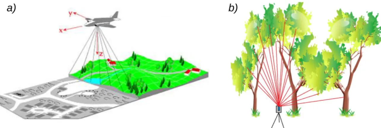
intensity, amplitude, beam width) can be recorded additionally that characterize the reflectance properties of the target object. The platform of the sensor can be a fixed tripod, motor vehicle, aircraft or satellite; upon which ground based or terrestrial (TLS), mobile, airborne (ALS) and spaceborne laser scanning systems are distinguished (Figure 2-1).

Laser scanning is subdivided further according to the ranging principle and the footprint size. The sensor alternatively records the round trip time of the pulse, the incident phase of a continuous wave, the full waveform of the reflected signal, or angles at widened laser illumination upon which pulse ranging, phase comparison, waveform analysis and triangulation-based ranging principles are distinguished (Pfeifer and Briese, 2007). In case of small footprint laser scanning, the footprint size is usually smaller than the surface of the target object. At large footprint laser scanning, the footprint radius is in the order of some ten meters so the laser beam illuminates multiple targets that cannot be separated. Spaceborne laser scanning is characterized by typically full waveform and large footprint technique, while airborne laser scanning utilizes small footprint and either pulse ranging or full waveform recording. Terrestrial laser scanners generally belong to the group of small footprint sampling instruments using pulse ranging or phase comparison principle, although some recent sensor digitize the full waveform as well. Scanners using the triangulation principle are ground- based. As they are restricted in ranging to a few metres, they are used principally indoor. The typical configurations of laser scanner systems regarding to the platform, ranging principle and footprint size are given in Table 2-1.

Table 2-1. Typical configurations of laser scanning systems.

Platform

Pulse ranging Phase shift Full-waveform Small Large

Spaceborne * *

Airborne * * *

Terrestrial * * *

Ranging principle Footprint

(9)

Figure 2-1. Examples on laser scanning from a) airborne and b) terrestrial platforms.(www.toposys.com, www.avf.forst.uni-goettingen.de)

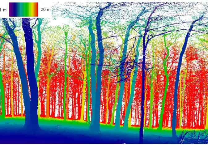
The primary output of laser scanning is referred to as point cloud (Figure 2-2) containing 3D coordinates and optionally descriptive data about the reflectance properties of the target surface. The point cloud is defined in the sensor’s coordinate system. If the point measurements are required to be located in a geodetic projection system or the spatial integration of data from different scans is needed, the transformation of the point cloud becomes necessary. The point cloud lacks any kind of spatial structure or explicit thematic information. The absence of the spatial structure means that the point cloud is stored as a sequential list without any explicit information on the neighbourhood relations. As a result, the number, the shape and size of the surveyed objects are unknown. In the absence of thematic information, the semantic meaning cannot be specified i.e. what the object is from which the laser beam was reflected. The point cloud is a kind of model that holds data on every surveyed object without regarding its relevance for the mapping purpose. One of the main goals in the data processing is to filter the members of the point cloud focusing on the thematic class of the targets to be mapped. The modelling of the target objects takes place following the classification procedure. The range of possible model types involves colour coded point clouds, triangulated meshes, grid models, composition of parametric surface patches, and 3D object models constructed of solid primitives. Due to the high sampling density, the models are generated ordinarily through the approximation of the point measurements. Beyond the surveying of topography, the accurate and spatially explicit models allows for revealing the structure of complex constructions and vegetated areas as well as their temporal changes (e.g. Wulder et al. (2007), Lovas et al., (2009)). Lovas et al.

(2012) provide comprehensive overview on laser scanning and its applications in Hungarian.

Figure 2-2. Point cloud from small footprint airborne laser scanning. (Source data: Sopron, Hungary, 2007.

Captured by GEOService Ltd. Figure compiled by the author.)

(10)

Terrestrial laser scanning is an active remote sensing technique operating from fixed ground based position and using laser range finding with high measuring frequency to obtain directly 3D coordinates (and optionally reflectance data) of high spatial density and high accuracy from object surfaces. The general processing of the point cloud data essentially covers the georeferencing of the point measurements, filtering data with regard to the objects to be mapped, and creation of spatially detailed models with high accuracy.

2.2. Terrestrial laser scanners

Terrestrial laser scanners composed of two main parts: the laser range finding system and the beam deflection unit. Concerning the measurement range, object scanners and surveying scanners can be differentiated. Only the latter meets the requirements of forest-mapping purposes allowing ranging in a distance of up to some hundred meters or even more.

The widely used surveying terrestrial laser scanners use either pulse ranging or phase comparison as a range finding principle. Pulse ranging systems calculate the distance by the time span between the emission and the detection of the laser signal assuming constant propagation of the laser light. At the phase comparison technique, the emitted laser signal is a continuous wave modulated on frequency. The distance of the reflection within the range of the modulated wavelength is determined through measuring the incident phase. Range measures exceeding the wavelength of modulation are ambiguous. Practically, the instruments utilize multiple modulation wavelengths for the extension of the effective range: The incident phase of the longer wavelengths is used to resolve the phase ambiguity of the shorter ones, which resulted in accurate distance even at long-range measurements. The distinct ranging principles resulted in differences in the effective range, precision, and scanning frequency.

Pulse ranging commonly provides longer effective ranging while the phase comparison technique delivers higher precision and higher measurement frequency. However, the performance of recent laser scanners using different ranging principles has been converging.

Waveform digitization has not become widespread in terrestrial laser scanners so far, although a few examples are already exists. Waveform digitizing systems record the complete backscattered waveform at constant time intervals during the acquisition. It has the advantage that additional descriptive data can be derived from the reconstructed signal (Wagner, 2005).

The temporal position of the target with respect to the transmitted pulse gives the absolute target range. The width of the echo provides information on the surface roughness or the direction of the target surface, while the amplitude of the echo is proportional to the target’s reflectance. When the laser beam contacts with multiple targets, each of them results a peak in the recorded signal (multiple echoes).

Frölich (2004) distinguishes three types of beam deflection units with respect to sensor’s field of view (Figure 2-3). Present classification of the instruments is limited to the typical constructions, although hybrid variants also exist.

1. Line scanners or profiling systems emit laser beams only in one direction and allocate them by a rotating mirror in the plane round about the axis. To produce a 3D point cloud, the sensor has to be moved along the direction of the axis so instruments of these types are rather applicable at mobile mapping, traffic security applications and vehicle control systems.

2. Camera view systems (frame scanners) are equipped with two oscillating or rotating mirrors, deflecting the laser light in horizontal and in vertical plane with a field of view about 60 degrees in both direction. The allocation of the laser beam in the vertical plane is called line scanning, while the horizontal one is called frame scanning.

(11)

of this type use similar technique for line scanning as the camera view systems, but the frame scanning is achieved by a slower rotation of the whole sensor body round about the polar instrument axis. The angle of view is full around in horizontal plane and 270–320 degree in vertical plane. Instruments having limited zenith angle enable the polar axis to be tilt in order to capture data from arbitrary part of the upper hemisphere. Figure 2-4 illustrates the main components of a (panoramic view) laser scanner system on the example of Riegl LMS Z420i.

Figure 2-3. Scanners’ field of view: (a) line scanner (b) frame scanner (c) panoramic scanner with limited upper zenith angle (d) panoramic scanner with full view over the upper hemisphere. (Illustrated by the author)

Terrestrial laser scanners optionally record spectral data characterizing the reflectivity of the target surface. The most common descriptive feature is the intensity of the reflected pulse.

State-of-art instruments digitize the full waveform of the emitted and reflected laser signal.

Following the waveform decomposition, multiple returns can be distinguished and the accuracy of the ranging can be enhanced by post-processing analysing of the signal waveform. In addition, the amplitude and echo width can be derived for each reflection.

Numerous scanners capture RGB data simultaneously with the ranging. Some earlier devices have mount points for external digital camera, while the newer ones contain built-in camera.

External cameras generally deliver images of higher quality, although they are more eccentric relative to the laser sensor. The range of the further optional extra supplies involves internal memory for on-board data recording, GNSS receiver, biaxial inclination sensor and compass for direct georeferencing, various standard interfaces (incl. WLAN, USB, Fire-wire, etc.), and colour touch screen.

Figure 2-4. The main components of laser scanner system on the example of Riegl LMS Z420i (www.riegl.com).

(12)

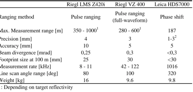
Table 2-2 introduces the technical parameters of three recent TLS devices depicted in Figure 2-5. The sample data for the evaluation of the algorithm described in this thesis were collected using an instrument Riegl LMS Z420i that stood for a state-of-art laser scanner around 2005. The VZ 400 belongs to the subsequent generation of pulse ranging Riegl scanners. The development of the past years can be noted on the example of these two instruments through the extension of full-waveform digitization capacity, increase of the measurement rate in the order of one magnitude, the reduction in weight by 40% and the integration of GNSS receiver as well as internal memory. The third instrument, the Leica HDS 7000 is an example to an up-to-date scanner using phase comparison ranging technique.

Its technical parameters reflect the main characteristic features of the phase comparison ranging principle: the higher scanning rate and the limited effective range. The precision is slightly better as it is at the pulse ranging instruments. All the instruments use eye-safe class laser so no additional equipment for protection is needed for the operation.

Figure 2-5. Examples on recent terrestrial laser scanners a) Riegl LMS-Z 420i (pulse ranging) b) Riegl VZ400 (pulse ranging with full waveform digitization) c) Leica HDS7000 (phase shift) (www.riegl.com, www.leica-

geosystems.com).

Table 2-2. Examples on the technical parameters of recent terrestrial laser scanners (www.riegl.com, www.leica-geosystems.com).

Riegl LMS Z420i Riegl VZ 400 Leica HDS7000

Ranging method Pulse ranging Pulse ranging

(full-waveform) Phase shift

Max. Measurement range [m] 350 - 1000¹ 280 - 600¹ 187

Precision [mm] 4 3 1-3²

Accuracy [mm] 10 5 5

Beam divergence [mrad] 0,25 0,3 <0,3

Footprint size at 100 m [mm] 25 30 <30

Measurement rate [kHz] 8 - 11 42 - 122 1016

Line scan angle range [deg] 80 100 320

Weight [kg] 16 9.6 9.8

1: Depending on target reflectivity

2: At 50 m distance, depending on target reflectivity

a) b) c)

(13)

should be paid for the reduction in the effective range by up to 50% resulting from the low reflectivity and rough surface of tree bark (www.riegl.com). Scanners with effective range of at least 50 meter are required for individual tree locating. Thin twigs and leaves may cause multiple echoes that result in invalid point measurements (ghost points) in the point cloud (Bienert et al, 2006). In addition, the reflections from trees beyond the ambiguity interval of the instruments using phase comparison ranging principle raise the proportion of measurement noise. Instruments with ranging accuracy in the order of 1 cm deemed appropriate for forestry applications, which is fulfilled by almost any of the recent scanners. A more crucial parameter is the scanning rate: Trees from afar of the sensor can be interpreted better as well as the tree tops can be located with higher accuracy in a dense point cloud data.

Furthermore, the higher scanning rate reduces the time of data collection that resulted in fewer ghost points at the tree crowns moved by the wind (Henning and Radtke, 2006a). Ducey et al.

(2013) found that the smaller footprint size leads to better penetration through the understory vegetation, although the larger footprint size is better suited for the identification of tree tops.

To provide complete sampling of the tree crown, instruments of those should be preferred that enable data capture from the entire upper hemisphere without changing the tilt angle of the polar axis. RGB data have the advantage at interpretation aiming at species classification.

Additionally, low weight, built-in power supply and compact design are necessary for the effective and convenient use over rural circumstances.

Full-waveform laser scanning holds great promise for forestry applications. Echo amplitude was found to be diagnostic feature in full-waveform airborne laser scans at the estimate of mixture rate of conifers and deciduous trees in leaf-less state (Brolly and Király, 2009b). It is expected that the spectral data of the terrestrial waveform recording systems can be similarly sufficient in distinguishing groups of tree species. Beside the amplitude, the echo width has potential in tree species classification through the quantification of bark roughness.

Multiple targets that are close to each other cause invalid (ghost) points because the echoes are superposed and their average range is returned. This issue may occur regardless to the type of laser ranging. Using full-waveform digitization, the echo shape indicates whether an echo originates from a single target or multiple targets, thus the number of ghost points can be suppressed. As low vegetation produce multiple echoes as well, this capability can also be efficient in their automatic filtering. Moreover, waveform digitization enables the detection of multiple echoes per pulse if the distance between the targets exceeds the minimum of multi- target resolution. With regard to forestry, multiple echo detection is prosperous for describing the fine structure of branching in the canopy. Studies on the benefit of full-waveform digitization in the field of forestry are required to verify these assumptions.

2.3. Transformation of the point cloud

The point cloud is defined by spherical coordinates (r,,) in the scanner’s own coordinate system, where r denotes the range,  and  describe the orientation of the directed laser beam in azimuthal and polar directions respectively (Figure 2-6). Although the raw observables deliver polar coordinates, most software packages provide rectangular coordinates (x,y,z) as output. The relationship between the raw observables and the rectangular coordinates can be expressed as follows (Reshetyuk, 2009):

(14)











































 sin

cos sin

cos cos r z y x

(2-1) Each point cloud is defined in the scanner’s own coordinate system, so transformations are needed to combine scans recorded from different positions and to locate the merged point cloud in a superior coordinate system (e.g. Hungarian Projection System EOV). The process of transforming each local coordinate system into a common coordinate system is generally referred to as relative orientation or specifically in case of terrestrial laser scans; registration.

The subsequent transformation of the combined point cloud into an earth-fixed coordinate system is achieved through the process of absolute orientation or georeferencing (Pfeifer and Briese, 2007).

z

y

x 



Figure 2-6. Raw observables in the sensor’s own coordinate system.

Both type of orientations realized as congruency transformation that preserves the distance and angle between any of the point pairs within the same scan. The number of parameters is six including a t(x,y,z)translation vector and



,,



rotation angles around each axis of the local sensor coordinate system. Let denote p_i(x_i,y_i,z_i) local coordinates of the i-th element in the point cloud, p^,_i the coordinates in the target reference system, Rthe rotation matrix and t the translation vector. The formula for the transformation is the following (Henning and Radtke, 2007):

t p R

p_i^,   _i  (2-2)

In the course of registration, the parameters R and t are computed by tie points i.e.

matching point pairs from the overlapping regions of the scans. The minimal number of tie points is three, but the more points are included in the registration the higher reliability can be achieved. The object function, according to the least squares adjustment, is the following:

(15)

MIN

i







1

i

i q

p (2-3)

Where n(3) denotes the number of tie point pairs, and q_i denotes the i-th matched point in the target coordinate system. Tie points are represented by artificial reflectors or characteristic objects that can be identified in different point clouds.

Reflectors are special markers with circular, cylindrical or spherical shape and high reflectivity (Figure 2-7). The measurements on the reflectors can be detected automatically by selecting the points with extremely high intensity. Alternatively, markers with spherical shape are available that can be identified automatically through their geometric features. Applying least squares surface fitting, the shape of the reflector can be modelled accurately allowing the exact location of its centre. Reflectors have to be established at the overlapping area of the scans in evenly distributed arrangement prior the data collection. Registration via reflectors can be applied almost under all circumstances including forest surveys. The drawback of this method is that the reflectors are accessible only up to a few meters height above the ground, thus they unable to guarantee alignment in the higher regions of the crown.

Figure 2-7. Target object for registration of scans. (www.riegl.com)

The other group of registration methods extracts matching points automatically from the overlapping part of two point clouds. The most popular algorithm for the calculation of the registration parameters is the Iterative Closest Point Algorithm (ICP, Figure 2-8) that minimizes the sum of squared distance between the closest points of two scans (Agca, 2007).

The groups of corresponding points are unknown beforehand so coarse registration is needed as an initialization. The algorithm involves new matching point groups in each of the iterations, refines the registration parameters then transforms the point cloud to be adjusted using the updated parameters. The corresponding point groups are extracted by searching for planar surfaces or similarities in the intensity values. The recently used variants of the ICP accomplish local plane fitting at first and continue minimizing the discrepancy between the points and the corresponding planes. Using hierarchic approach, by selecting the appropriate planar surfaces in coarse-to-fine manner, speeds up the process. The ICP is a powerful technique therefore; it is implemented in many of the point cloud processing software packages. Although, its use is limited in forested scenes, especially at the height of tree crowns due to the difficulties of extracting appropriate planar surfaces within the canopy.

Object-based registration procedures are evolved from the ICP algorithm so they can be regarded as its extension. These algorithms recognize the corresponding point groups as edges, corners, cylindrical, conical or spherical surfaces. The orientation parameters are calculated through iterative alignment of the corresponding objects. Object-based registration can be utilized in scenes where most of the scanned objects are artificial constructions with smooth surface and regular shape. The use of classic object-based registration techniques have strong limitations over forested areas as the algorithm can not match the surface points of

(16)

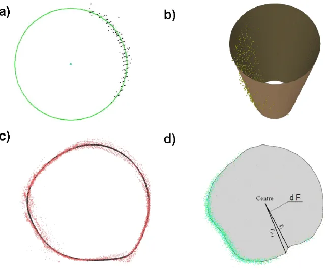
trees (piLine, 2009). Henning and Radtke (2007), and Huang et al (2011) developed automatic object-based registration methods optimized for forest scenes. The algorithms detect point measurements from the stem surfaces in each scan. The stem points were split into 1 m height intervals, which resulted in horizontal stem slice sections. A circle was fitted by least squares adjustment onto each stem slice section. The matching circles were selected upon the similarity in diameter. The orientation parameters were calculated through the ICP algorithm using the corresponding circle centres as input data. This approach resulted in precise image alignments up to approximately 20 meters above the ground, with an average post-registration error of 0.16 cm.

Figure 2-8. Concept of the ICP algorithm illustrated in three iterative steps. (Adapted from Pfeifer, 2007)

The process of georeferencing is similar to that of the registration in the sense it computes the parameters of a congruency transform as well. The indirect solution of georeferencing needs control points with coordinates defined in the superior reference system. The control points are marked in the field with the same type of reflectors as it was mentioned at the tie points. Direct georeferencing can be applied with instruments that have the ability to locate the absolute position, azimuth and inclination of the sensor. The position and attitude of the scanner is measured by a GNSS receiver coupled with biaxial inclination sensor. The azimuth can be estimated by compass or using a pair of GNSS sensors equipped on a fixed base.

Deviation of the stand axis from the vertical, defined by the local gravity field, may be observed and corrected with an electronic spirit level. Although direct georeferencing has the highest degree of automation, it has not come into wide use so far because of its limited accuracy (Berényi, 2011). However, this technique could be convenient for applications in forested areas where surveying base points are usually not available near the scanner position.

2.4. Data structures

2.4.1. Dimensions and data types

Models represent objects with respect to relevant aspects. Our models aimed at describing the components of a forest scene, typically the ground surface and the structure of the vegetation with specific regard to the position, size and shape of the trees.

The expression data type refers to the storage form of the geodata set that can be either regular or irregular. The spatial information content is stored as vector coordinates in case of irregular storage format. Point coordinates have no extent thus the distance between the neighbours can be arbitrary allowing representation of irregular patterns. The regular spatial structure resulted in well-defined neighbourhood relations as the data stored as an array of small cells with identical size and shape. Both data type can have spatial extent in two or three dimensions.

Most of the laser scans are stored with rectangular coordinates in irregular pattern so the primary storage structure of the point cloud is a type of 3D vector. It is convenient to reduce the number of dimensions from three to two by creating a thin horizontal subset where the

(17)

coordinates can be neglected in the course of processing that simplifies the algorithm and saves computational time.

The regular variant of the 2D vector data type is called raster. It is composed by uniform cells of equal spacing with neither overlap nor gap between the adjacent elements. The shape of the cells is squared in far the most cases, however rectangular or hexagonal structures are also possible.

Extending horizontal squared cells in the height domain, the shape of the elements turns to be cubic called voxels (volumetric pixel), while the corresponding 3D grid structure is referred to as voxel space (Figure 2-10). Voxel space can be interpreted as a stack of horizontal rasters of unit height. The inverse of the statement is also apprehensive: Raster is a voxel space of unit height. Regular data composed of squared cells are also named as grid structure in general including rasters and voxel spaces. Grid data can be displayed as digital images (Czimber, 1997).

Grid data are arranged in columns, rows and planes indexed by (i, j,k) non-negative integers. Each cell is located in this grid coordinate system and represented by a digital number. The spatial resolution of the grid is expressed by the cell sized. A point cloud given with vectors of (x,y,z)coordinates can be stored as a grid composed of ni, nj, nk cells, where the symbol

 

refers to the ceil function:



 

 d

x n_i x^max ^min ,



 

 d

y n_j y^max ^min ,



 

 d

z

n_k z^max ^min (2-4)

Figure 2-9. Representation of laser scanned data a) 3D point cloud, b) horizontal subset of stem surface points and c) their representation in a binary raster. (Source data: Hidegvíz-völgy Forest Reserve, Hungary, 2006.

Figure compiled by the author) a)

b) c)

(18)

k j i

j i

k = 0

nk-1 1

nk-2 ...

0 1 ... ni-2 ni-1 i =

nj-1 1

nj-2 ...

j = 0

Figure 2-10. The 3D voxel space is composed of a set of 2D rasters. The cells are identified by the indices of columns (i), rows (j) and planes (k).

In a grid structure, the location of any point measurement is represented by the midpoint of the corresponding cell. If the top back left corner of the grid is georeferenced by (xmin, ymax, zmax) coordinates and the rows have the same orientation as the axis X, the cell indices of an arbitrary point with(x,y,z)coordinates can be calculated by the following formula, where the symbol

 

refers to the floor function:



 

 d

x i x ^min ,



 

 d

y j y^max ,



 

 d

z

k z^max (2-5)

The corresponding relations for calculating the (x,y,z)coordinates from the midpoint of the cell (i,j,k) are as follows:

d i

x

x _min ( 0,5) , y y_max (j0,5)d, zz_max (k0,5)d (2-6) Midpoints of the grid cells retain the original (x,y,z)coordinates with an error of

2 d at the worst case. The absolute error raised as the resultant of coordinate errors is up to

2 d

3 that is reduced to d 2

2 at raster data with the omission of the height component.

Points within the area of a given raster cell (i,j,k) can be queried from the original point cloud, as the corresponding points fulfil the following system:

min

min x (i 1) d x

x d

i       d j y y d j

y_max ( 1)   _max   (2-7)

d k z z d k

z_max( 1)   _max 

The term ‘distance’ of cells (A,B) is generally referred to the Euclidian norm of the cells’

midpoint that is computed by (2-8):

2 2

2 ( ) ( )

)

( _B _A _B _A _B _A

E X X Y Y Z Z

d       . (2-8)

The use of the Euclidian norm in a grid has the disadvantage that the neighbours of a cell sharing common vertex, edge or face are at different distances. Calculating the distance in Manhattan norm is often more convenient, as in this case, all the connected neighbours of a

(19)

Manhattan norm (or city-block distance) of two voxels is computed as (2-9):

A B A B A B

M x x y y z z

d       (2-9)

The use of Manhattan norm has the further advantage that its computation is less complicate because the Manhattan norm of two cells with integer grid coordinates yields always integer result. The set of points that are equidistant in Euclidian norm from a given point are located on a circle, while in Manhattan-norm the points are on a square.

The digital number assigned to a grid cell is interpreted as a specific attribute of the represented space or volumetric element. In the simplest case, the attribute is a binary code expressing the existence or the absence of a laser scanned point measurement within the cell by the constants 1 and 0 respectively. This kind of grid representation considers the location and neighbourhood relations of the point measurements. Extending the domain of binary codes allows for the storage of graduated data. For example, storing the counts of point measurements for each cell resulted in a point density raster, or computing the average of the intensity values per cells resulted in an intensity image. The term range image refers to raster that contain the distances of the scanner position and the closest point measurement within the corresponding grid cells (Figure 2-11) It may be confusing that the term range image was used as synonym expression for the point cloud in earlier studies. The colour of the reflecting surfaces is recorded by digital camera and it can be displayed using RGB code.

Figure 2-11. Range image: range data stored in a raster. Rows and columns represent constant scanner angle values. (Source data: Hidegvíz-völgy Forest Reserve, Hungary, 2006. Image compiled by the author)

(20)

2.4.2. Image objects

The main goal of tree mapping algorithms is to detect point measurements of tree stems in the laser scanned point cloud. This can be achieved based on general geometric features such as shape and size of the point patterns. However, a single vector or a cell is only a primary element in the data set of the reflecting object and alone reveals nothing about its geometric features. To retrieve information on the shape of the objects an extended subgroup of the primary data has to be analysed with special regard to the spatial relations of its elements.

Neighbourhood relations can be defined in straightforward way at grid data structure. A raster cell has four neighbours with common cell side additionally four others at the corners.

A voxel has six neighbours sharing common face; twelve sharing common edge and eight at the corners (Figure 2-12). A set of connected cells with similar values compose region.

Delineation of regions is done according to a homogeneity criterion of cell values. A plenty of homogeneity criterion has been defined in algorithms for segmentation of remotely sensed images (e.g. Benz et al., 2004, Czimber, 2009).

The algorithms introduced in the present thesis process one-bit (‘black and white’) binary grids. Cells containing at least one laser point measurement are coded '1' and called signed (foreground), while the complement set of cells are coded '0' and called empty (background).

A set of signed cells in connection to each other is called region in binary image processing.

Delineation of regions is achieved through Connected Component Labelling algorithms (CCL) that find all regions in an image and assign a unique label to all cells in the same region (Jain et al, 1995). Image objects are regions organized in data structure that ensures unique identification for each region and enables linking attributes. The size of the smallest image object is one cell. Attributes of image objects relate to size, position, shape, and neighbourhood relations that contribute to their thematic classification.

While connected image objects cover one contiguous region of a scene, disconnected image objects can consist of several isolated parts (Figure 2-13). In case of disconnected image objects, the aggregation of single regions contains reasonable meaning; the coherent objects represent one physical object. Image objects can be organized into hierarchic levels, where the totality of all image objects in each level covers the entire scene. This means that all image objects on a lower level are completely contained in exactly one image object of a higher level (Baatz et al, 2004). Objects on higher levels are called aggregations (super objects). Disconnected image objects should be treated as aggregations as they contain multiple continuous regions.

a)

b)

Figure 2-12. Neighbourhood relations of a raster cell (a, b), and of a voxel (d–f).

(21)

Cells Regions Objects Disconnected object

Figure 2-13. Group of binary cells (a), regions (b) and objects with unique labels A,B,C,D and E (c) composing one disconnected image object labelled with F (d).

Regions of connected image objects are the fundamental elements of binary image processing, however connected image objects can further be split to components (sub objects). Soille and Vogt (2008) presented a morphologic segmentation method that can be used for characterising binary patterns with emphasis on connections between their parts. The resulted components are classified to one of the seven categories (core region, islet, loop, bridge, perforation, edge, and branch). All the terms and idioms in relation to object-based image analysis can be extended to 3D grid data.

2.5. Processing concepts

Three main concepts have been outlined in the literature focusing on the topic of modelling trees from terrestrial laser scanner data. The concepts differ in objective (what to be modelled or estimated), scale (number of target trees), and modelling principle (physical or stochastic approach). The border between the concepts is blurred as they overlap some times to each other and there are some transient methods exist.

1. Tree mapping and estimation of attributes on individual level. The main motivations are (1) to find solutions for using TLS as an alternative technique for the automatic retrieval of classic forest inventory parameters and (2) to widen the range of descriptive data that can be used for forest management applications and ecological investigations. The data capture is typically involves several trees e.g. those that are within a forest inventory sample plot. Due to economical reasons, the surveying is often completed from a single vantage point so the algorithm should be able to manage point clouds from single and multiple scanning positions as well. Specific challenges are the filtering of vegetation points and their classification according to the individuals. The biophysical attributes are estimated through relatively simple structural models.

2. Reconstruction of tree structure. Tree models of this kind reveal the architecture of a single tree including the crown structure with high level of details. Tree models have to provide information on (1) the start point and end point of each branch and (2) radii at these points. In addition, topological models account for the branch hierarchy. To ensure complete model, the sample tree is measured from multiple scanning positions.

The field of potential applications involves the reconstruction of especially valuable trees and assessment of tree volume for the improvement of local volume tables. Time series of tree models are non-destructive means for monitoring tree growth thus they suit for the purpose of ecological researches. Other studies have focused on tree models to explain the impacts of the canopy structure on gas and water exchange and

(22)

to improve the existing radiation transfer models (Cote et al., 2009). Due to the realistic structure and high level of details, these models can be utilized in software packages developed for visualization and design.

3. Retrieval of forest stand attributes on plot level. Studies of this approach are addressing the issue of parameter estimation from terrestrial laser scanner data without distinguishing individual trees in the dataset. The models rather describe the spatial distribution of the aggregated mass of wood and leaves throughout the sample space.

The methods used are dominated by stochastic models and aimed at estimation of leaf area index (Henning and Radtke 2006b, Strahler et al. 2008), gap fraction (Danson et al., 2007), and biomass (Ku et al., 2012).

Present dissertation is intended to deal with tree mapping and estimation of tree metrics on individual level. Accordingly, the overview presented in the following subsections is primarily focusing on concept 1. Furthermore, it implies some studies from the field of tree reconstruction (concept 2) that deemed prospective in forestry-related parameter retrieval.

The review is organized according to the main processing steps of the workflow aiming at tree mapping and parameter estimates:

1. Generation of digital terrain model 2. Filtering of irrelevant data

3. Tree detection

4. Derivation of tree models and attributes

a. Diameter and basal area (area of stem cross-section) b. Stem models

c. Tree height d. Crown structure

The input data for tree mapping is practically the registered point cloud without thematic classes. If the map is required to be located in a projection system, the point cloud should be georeferenced. The digital terrain model (DTM) is necessary to make difference of point measurements from the ground and the vegetation, and to transform height coordinates into relative heights above the ground. Commercial software packages are available for the calculation of high quality DTMs that simplifies to filter vegetation points in indirect way as a complement set of terrain points. Point measurements reflected from the low vegetation or resulting from measurement errors are irrelevant from the viewpoint of tree detection, so they should be eliminated through filtering. The filtering can be regarded as a simple classification of points into ‘tree’ and ‘non-tree’ thematic classes. Detection of trees means that all the remaining vegetation points are classified so that only of those reflected from a given tree are assigned in the same class. The classification is primarily based on the spatial arrangement of data points thus the detection is closely related to the creation of a structural model, which is used for locating the position and quantifying the size and shape of the tree. The possibility for the classification of point measurements according to tree species or even species groups is strongly limited. Although Haala (2004) found differences in the point cloud with regard to tree species using fusion of laser scan and digital imagery data, the potential of the technique is hardly enough for practical use. The increasingly spread of full-waveform technique in terrestrial laser scanning is expected to be a step towards the tree species classification. Using the descriptive full-waveform information in relation to the reflectance properties and roughness of the target surface, the automatic retrieval of taxonomic groups or even health conditions seems prospective but needs experimental support. The quantitative description of the target trees is based on the creation of their structural model. The simplest models are

(23)

models is extended in vertical range, stem models and stem metrics are revealed. Tree height can be yielded by finding the tree tops and matching them with the corresponding tree positions. Crown models generally account for the horizontal and vertical extent of the crowns as well as the hierarchic arrangement of branches.

2.6. Generation of digital terrain models

The first step of the workflow is the creation of the digital terrain model (DTM) and the related classification of points according to the reflecting surface as terrain and off-terrain measurements. Many different concepts for filtering terrain points have been proposed so far, and some of them are available in commercial software packages. For convenience, the terrain elevation is regarded as reference surface to normalize the heights of the point cloud. Hereby the heights of the objects located at distinct elevation above the ground become comparative throughout the scene. The DTM quality has primary influence on the subsequent estimation of stem diameters and tree heights. Filtering of terrain points has another aspect namely that off- terrain points are measurements from the vegetation in forested area. In fact, the complement set of terrain points will be used as input data for the detection of trees.

Filtering concepts rely on the hypothesis that points with locally low elevation relative to their neighbours are reflected from the ground because the laser light is unable to penetrate below the terrain surface. The methods used in wide range of practice have been developed for processing airborne laser scanner data; however, with some modification of their parameters they are appropriate for TLS data as well.

The most frequently used filtering concepts for DTM generation over forested areas from TLS data can be divided into three groups:

1. Filtering based on adaptive threshold 2. Progressive TIN densification

3. Surface interpolation of weighted points.

The earlier filtering methods calculate a threshold on the height coordinates upon which the actual point is either accepted or rejected as a terrain point. Basic variants of these procedures can be implemented through short scripts written in mathematical program packages. The efficiency of the adaptive thresholding is restricted by sharp edges and discontinuity of terrain points. Block minimum filters use a moving horizontal plane with a corresponding upper buffer zone that defines a region in 3D space where terrain points are expected to reside. The plane is located at points with locally the lowest elevation. Points above the buffer zone are deemed off-terrain points. The thickness of the buffer zone is needed as input data, but some more sophisticated routines consider the histogram of elevations and calculate it automatically. A structure element, describing admissible height differences depending on horizontal distance is used at morphologic filtering. The smaller the distance between a ground point and its neighbouring points, the less height difference is accepted between them. This structure element is placed at each point so off-terrain points are identified as those above the admissible height difference. The structure element itself could be determined from terrain training data. For steeper areas, higher admissible height differences are allowed (Vosselman, 2000).

The second group of filters works progressively, where more and more points are classified as ground points. The classical routine of progressive TIN densification starts by selecting some local low points as sure hits on the ground. The algorithm assumes that any areas bigger than the expected largest building have at least one hit on the ground and that the

(24)

lowest point is a ground hit. An initial model from selected low points is created. Triangles in this initial model are mostly below the ground with only the vertices touching ground. The routine then starts refining the model upwards by iteratively adding new laser points to it.

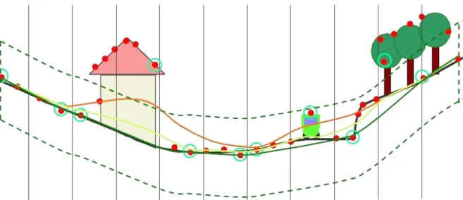
Each added point makes the model follow the ground surface more closely. Iteration parameters determine how close a point must be to a triangle plane so that the point can be accepted to the model. Iteration angle is the maximum angle between point, its projection on triangle plane and closest triangle vertex (Figure 2-14). Iteration distance parameter makes sure that the iteration does not make big jumps upwards when triangles are large. This helps to keep low buildings out of the model (Axelson, 2000, Soininen, 2005).

Figure 2-14. Progressive TIN densification (Mandelburger, 2005).

The third group of algorithms is based on a surface model that iteratively approaches the ground surface through the recalculation of weights for each point according to its height difference relative to the model. The algorithm Robust Filtering computes the surface with equal weights for all points (for all z-measurements) in the first step (Kraus and Pfeifer, 1998). This surface runs in an averaging way between terrain points and vegetation points.

The terrain points are more likely to have negative residuals, whereas the vegetation points are more likely to have small negative or positive residuals. These residuals are used to compute weights for each measurement (Figure 2-15). Now, the weights can be used for the next computation (iteration) of the surface. Points with large negative residuals have maximum weights and they attract the computed surface, whereas points with medium residuals have smaller weights and less influence on the computed surface. This algorithm has been implemented within the program package SCOP++. In SCOP++, the surface is computed by subdividing it into several patches. By doing so, parameters of the weight function are set in an adaptive way for each patch. The method has been embedded in a hierarchical approach to handle extended gaps in terrain data resulted from dense vegetation or large buildings (Figure 2-16).

p

Z 0

Figure 2-15. Weight function for filtering terrain points.(Kraus and Pfeifer, 1998)

(25)

Figure 2-16. Iterative refinement of the ground surface by weighted points (Mandelburger, 2005).

The concept of Active Contours (Snakes) has its roots in the digital image processing. In general, the shape of an active contour is the solution of parameterization that minimizes an energy function that includes internal energy and a potential field. The internal energy is described using physical characteristics associated with the contour, usually material properties like elasticity and rigidity. The potential field is given by the height data. The contour used in this case acts like a sticky rubber cloth or a rubber band net that is being pulled upwards from underneath. The net is attracted by the height data points and sticks to points that are assumed to represent the true ground. The elasticity forces in the rubber band stops the net from reaching points not representing the true ground. The solution is a net that forms a continuous model of the ground surface (Elmqvist et al. 2001). Weinacker et al.

(2004) modified the concept to work in hierarchic manner and implemented in software TreesVis.

2.7. Filtering of irrelevant data

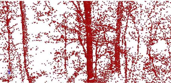
The shape of the trees can be visually identified in the point cloud, although the stem surface points are surrounded by measurements of irregular pattern (Figure 2-17). Some of the scattered data are caused by range finding errors e.g. phase ambiguity or multiple echoes generated by partial interception. The remaining points around the trees are reflected from small or thin components of vegetation for example leaves and twigs. Due to the sparse point density relative to their extent, these reflecting objects can be interpreted neither visual nor automatic manner. Measurements from unidentifiable objects are regarded as irrelevant from the viewpoint of tree detection. Considering the irregular pattern and sparse arrangement, these measurements appear isolated especially as they are usually single points or small group of points relative afar from the stem surface points. Isolated data come into view as speckles in regular data structure. In the presence of thick undergrowth, the ratio of isolated points can exceed the ratio of stem surface measurements that may cause the failure of standard object detection techniques. Their filtering is necessary for automatic tree detection but it facilitates the visual interpretation of forest stands as well.

Points reflected from beyond the efficient ranging distance of phase-shift-based instruments appear as if they were within the ambiguity interval. Actually, these ghost points are reflected from afar so their intensity values are lower than those are of the surface points within the effective range. Ghost points from multiple echoes have alike lower intensity because of the smaller area of reflection.

(26)

Figure 2-17. Stem surface points with significant amount of data reflected from other vegetation components.

(Source data: Pro Silva demonstration site, Pilis, Hungary, 2006. Figure compiled by the author.)

Filtering ghost points can be achieved by thresholding the minimum intensity value.

Schilling et al. (2011) found this technique effective, as it reduced the point number by 15–

29% in advance a tree modelling procedure. According to the experience of Simonse et al (2003), natural objects never have high intensity values. This means that a very high intensity also indicates data noise when measuring in forest stands. Twigs and leaves reflect only a few laser measurements resulted in isolated points or small group of points being relative afar from their neighbours. A single point can be removed if it does not have enough neighbour within a given search radius. Due to the viewing geometry, the search radius should be increased with respect to the distance from the sensor. A commonly used gridding technique for the elimination of isolated points is to fill only the cells of those that contain point counts exceeding a given minimum value. Aschoff and Spiecker (2004) mapped the horizontal section of the point cloud into a point count raster and removed isolated points by adaptive thresholding of the minimum cell values. The routine considered the number of surveying points and summarized the potential point counts for each cell. Gorte and Pfeifer (2004) defined neighbourhood operations and filtering rules on object size (i.e. minimum cell counts) to remove isolated cells from the voxel space. Simonse et al. (2003) proposed filtering for range images assuming that neighbouring cells contain point measurements with similar distances. If a cell value extremely deviates from the value of its neighbours, it represents isolated data.

Specific filtering is needed to remove point measurements reflected from branches for the estimation of stem diameter. This holds high importance especially at conifers where dead branches remain on the lower part of the bole. As branch points are often arranged into sparse groups of linear or amorphous pattern, their local context has to be also considered. Bienert et al. (2007) developed a filtering routine for point count rasters to separate point measurements from the bole and from the branches. It can be used for single scan data knowing the nominal scan resolution and scanning position. Assuming regular scanning pattern, the theoretical maximum of point measurements can be calculated for each cell by summing up the laser beams passing through the region of the cell. Comparing the maximum and the actual point counts, cells below a distinct value were assumed to contain smaller objects then the cell size and were treated as irrelevant speckles (Figure 2-18).