1
Modular analysis of brain and free word association networks
PhD Dissertation
Bálint File
Scientific advisor:
Dr István Ulbert DSc
Roska Tamás Doctoral School of Sciences and Technology Faculty of Information Technology and Bionics
Pázmány Péter Catholic University
Budapest, 2019
2
T ABLE OF C ONTENTS
1 Abstract... 9
2 Measuring the influence of a node in the formation of the functional brain modular organization ... 10
2.1 Introduction ... 10
2.2 Methods ... 12
2.2.1 Participants ... 12
2.2.2 Modularity and partition distance ... 13
2.2.3 Comparison of the local modularity to the within-module connectivity and participation coefficient value. ... 15
2.2.4 Statistical evaluation ... 16
2.3 Results ... 17
2.3.1 Modularity and partition distance ... 17
2.3.2 Age-related local modularity changes of brain networks ... 18
2.3.3 dQ values of the approximation node shifts ... 20
2.4 Discussion ... 21
3 Scale free and modular network properties can describe the organization of a free word association network ... 23
3.1 Introduction ... 23
3.1.1 Heroism ... 23
3.1.2 Social representations ... 24
3.1.3 Networks ... 25
3.2 Material and Methods ... 26
3.2.1 Participants ... 26
3.2.2 Measures ... 26
3.2.3 Setting up the networks ... 27
3.2.4 Scale-free topology and modularity... 29
3.2.5 Normalization of node strengths ... 30
3.3 Results ... 31
3.3.1 Structural differences of the common associations ... 36
3.4 Discussion ... 38
4 The modular investigation of free word association network can reveal polarized opinions 39 4.1 Introduction ... 39
4.1.1 Method demonstration: Public opinion of “migrants” ... 40
4.1.2 Research goals and validation process ... 41
4.2 Methods ... 42
3
4.2.1 Participants and procedure ... 42
4.2.2 Measures ... 43
4.2.3 Preprocessing of associations ... 45
4.2.4 CoOp Network Construction ... 46
4.2.5 Affective Similarity ... 47
4.2.6 Module Detection ... 47
4.2.7 Testing robustness ... 48
4.2.8 Statistical analysis... 50
4.3 Results ... 51
4.3.1 CoOp Connections and Affective Similarity (Hypothesis 1) ... 52
4.3.2 CoOp Modules ... 54
4.3.3 CoOp Modules and POT scores (Hypothesis 2) ... 55
4.3.4 Robustness (Hypothesis 3) ... 58
4.4 Discussion ... 59
5 Summary ... 65
5.1 Thesis group I. Application of the modularity value on local scale in functional brain networks ... 65
5.2 Thesis group II. Modular investigation of free word association networks ... 66
6 The author’s publications ... 67
6.1 Publications related to the present thesis ... 67
6.1.1 Papers: ... 67
6.1.2 Oral presentations: ... 68
6.1.3 Poster presentations: ... 68
6.2 Publications not related to the present thesis ... 68
6.2.1 Papers: ... 68
6.2.2 Oral presentations: ... 69
6.2.3 Poster presentations: ... 69
7 Acknowledgements ... 70
8 Bibliography ... 71
4
List of abbreviations
Q: modularity value
fMRI: functional magnetic resonance imaging N: Sample size
SD: standard deviation TR: repetition time TE: echo time
FA: fractional anisotropy
FWHM: Gaussian smoothing kernel with a full width at half maximum ROI: region of interest
FSL: comprehensive library of analysis tools for FMRI MIn: normalized mutual information
DMN: default mode network dQ: delta modularity value
dMIn: delta normalized mutual information r: Pearson’s correlation coefficient
p: probability value
CoOp networks: networks of co-occurring opinions QAP: quadratic assignment procedure
LLR: Log-likelihood Ratio POT: Perceived Outgroup Threat GM: Group Malleability
SDO: Social Dominance Orientation M: mean
WAM: Weighted attitude score means WAV: Weighted attitude score variance rs: Spearman’s correlation coefficient
PANAS: Positive and Negative Affect Schedule
5
List of figures
Figure 2.1. Representative modular organization of young (A) and elderly (B) groups. Different node colors denote different modules. The coloring of the modules was optimized by the Hungarian algorithm [1] using Jaccard-similarity between the modules as a cost.
Figure 2.2. Age-related differences in local modularity. The local modularity determines the correspondence of a given node to the modular organization of a network. The spheres denote brain regions which show a significantly higher (p<0.05) local modularity (segregation) in the young (A) and elderly (B) representative community structure. Spheres with larger radius mark p<0.01 level of significance. Color marks the modules in a similar fashion as in Figure 2.1.
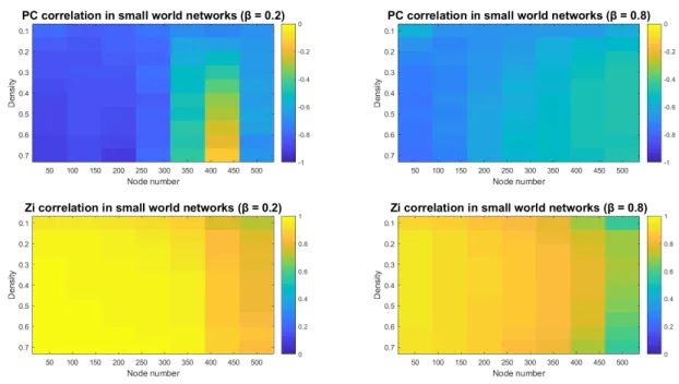
Figure 2.3. Correlation between „local modularity” and „participation coefficient (PC)/within module connectivity (Z)” on simulated networks. Small-world networks were generated with different node numbers and density. The rewiring probability (β) was set to 0.2 for a lattice like network and 0.8 for simulated random networks. The heatmaps represent the correlation values.
The correlation values were the following: PClattice(-0.7047±0.1891) Zlattice (0.9282±0.07);
PCrandom (-0.6055±0.09), Zrandom(0.8316±0.09
Figure 3.1. Scale-free properties of the Hero (A) and Everyday Hero (B) networks. The plots show the cumulative distribution functions of the normalized node strengths on log-log scales.
The dashed, straight lines represent the Maximum Likelihood Estimation fitting of the data points. The power law exponents (α) for the Hero and Everyday Hero networks are 2.15 and 2.21, respectively.
Figure 3.2. The modularity values of the Hero (left) and Everyday Hero (right) networks comparing to the null models. The error bars refer to the standard deviation of the modularity value derived from the null models. The modularity value of the Hero network (Q=.19) was not significantly higher than the corresponding modularity values of the null models suggesting a cohesive representation. The modularity value of the Everyday Hero network (Q=.27) was
6
significantly higher than the modularity values of the null models referring to multiple socio- cognitive categories.
Figure 3.3. The social representations of Hero (A) and Everyday Hero (B). The association networks are visualized with the ForceAtlas 2 layout. The size of a node denotes the node strength and the thickness of an edge refers to the edge weight. The networks were thresholded (edges below the value of 1 were deleted) for a better visualization. In case of Everyday Hero, nodes with the same color belong to the same module. The hierarchy and descriptive labels of the modules are presented on the dendrogram.
Figure 3.4. Common associations in the social representations of Hero (A) and Everyday Hero (B). The associations are arranged in a circular alphabetic order. The size of a node denotes the node strength and the thickness of an edge refers to the edge weight. The network was thresholded (edges below the value of 1 were deleted) for a better visualization.
Figure 4.1. Correlation between affective similarity values and co-occurrence connections (A) and correlation between the identical co-occurrence connections in Sample1 and Sample 2 (B).
(A) The x-axis shows the co-occurrence connection values and the y-axis shows the affective similarity values. The x-coordinates of the data points represent the averages of the co- occurrence connection values in each of the 100 equal intervals. The association pairs were determined in each interval and their affective similarity values were also averaged. The y- coordinates of the data points represent these averaged affective similarity values. (B) The similarity of the co-occurrence connections between identical associations in the two samples was measured by Spearman’s correlation. The x-axis shows the co-occurrence connections in Sample 1 and the y-axis shows the co-occurrence connections in Sample 2.
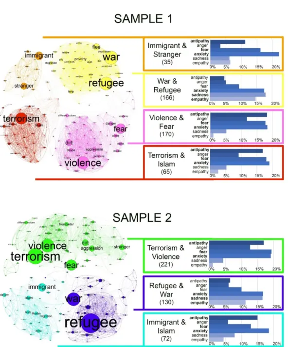
Figure 4.2. The modules of the CoOp networks. Each module is visualized with different colors.
The size of a node and its label is proportional to the frequency of the given association. An edge means that two associations fall into a common module in the consensus partitioning procedure at least 40%. Both sample is displayed by “Yifan Hu Proportional” layout algorithm
7
[2] implemented in Gephi [3]. Additional information about each module is shown in a box colored identically to the corresponding module. The box contains the label of the module referring to the two most frequent associations in a given module. The number of respondents assigned to a given module is displayed below the label in parentheses. The percentages of emotional labels for every module are presented on bar charts. The percentage of the six most frequent emotions (antipathy, anger, fear, anxiety, sadness, empathy) are shown in detail. The three most frequent emotions are displayed with bold letters.
Figure 4.3. Perceived Outgroup Threat (POT), Group Malleability (GM) and Social Dominance Orientation (SDO) scores of the modules in Sample 1 and Sample 2. Bars represent the mean of the POT = Perceived Outgroup Threat, GM = Group Malleability and SDO = Social Dominance Orientation scores for every module. Standard error was presented on the bars. All pairwise comparisons of the modules showed significant differences in POT scores. See detailed POT analysis results below.
Figure 4.4. Correlation between the reliability and the exclusion of rare associations from the analysis. The x-axis shows the minimal number of occurrence of an association. Below that occurrence number, an association was excluded from the analysis. The y-axis shows the LLR (correlation) and modular (nMI) level similarity between the randomly divided samples. Error bars represents the standard deviation of the 100 independent runs. Exclusion of rare associations was resulted in higher LLR similarity and higher modular similarity in Sample 1 and Sample 2.
List of tables
Table 3.1. Global hubs of the Hero and Everyday Hero networks. Normalized node strength >
2.5 refers to the global hubs of the association network.
8
Table 3.2. Modular hubs of Everyday Hero network. Normalized node strength > 2.5 refers to the modular hubs of the association network.
9
1 A BSTRACT
Networks are used for exploring underlying relations in various datasets by defining nodes and edges corresponding to a certain logic of the observed system. In the recent decades, numerous parameters were developed to describe different properties of the networks. Modular organization is an important topological property, in which certain group of nodes have denser connectivity within themselves than between other regions of the network. Also the nodes constituting a given module probably share similar properties regarding the analyzed phenomenon. Modularity maximization is among the most popular network modularization algorithms, hence the number and size of the modules are not predefined. In the present thesis 1) I demonstrated a modularity value based improvement for the statistical evaluation of brain networks and 2) I developed and validated a process for defining polarized opinions based on the modules of free word association networks.
The statistical evaluation of brain networks is based on measuring the decrease of modularity caused by shifting a node from its own module to another module. On one hand, local modularity measures the influence of a node in the formation of the modular organization.
On the other hand, we evaluated differences in the community membership of the nodes between the modular structures of two groups. The method was tested on resting-state fMRI data of 20 young and 20 elderly subjects. The findings indicate that applying the modularity on a local scale is a promising biomarker for detecting differences between subpopulations.
We developed a method which can identify polarized public opinions by finding the maximal modularity partitioning in a network of statistically-related free word associations. The co-occurrence based relations of free word associations reflected emotional similarity and the modules of the association network were validated on well-established measures. The results were relatively consistent in two independent samples. We demonstrated that analyzing the modular organization of association networks can be a tool for identifying the most important dimensions of public opinions about a relevant social issue without using pre-defined constructs.
10
2 M EASURING THE INFLUENCE OF A NODE IN THE FORMATION OF THE FUNCTIONAL BRAIN MODULAR ORGANIZATION
2.1 I
NTRODUCTIONGraph theoretical analyses of complex functional networks, obtained using fMRI and MEG (for review see [4]), has demonstrated that brain functional networks have a modular (sub- network) structure, where a module is defined as a highly integrated sub-network consisting of regions with much denser connectivity among themselves than between those regions and the rest of the brain. Importantly, it has been shown that these modules are mainly composed of brain regions which are functionally and anatomically related to each other [5]. In general, integration within a module allows efficient local processing, while segregation between modules may be necessary to avoid interference from internal or external noise that could interfere with function of the modules neural activity. Therefore, studies of brain modules enable the identification of groups of brain regions that may serve common cognitive functions of neural activity [6]. Alterations of the global functional modular structure and decreased efficiency of the modular hub regions are observed in clinical and non-clinical states [7]–[9].
Although there is not a universal way for detecting the community structure in complex networks, the modularity (Q) value optimizing algorithms [10] became the gold standard for identifying the functional brain modules. The modular partition of a network with the highest Q value comprises many within-module links and as few as possible between-module links.
Modules of within a complex network can be organized in various ways. A homogenous degree distribution among a module provides equivalent importance of the nodes, while a hierarchical structure of modules establishes nodes with a higher centrality than others [11]. The aim of the current study was to present a method to evaluate differences in the community membership of the nodes between representative modular structures.
Representative community structures are derived from multiple subjects of a single clinical sample, or condition, thus it gives a unique, characteristic modular organization. The
11
visual demonstration of different representative modular structures is hardly accompanied with their statistical evaluation. On one hand, the comparison of two, unique networks are not trivial, on the other hand, the non-linear nature of the community detection algorithms makes extremely difficult to statistically evaluate certain visual differences. For example, how can we prove that the merging of two modules have a higher impact on the differences between two representative modular structures than the altered community assignment of one single node? Considerable visual differences between representative modular structures may originate in the altered connections of a single node, which restructure the whole community structure.
During the recent years graph theoretical measurements were developed to define the differences in community assignments of brain regions between the two subpopulations [12], [13]. The consistency of the modular structure across subjects is measured by the scaled inclusivity [13], and the modular classification of a particular brain region can be detected by Pearson’s phi [12]. These methods work with the labels of the modular assignment corresponding to the maximal modularity partitioning. The label assignment is a binary process:
a node is included or excluded from a community, however it is clear, that changes of the partition label of certain brain regions influence the modular organization more, than other do.
Our method is based on the quantification of the decrease of the modularity caused by shifting a node from its own module to another module. Measuring the extent of the modularity decrease caused by changing the community membership for every node, highlights nodes which are playing more important role in the maintenance of the modular structure. We also applied the method to identify significant differences in the modular assignment of the nodes between the representative community structures of two samples. We defined nodes whose community membership changes approximate the modular structure of one sample towards the other. A node with a community membership change was considered as approximating one community structure toward the other if the distance between the original community structures decreased by changing the community membership of the node. The modularity decrease caused by the approximation process was evaluated with a permutation framework. Applying the
12
technique, we could pinpoint certain nodes (brain regions), for which community membership is prominently different in the community structure in one sample, compared to that seen in the other.
We tested the method on resting-state fMRI data of young and elderly subjects. The elderly functional network was characterized by altered community structure [14], [15] reduced modularity [14] and generally more between-module and less within-module connections than the young network [16]. We expected that our method can detect the prominent regions whose modular memberships are crucial for the formation of the young and elderly brain networks.
2.2 M
ETHODS 2.2.1 ParticipantsData of healthy young (19-21 years; N = 20; SD= ±1; 9 women) and elderly (67-85 years; N = 20; SD= ±6; 10 women) individuals was analyzed in this study. fMRI data was obtained from the ‘INDI NKI/Rockland Sample’. fMRI time series from each participant were acquired in eyes open resting state condition during a 11 minutes period.
fMRI recording, preprocessing and functional connectivity assessment
All subjects were scanned with the same scanner (MRC35390 SIEMENS TrioTim 3T, TR=2500=ms, TE=30 ms, FA=80°, 3x3x3 mm voxels, 260 frames).
Preprocessing steps were carried out by using SPM12 and Conn 15d toolboxes. Default preprocessing steps were applied with default parameters in Conn: (1) realignment, (2) slice- timing correction, (3) segmentation and normalization, (4) ART-based scrubbing, (5) smoothing using a 8 mm full-width half-maximum (FWHM) Gaussian kernel. After the preprocessing steps the fMRI time series were band-pass filtered ([0.008 0.09] Hz), white matter and cerebrospinal fluid time series were regressed out. 95 ROIs (cortical areas and the hippocampus) were determined applying the FSL Harvard-Oxford Atlas parcellation scheme [17]. Regional average time courses of the ROIs were extracted for each individual.
13
Pairwise temporal correlations between all ROIs’ time series were calculated, and used as measures of connectivity strengths. Correlation coefficients were converted into z-values using Fisher’s transformation. Because of the ambiguity regarding the meaning of negative correlations [18], negative z-values were set to zero in the connectivity matrix. The connectivity strengths of every participant was normalized between 0 and 1. Normalization was done by a linear function, which does not affect individual network properties, but avoiding the possible bias of the inter-subject connectivity strength variance [19].
Every subject was characterized by a weighted, undirected network, where the ROIs represented the nodes and the connectivity strengths defined the weights of edges. The representative modular structures were derived from the average connectivity network [15].
2.2.2 Modularity and partition distance
In order to determine the modular structure, smaller functional subgraphs or modules were decomposed from the entire resting state network. The modularity (Q) of a graph describes the possible formation of communities in the network:
,
where N is the number of modules, L is the total sum of all edge weights in the network, ks is the sum of all weights in module s, and ds is the sum of the strength of nodes (the sum of edge weights of a certain node) in module s [10]. The Louvain algorithm [20] was applied to identify modular partition with high modularity. The representative modular structure was determined by applying the modularity algorithm on the young and elderly subjects’ average connectivity matrices respectively.
The distance between different partition representations of networks with identical nodes can be determined by the normalized mutual information (MIn):
𝑀𝐼𝑛 = 2 ∗𝐻(𝑌) + 𝐻(𝐸) − 𝐻(𝑌, 𝐸) 𝐻(𝑌) + 𝐻(𝐸)
14
where H(Y) and H(E) is the entropy of the young and elderly partitions respectively and H(Y,E) is the joint entropy of the two partitions [21].
Local modularity and approximation node shifts
The relative importance of each region in the maintenance of the modular organization was measured by shifting each brain region to all possible extraneous modules. Shifting a node with an unstable community membership has less effect on the modularity value than shifting a node from its unique group [19]. Each transformation can be characterized by the change of the modularity value:
𝑑𝑄𝑖 = 𝑄𝑏𝑒𝑓𝑜𝑟𝑒 𝑡𝑟𝑎𝑛𝑠𝑓𝑜𝑟𝑚𝑎𝑡𝑖𝑜𝑛 𝑜𝑓 𝑛𝑜𝑑𝑒 𝑖 − 𝑄𝑎𝑓𝑡𝑒𝑟 𝑡𝑟𝑎𝑛𝑠𝑓𝑜𝑟𝑚𝑎𝑡𝑖𝑜𝑛 𝑜𝑓 𝑛𝑜𝑑𝑒 𝑖
The average value of 𝑑𝑄𝑖 is the local modularity for node i. It defines how strongly the node is connected to its own module. The local modularity value can also be interpreted as the correspondence of a given node to the modular organization of a network.
Beside the calculation of the local modularity we can mark certain node shifts between modules, which approximate one partition towards the other (approximation node shifts). The changes of the MIn (dMIn) can detect these node shifts:
𝑑𝑀𝐼𝑛 = 𝑀𝐼𝑛(𝑦𝑜𝑢𝑛𝑔, 𝑒𝑙𝑑𝑒𝑟𝑙𝑦) − 𝑀𝐼𝑛(𝑦𝑜𝑢𝑛𝑔′, 𝑒𝑙𝑑𝑒𝑟𝑙𝑦),
in which dMIn values with negative sign denote node shifts, which approximate the young partition towards the elderly.
It is important to emphasize that the presented analysis is not symmetric, thus the two age groups have different representative partitions. Therefore, it is necessary to perform it on the calculated networks both for the young and the elderly separately.
15
2.2.3 Comparison of the local modularity to the within-module connectivity and participation coefficient value.
In order to test the relation between the local modularity and other well-known network measures random networks were generated. Small-world networks (binary, undirected) were generated with different edge density (from 0.1 to 0.7 with 0.1 steps) and with different node numbers (100 to 500 with 50 steps). The rewiring probability was set to 0.2 and 0.8 in order to generate lattice like random networks (rewiring probability = 0.2) and random networks close to the Erdős-Rényi graphs (rewiring probability = 0.8) [22]. 100, independent, random networks were generated with each parameter set. The resulted networks modularized in the same way than described for the biological networks. For every network the modular role of each node was characterized by the local modularity and two additional measures: within-module connectivity and participation coefficient.
Within-module connectivity (Z) measures the overall connectivity of the node (its strength) within the module compared to that of the other nodes in the same module:
𝑍𝑖 =𝐾𝑖−〈𝐾𝑆𝑖〉
𝜎𝑆𝑖𝐾 ,
where Ki is the within-module strength of node i (sum of all edge weights between node i and all the other nodes in its own module, Si), 〈𝐾𝑆𝑖〉 is the average of the within-module strength for all nodes in module Si, and 𝜎𝑆𝐾𝑖 is the standard deviation of K in module Si [11].
The participation coefficient (PC) of a node refers to the level of “between-modular”
connectivity strength expresses how strongly a node is connected to other modules and defined as:
𝑃𝐶𝑖 = 1 − ∑ (𝑊𝑖𝑠 𝑊𝑖)
𝑁 2
𝑠=1
16
where N is the number of modules, 𝑊𝑖𝑠 the summation of edge weights of node i to module s and 𝑊𝑖 is the weighted degree of node i (Guimera and Amaral, 2005).
For each network Pearson’s correlation was calculated between the local modularity and participation coefficient and between the local modularity and within-module connectivity values of the nodes.
The local modularity values of the representative brain networks of the two age groups were also compared to the PC and Z values.
2.2.4 Statistical evaluation
Modularity values of the two age groups were compared using a permutation procedure. In each step an average network of mixed group was created by randomly exchanging the membership of young and elderly subjects, then the maximal modularity value for this mixed group was calculated. Repeating the procedure 5000 times, we could fit the original young and elderly modularity values to the distribution of the mixed groups’ maximal modularity.
The level of significance of the local modularity of every node and the approximation node shifts were also determined with the distribution provided by mixed groups. The young and elderly modular partitions showed a different pattern of node assignment to modules, thus we tested them separately.
For describing the process, we chose the young group as a reference. The nodes of the mixed group average network were assigned to the same modules as the young representative partition.
The local modularity of each node and the dQ caused by the approximation node shifts were determined. Since the mixed group was divided into the same modules as the young group, the same approximation node shifts were applied to the mixed group as to the reference group.
Repeating the procedure for 5000 times we got distributions for the local modularity and for the dQ of every approximation node shifts. The null hypothesis was rejected if the local modularity (or dQ of a particular approximation node shift) of the reference group was lower than 95% of
17
the corresponding value of the mixed group. The null hypothesis was tested for every local modularity value and for the dQ of every approximation node shifts separately.
2.3 R
ESULTS2.3.1 Modularity and partition distance
The modularity of the young representative network (Qyoung=0.25) was significantly higher than that of the mixed group (p=0.0036, 5000 permutations), while the modularity of the elderly representative network (Qelderly=0.21) was significantly lower than that of the mixed group (p=0.016, 5000 permutations).
The modularity algorithm detected 4 functional modules in the young and 3 modules in the elderly group (Figure 2.1.). The occipital module showed the highest overlap between the two age groups, while the fronto-temporal and the default mode network (DMN) were merged to one single cluster in the elderly group.
18
Figure 2.1. Representative modular organization of young (A) and elderly (B) groups. Different node colors denote different modules. The coloring of the modules was optimized by the Hungarian algorithm [1] using Jaccard-similarity between the modules as a cost.
We checked whether the modularity differences can be related to the different network density of the two age group. We have not found any significant differences in the density:
DensityYoung=.84±.05; DensityEldelry=.85±.05; t(38)=-0.66, p=0.5.
2.3.2 Age-related local modularity changes of brain networks
As the young group was characterized by a significantly higher modularity than the elderly group, the higher local modularity values were also found in this group (Figure 2.2.).
The most prominent increase of the local modularity in the young group compared to the mixed group was observed in the occipital regions (15 from the 18 occipital regions showed significantly higher local modularity). On the contrary, the local modularity of the structures of
19
the default mode network was only slightly affected by aging. Increased local modularity was found only for 4 (right/left hippocampus, left parahippocampal gyrus, left angular gyrus) of the 13 regions of the DMN.
In contrast to the young group only a few regions of increased local modularity were observed in the elderly group. The medial frontal cortex (p=0.03), paracingulate gyri (pright=0.03; pleft=0.001), superior parietal lobules (pright=0.009; pleft=0.01) and inferior temporal gyri (pright=0.004; pleft=0.05) showed an increased local modularity compared to the mixed group.
Figure 2.2. Age-related differences in local modularity. The local modularity determines the correspondence of a given node to the modular organization of a network. The spheres denote brain regions which show a significantly higher (p<0.05) local modularity (segregation) in the young (A) and elderly (B) representative community structure. Spheres with larger radius mark p<0.01 level of significance. Color marks the modules in a similar fashion as in Figure 2.1.
Local modularity values were compared to the Z and PC values of simulated small-world networks with different parameters and also to the young and elderly networks, For the
20
biological networks, the local modularity value showed a moderate to strong negative correlation with the PC values (PCYoung= -0.93, PCEldelry= -0.65) and the same strength but different direction with the Z values (ZYoung= 0.74, ZEldelry= 0.9). We obtained a similar result for the simulated small-world networks (for detailed results, please see Figure 2.3).
Figure 2.3. Correlation between „local modularity” and „participation coefficient (PC)/within module connectivity (Z)” on simulated networks. Small-world networks were generated with different node numbers and density. The rewiring probability (β) was set to 0.2 for a lattice like network and 0.8 for simulating random networks. The heatmaps represent the correlation values. The correlation values were the following: PClattice(-0.7047±0.1891) Zlattice (0.9282±0.07); PCrandom (-0.6055±0.09), Zrandom(0.8316±0.09).
2.3.3 dQ values of the approximation node shifts
There were 28 approximation node shifts from the young group toward the elderly, and 9 approximation node shifts from the elderly group toward the young. In case of the young group node transformations indicated shifts mainly from the fronto-temporal module, since this module was absorbed to other modules in the elderly group (see Figure 2.1.). The majority of the approximation node shifts caused a significant modularity decrease compared to the mixed group.
In case of the elderly, transformation of the bilateral middle temporal gyri (pright=0.05;
pleft=0.05) and the right supramarginal gyrus (p=0.045) from the ‘centro-parieto-temporal’
21
module to the ‘fronto-temporal + DMN’ module resulted in a significant modularity decrease compared to the mixed age group. Changing of the modular assignment of the bilateral superior parietal lobules (pright=0.02; pleft=0.04) from the elderly group’s ‘centro-parieto-temporal’ to the young group’s ‘occipital’ module also resulted in a significant modularity decrease compared to the mixed age group.
2.4 D
ISCUSSIONThis work introduced a novel method for investigating modularity on a local scale. The method is based on the quantification of the modularity decrease caused by changing the community membership of the nodes. Our novel measure, local modularity, reveals the influence of a node’s community membership in the modular organization of a network. We also defined nodes whose community membership changes approximate the modular structure of one sample towards the other. Measuring the modularity decrease caused by these node shifts pinpointed certain nodes community membership of which were prominently different in the community structure in one sample than in the other. The resulting modularity of the node shifting was statistically evaluated with a permutation framework.
We tested the method on resting state fMRI data of young and elderly subjects. As far as we know, this is the first attempt to apply modularity in a nodal scale for investigating the differences between functional brain networks. The local modularity is positively related to the within module connectivity and negatively to the between module connectivity thus nodes with high local modularity value can be related to local hubs (nodes with high within module connectivity and low participation coefficient) of the network[23].
We identified 4 modules in the young and 3 in the elderly group. The same number of resting state functional modules were described previously, however more sparse networks can result in more modules [15]. Similarly to other findings [14], [16] we found increased modularity in the young group. The highest local modularity was observed in the occipital module of the young group. This observation is in line with the increased segregation of the
22
visual cortex in the young [14]. Increased local modularity in the elderly was mainly observed within the regions of the dorsal attention network (prefrontal cortex, anterior cingulate, posterior parietal lobule), indicating that these regions may preserve the modular organization of the brain network in advanced age. In a previous study it was found that the long range connections within this system showed an age-related decrease [24]. Probably the disconnection of the network resulted in the increase of local modularity.
We found the merging of the DMN to the ‘fronto-temporal’ module in the elderly group.
Our method showed that the changes of the community assignment of these regions have a significant impact on the modularity. Geerlings and his colleagues found using the labels of the partitions [14], that the DMN only create a separate module in the young group, but merges with the fronto-parietal control network with advanced age. Also a very recent study confirmed that the between module connections of the fronto-parietal control network increased with age [25].The present findings indicate, that modularity estimated on a local scale can be a promising parameter for measuring the influence of a node in the formation of the modular organization of a network and to detect changes of the community memberships between different groups.
Future studies may extend the application of the local modularity and approximation node shifts.
Local modularity can be applied on any network to measure the relative importance of each node. Approximation node shifts has three criteria for application: 1) comparison of two, or more conditions, 2) more observation within homogenous groups 3) networks with equivalent nodes.
Beside the comparison of brain networks, approximation node shift may be used for filtering noise from multiple observations.
As a limitation of this study we have to refer to the thresholding problem of functional brain networks. We used a biologically relevant cut-off values [18], [26] and from a practical view, the positive edges ensure a better partitioning of the functional network than the negative edges [19]. Moreover, age-related changes of the fMRI modular organization investigated only positive edge weight networks, thus for a better comparison to the current literature [14], [15], [27], [28] we applied the common practice. Besides this, we have to acknowledge that choosing
23
a threshold is always an arbitrary choice [29]. Similarly, choosing the number of nodes in our network (i.e. the number of brain regions in the Harvard-Oxford parcellation scheme) can have an effect on the modular structure of the network [30]. Changing the community memberships of a partition was limited to individual node shifts between communities in this study, however applying more sophisticated transformation rules (e.g: merging, splitting partitions) may improve the sensitivity of the method in the future.
3 S CALE FREE AND MODULAR NETWORK PROPERTIES CAN DESCRIBE THE ORGANIZATION OF A FREE WORD ASSOCIATION NETWORK
3.1 I
NTRODUCTIONThe present study maps the social representations of Hero and Everyday Hero in Hungary by representing them as networks constructed from free associations. We identify modules of the networks and categorize the associations based on their topological positions in the association networks. In order to do that, we define global hubs as the most dominant associations of the whole social representation and modular hubs as the characteristic associations in the different modules. After assessing the two social representations, we analyze the overlapping set of associations.
We emphasize that our aim is not to rigorously define concepts like Hero and Everyday Hero (for such work see Kinsella et al.[31]). What we are after is to observe how the perception of heroism changes when we make this distinction. In order to do that, we combine three theoretical perspectives: heroism as a social construct, social representation theory and network theory. In the following three subsections, we provide a short overview of these approaches.
3.1.1 Heroism
As we investigate heroism inductively, we concentrate on studies with a similar approach [31]–[34]. However, inductive studies are exposed to several biases. The concept of heroism is shaped by larger cultural and historical contexts as well [35]. Furthermore, different
24
social groups can have different heroes even in the same culture [54]. In addition to the cultural and social relativity, Sullivan and Venter [34], [36] showed evidence that study participants relate differently to heroes identified by themselves than to heroes identified by others, which highlights the functional significance of the “my hero” concept instead of heroes in general.
Kinsella et al. [31] collected several hero-related concepts that are often merged with heroic narrative in the general discourse: leaders, role models, sport stars and celebrities. Franco, Blau and Zimbardo [35] also argued that the meaning of heroism might be overloaded with political and media influences [32], [35].
Farley [37] suggested a distinction between Big H Heroism and Small h Heroism on a theoretical basis. Big H heroism refers to outstanding acts that display prototypical heroism.
Small h Heroism does not necessarily imply grand or exceptional moral character or abilities. It usually happens in everyday circumstances and goes unnoticed by the public. Thus, the possibility of experiencing such situations is much higher.
3.1.2 Social representations
Social representations are ideas, opinions and attitudes shared by a social group regarding a social object [38], [39]. Inductive social representation studies frequently apply free associations [40], [41]. Moscovici [38], [39] identified the figurative core of a social representation, based on which Abric [41]–[43] developed the central core vs. periphery hypothesis.
The central core of a social representation consists of only a few and relatively abstract associations and has a pervasively influential role by defining the meaning of the whole social representation. The central core has three main functions, namely generating the meaning of the representation, influencing connections between other less important associations and stabilizing the representation under altering environments. Furthermore, the central core provides relevant norms, behavioral action plans and stereotypes in certain situations. Two representations differ if their central cores contain different associations.
25
In contrast with the central core, periphery associations constitute the largest part of the representation. Their meanings are relatively concrete. The periphery operates as an interface between the environment and the central core. The periphery is responsible for the concretization of the representation and gradual changes of the social representation start on the periphery.
3.1.3 Networks
Networks are used for exploring underlying relations in various datasets (e.g., innovation processes [44], metabolic relations [45], brain functional interactions [46]). Every network consists of a set of objects, in which some pairs of objects are connected to each other.
The objects are called nodes and the link between two nodes is called an edge. A network is undirected if the edges represent symmetric relations between the nodes. A network is weighted if values are assigned to the edges. The weight or even the existence of an edge between two nodes is determined by a predefined logical system [46], [47]. The node strength is the sum of weights attached to the edges of a given node.
Steyvers and Tenenebaum [48] showed that large semantic and association networks are scale-free. Scale-free networks have a small number of hubs (we refer to these hubs as global hubs). Hubs are nodes with outstanding number of edges in the network. Hubs are often defined based on an arbitrarily chosen threshold value considering the order of magnitude of node strengths in the given network [11], [49], [50]. The rest of the nodes are peripheral nodes with significantly lower number of edges.
Many real world networks can be divided into modules. Modules are subunits of the system with much denser connectivity within themselves than between other regions of the network. The elements constituting a given module probably share similar properties regarding the analyzed phenomenon [11], [51], [52]. Palla et al. [53] provided an example for a modular network of word associations starting from the word “bright”. The network was divided into four modules: Intelligence, Astronomy, Light, and Colors. The word “bright” was connected to all of them but the modules revealed alternative meanings.
26
3.2 M
ATERIAL ANDM
ETHODS 3.2.1 ParticipantsThis research employed two nationally representative probability samples of 506 (in case of Hero) and 503 (in case of Everyday Hero) Hungarians aged between 15 and 75 years.
The participants were selected randomly from an internet-enabled panel including 15,000 members with the help of a research market company in March 2014. For the preparation of the sample, a multiple-step, proportionally stratified, probabilistic sampling method was employed.
Members of this panel used the Internet at least once a week. The panel demography is permanently filtered. More specifically, individuals are removed from the panel if they give responses too quickly (i.e., without paying attention to their response,) and/or have fake (or not used) e-mail addresses. The sample is nationally representative in terms of gender, age, level of education, and type of residence for those Hungarians who use the Internet at least once a week.
The final samples comprised NH = 502 and NEH = 502 respondents who gave valid answers (MH = 239, FH = 263; MEH = 238, FEH = 264) aged between 15 and 75 years (MHage = 44.4 years; SDHage = 16.2 years; MEHage = 44.0 years; SDEHage = 16.2 years). Regarding the highest completed level of education, 22.9%/23.1% (Hero/Everyday Hero) of the respondents had primary level of education, 24.9%/24.9% had vocational school degree, 31.5%/30.7%
graduated from high school and 20.1%/21.3% had higher education degree. Regarding the place of residence, 18.9%/18.7% of the respondents lived in the capital city, 19.5%/18.5% lived in the county capitals, 31.7%/32.2% lived in towns and 29.9%/30.6% lived in villages.
3.2.2 Measures
The Research Ethics Committee of the Faculty of Education and Psychology of Eötvös Loránd University approved this study. All participants provided their written informed consent to participate in this study through a check-box on the online platform. In case of underage participants, parents (passive consent) were informed about the topic of the research. The ethics committee approved this consent procedure. Respondents volunteered for the study and they did not receive compensation for the participation. Furthermore, they were assured of their
27
anonymity. Data was collected via an online questionnaire. Participants were informed about the content of the questionnaire (e.g., Hero, Everyday Hero).
We used an associative task based on Abric’s [41], [43] theoretical underpinnings and on Vergès’ [54] methodological (data gathering) assumptions. A respondent had to associate five words or expressions to one of the cues resulting in an individual representation. The cues were Hero or Everyday Hero.
The instruction was: “Please, write 5 words which first come into your mind about Hero/Everyday hero. Evaluate them on the following scale: negative, neutral, positive”. The associations were not categorized. We followed Flament and Rouquette’s [55] lemmatization criteria.
3.2.3 Setting up the networks
We algorithmically set up two networks which stand for the social representations of Hero and Everyday Hero in Hungary. To create such networks, we had to determine the nodes and the edges. We listed the different associations from the total set of associations to a given cue.
The nodes represented these different associations. There was an edge between two associations if they were mentioned together by at least one study participant. The weight of an edge between two associations was equal to the number of times they were mentioned together. Therefore, the construction of networks was only directed by the co-occurrences of associations in the individual representations. More sophisticated methods are also available besides this relatively simple procedure. For example, it is possible to consider the rank order of the associations for each participant [41], [56]. In the present case, edge weights based on rank order would result in an arbitrary effect on our networks.
The method is similar to item-based recommendation algorithms [57], in which an item (product, movie, book, etc.) is recommended to a user based on the general pattern of other users’ preferences. When a user buys an item, the algorithm recommends other products that were purchased by previous users who were also interested in the same item [58]. Therefore,
28
products frequently purchased together are strongly linked and often recommended, while weakly tied items are not. In our networks, the associations played the role of products.
The construction of the networks can be summarized in three steps:
1) Participants who mentioned the same association at least twice were deleted.
2) We determined the nodes. We ignored associations which occurred only once.
According to Abric [42], [56] they belong to the far periphery and are not necessarily stable parts of the social representation. However, these elements constitute the major part of the representation. From the network perspective, these associations typically have only one connection. These sparsely connected nodes can easily result in disconnected subnetworks which make the modular analysis more difficult. The removal of these nodes has no effect on the scale-free properties of the networks.
3) We determined the edge weight between every pair of associations, which was equal to the number of times the two associations were mentioned together. A strong edge between two associations meant that they were frequently mentioned together in the individual representations, while the absence of an edge referred to the complete separation of the two associations on the individual level.
The above-described process was applied to the Hero and Everyday Hero associations separately, thereby resulting in two weighted and undirected networks. After removing subjects mentioning the same association more than once, the number of subjects was 474 in case of Hero and 481 in case of Everyday Hero. After removing associations that occurred only once, the number of different associations was 222 in case of Hero and 210 in case of Everyday Hero.
The total number of associations was 2006 in case of Hero and 1899 in the case of Everyday Hero. Further analyses (calculating scale-free properties, calculating modularity, finding global and modular hubs) were carried out on these reduced datasets.
29
We constructed common association networks for the two social representations. In this case, the nodes are the associations present in both the Hero and Everyday Hero networks. The edges and the edge weights are determined with the same method as in case of the social representation networks. Therefore, the common association networks are subnetworks extracted from the social representation networks.
3.2.4 Scale-free topology and modularity
The scale-free topology of a network refers to the power-law function that the probability distribution function ( ) of the node strength ( ) follows:
,
where is the scaling parameter [59]. The scaling parameter typically lies in the range 2 < <
3 [60].
The power-law distribution of the normalized node strengths was tested separately for the Hero and Everyday Hero networks. The Maximum Likelihood Estimation fitting model determined the scaling parameter ( ) of the power-law function and the minimum node strength ( ) for which the power law holds. For statistical comparison, datasets were generated with the same parameters ( and ) as the empirical datasets. According to the null hypothesis of the Kolmogorov-Smirnoff test, the generated dataset has the same distribution as the empirical dataset. Following Clauset et al. [60] we determined the significance level as 0.1. This means that we considered our networks scale-free if p>0.1 (for the applied toolbox and a more detailed description see: http://tuvalu.santafe.edu/~aaronc/powerlaws/ [60]).
We investigated the modular organization of the association networks. In order to do that, smaller subnetworks (modules) were decomposed from the entire networks and the modularity value (Q) was calculated [61]. A modular structure of a network with a high value of Q must comprise many within-module links and as few as possible between-module links. The Louvain
30
algorithm [20] with fine-tuning [62] was applied to identify the modular partition with the highest possible modularity. The resulting modular structure can change run by run [20].
Therefore, we applied the algorithm for 10,000 independent iterations and we chose the partition with the highest modularity value.
We examined the hierarchical relationship between the resulting modules by applying a hierarchical agglomerative clustering technique. Two clusters are merged in each iteration based on the maximal modularity criteria between the ith and (i-1)th community structure of the network (for details see [61]). The construction of the complete dendrogram can mark the cohesive modules of the social representation even if the difference between the modularity values of the ith and (i-1)th partitions is negative.
Degree-, weight-, and strength-preserving randomization [48] was applied to generate 4999 independent null models (random networks) for the social representations of both Hero and Everyday Hero. The modular organizations of the two social representation networks were tested by comparing their maximal modularity values to the corresponding random networks.
We applied a nonparametric statistics (one-sided) to test whether the modularity value of the social representation networks differed from that of the random networks (for detailed description see: [63]). The significance level was defined strictly, which means we rejected the null hypothesis if the social representation network’s modularity value was always higher than the corresponding random networks’ modularity value.
3.2.5 Normalization of node strengths
Normalized node strengths and normalized intramodular node strengths [11] were calculated. These characterize the importance of each node in the whole network and within its module, respectively. The normalized node strength of node is determined as:
,
31
where is the node strength of node , is the average node strength in the network. Nodes with normalized node strength > 2.5 were classified as global hubs of the network.
The normalized intramodular node strength of node is:
,
where is the intramodular node strength of node (sum of all edge weights between node and all the other nodes in its own module, S), is the average intramodular node strengths of all nodes in the module. Nodes with normalized intramodular node strength > 2.5 were classified as modular hubs of the network.
The network construction and analysis were carried out in Matlab 7.9.1 software. All of the applied network parameters are available at https://sites.google.com/site/bctnet/.
ForceAtlas2 layout algorithm [64] (Implemented in Gephi 0.8.2) was used for visualizing the networks.
3.3 R
ESULTSThe number of negative associations in both social representations was negligible. It was 100 out of 2510 in case of Hero and 81 out of 2510 in case of Everyday Hero. As most of them occurred only once, 64 from the 2006 analyzed associations in case of the Hero and 23 from the 1899 analyzed associations in case of the Everyday Hero had negative valence. Considering the low number of negative valence scores we ignored the valences of the associations.
Scale-free properties (scaling parameter ( ), minimal normalized node strength ( ), p- value of the line fitting) were determined for the Hero and Everyday Hero networks. In case of Hero, we found =2.15 from =.312. In case of Everyday Hero, we found =2.21 from
=.8. In the range determined by , the normalized node strength distributions showed a power
32
law distribution (p(Hero)=.11, p(Everyday Hero)=.5). The log-log plots of the scale-free properties can be seen in Figure 3.1.
Figure 3.1. Scale-free properties of the Hero (A) and Everyday Hero (B) networks. The plots show the cumulative distribution functions of the normalized node strengths on log-log scales. The dashed, straight lines represent the Maximum Likelihood Estimation fitting of the data points. The power law exponents ( ) for the Hero and Everyday Hero networks are 2.15 and 2.21, respectively.
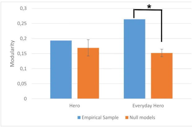
The modularity value of the Hero network (Q=.19) was not significantly higher than the corresponding modularity values of the null (random) models (p=0.19; mean=.17; standard deviation=0.027). In case of Everyday Hero, the modularity value of every (4999) independent null model was lower (p<.001; mean(random)=.15; standard deviation(random)=0.013) than the modularity value calculated for the social representation network (Q=.26). These results showed
33
that the Hero network was non-modular and the Everyday Hero network was modular (Figure 3.2).
Figure 3.2. The modularity values of the Hero (left) and Everyday Hero (right) networks comparing to the null models. The error bars refer to the standard deviation of the modularity value derived from the null models. The modularity value of the Hero network (Q=.19) was not significantly higher than the corresponding modularity values of the null models suggesting a cohesive representation. The modularity value of the Everyday Hero network (Q=.27) was significantly higher than the modularity values of the null models referring to multiple socio-cognitive categories.
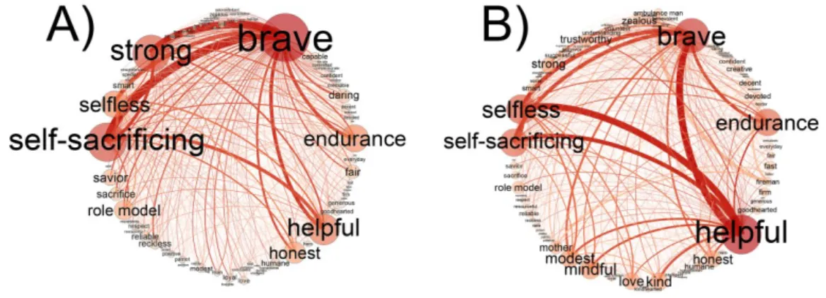
The visualization of the networks can be seen in Figure 3.3.
34
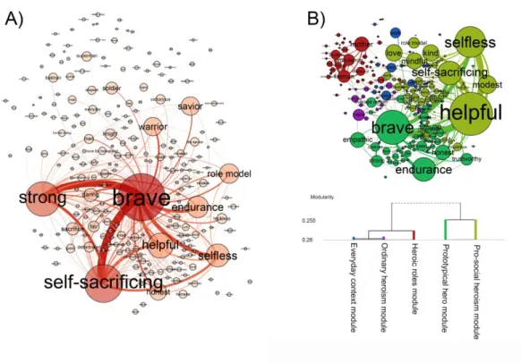
Figure 3.3. The social representations of Hero (A) and Everyday Hero (B). The association networks are visualized with the ForceAtlas 2 layout. The size of a node denotes the node strength and the thickness of an edge refers to the edge weight. The networks were thresholded (edges below the value of 1 were deleted) for a better visualization. In case of Everyday Hero, nodes with the same color belong to the same module. The hierarchy and descriptive labels of the modules are presented on the dendrogram.
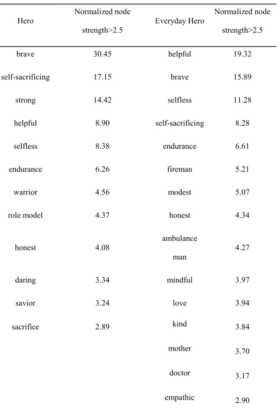
We identified the global hubs of the Hero and Everyday Hero networks (Table 3.1.). Hero is a network in which “brave” has an outstanding number of connections and it is followed by a couple of weaker global hubs. The global hubs of Hero are predominantly abstract values (“brave”, “self-sacrificing”, “strong”, “helpful”, “selfless”, “endurance”, “honest”, “daring” and
“sacrifice”). Among the global hubs of Hero, three concrete nodes appear: “warrior”, “role- model” and “savior”. Everyday Hero also has both abstract and concrete global hubs. The concrete global hubs (“fireman”, “ambulance man”, “mother” and “doctor”) are roles and occupations associated with heroism. The abstract global hubs (“helpful”, “brave”, “selfless”,
“self-sacrificing”, “endurance”, “modest”, “modest”, “honest”, “mindful”, “love”, “kind” and
“emphatic”) are associations expressing heroic values.
35
Hero Normalized node
strength>2.5
Everyday Hero Normalized node strength>2.5
brave 30.45 helpful 19.32
self-sacrificing 17.15 brave 15.89
strong 14.42 selfless 11.28
helpful 8.90 self-sacrificing 8.28
selfless 8.38 endurance 6.61
endurance 6.26 fireman 5.21
warrior 4.56 modest 5.07
role model 4.37 honest 4.34
honest 4.08
ambulance man
4.27
daring 3.34 mindful 3.97
savior 3.24 love 3.94
sacrifice 2.89 kind 3.84
mother 3.70
doctor 3.17
empathic 2.90
Table 3.1. Global hubs of the Hero and Everyday Hero networks. Normalized node strength > 2.5 refers to the global hubs of the association network.
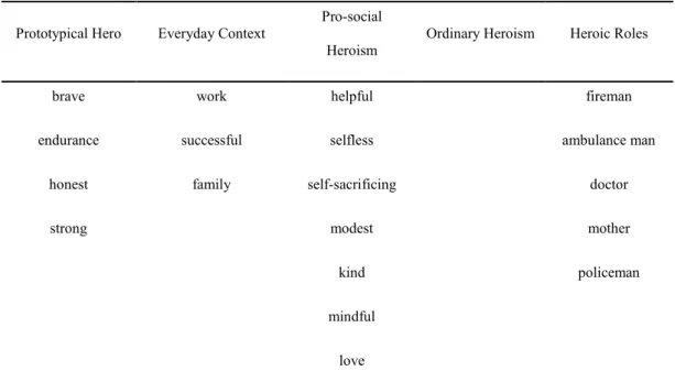
In case of Everyday Hero, we identified five modules. We labeled each of them based on their modular hubs resulting in the following: Prototypical Hero module, Everyday Context
36
module, Pro-social Heroism module, Ordinary Heroism module and Heroic Roles module (Table 3.2.). Prototypical Hero and Pro-social Heroism belong to a superordinate group while Everyday Context, Ordinary Heroism, and Heroic Roles form another group (see the
dendogram in Figure 3.3). Ordinary Heroism is a homogenous subnetwork and its nodes are relatively weakly tied. The only association that has node strength close to the threshold is
“mere”.
Prototypical Hero Everyday Context
Pro-social
Heroism Ordinary Heroism Heroic Roles
brave work helpful fireman
endurance successful selfless ambulance man
honest family self-sacrificing doctor
strong modest mother
kind policeman
mindful
love
Table 3.2. Modular hubs of Everyday Hero network. Normalized node strength > 2.5 refers to the modular hubs of the association network.
We calculated how many concrete social roles and contexts are present in the social
representation of Hero. We found that 38 out the 222 nodes (17.1%) were occupations (e.g., doctor, fireman, etc.), social roles (e.g., warrior, savior, etc.) or concrete characters (e.g., superheroes, historical figures, etc.).
3.3.1 Structural differences of the common associations
We gathered the common associations of the two social representations and created two networks from them representing either Hero or Everyday Hero (Figure 3.4). The number of
37
common associations was 85. The list of common associations is available in S4 File. A moderate correlation (r < .58, p < .001) was determined for the edge weights connecting the same nodes in the common association networks. In case of Hero, the majority of the edges are connected to “brave” with dominant links to “strong” and “self-sacrificing” (see in Figure 3.4/A). In case of Everyday Hero, the dominant edges are more balanced between “helpful”,
“selfless”, “self-sacrificing” and “brave” and even the less important edges seem to be more homogenously distributed (see in Figure 3.4/B). All modules of Everyday Hero were present among the common associations (the quotient of the number of participating nodes from a module and all nodes of the module expressed in percentage) as follows: Prototypical Hero module: 55%; Everyday Context module: 32%; Pro-social Heroism module: 40%, Ordinary Heroism module: 40%; Heroic Roles module: 26%. The global hubs of the original networks were among the nodes of the common association networks except for “warrior” in Hero and
“empathic” in Everyday Hero. Prototypical Hero module, Pro-social Heroism module and Ordinary Heroism module overlap to the highest degree with the social representation of Hero.
These modules contain abstract heroic values and characteristics. Everyday Context module and Heroic Roles module are present in lower proportion among common associations. They are more concrete in terms of content. They contain social roles, occupations and social contexts.
Figure 3.4. Common associations in the social representations of Hero (A) and Everyday Hero (B). The associations are arranged in a circular alphabetic order. The size of a node denotes the node strength and the thickness of an edge refers to the edge weight. The network was thresholded (edges below the value of 1 were deleted) for a better visualization.
38
3.4 D
ISCUSSIONThe psychological investigation of heroism is relatively new. At this stage, inductive methods can shed light on its main aspects. Therefore, we examined the social representations of Hero and Everyday Hero by constructing two networks from their free word associations. The results showed that the social representation of Hero is more centralized and it cannot be divided into smaller units. The network of Everyday Hero is divided into five units and the significance moves from abstract hero characteristics to concrete social roles and occupations exhibiting pro- social values. We also created networks from the common associations of Hero and Everyday Hero. The structures of these networks showed a moderate similarity and the connections are more balanced in case of Everyday Hero.
We showed that Abric’s [42], [65] theoretical framework about the central core vs. periphery associations is correspond to the scale-free organization of the association networks. Beyond the network interpretation of the classical Abric [65] model (central core of the social representation = the set of global hubs), we determined the modules and their modular hubs, which represent socio-cognitive patterns in the social representations based on Wachelke’s theoretical assumptions [66].
Several scholars suggested multiple categories for heroism [32], [35], [37]. Hence, we expected that Hero would have a modular structure that could be interpreted in accordance with prior categorizations. However, the Hero network is non-modular. Contrary to Hero, the social representation of Everyday Hero includes five modules: Pro-social Heroism, Prototypical Hero, Heroic Roles, Everyday Context and Ordinary Heroism (Figure 3.3). In the Hero network, a large proportion of the nodes express social roles, occupations or social contexts. However, they are not organized into modules. This means that the presence of similar elements does not guarantee that they will form coherent units in the structure of the social representation.
39
Everyday Hero has more concrete contents which are mainly present in Heroic Roles, Ordinary Heroism and Everyday Context modules. In case of both Hero and Everyday Hero, the abstract values and characteristics are in accordance with previous inductive studies [31]–[34]. Changing the topic form “hero” to “everyday hero” resulted in not only a different content but it created an entirely new network structure i.e., different global hubs (central cores), modular organization and more balanced connections of heroic contents. While heroism depicts doing something extraordinary in an abstract manner, everyday heroism implies just doing the right thing and it points out the ordinary roles, occupations and contexts in which the heroic values can be exhibited.
4 T HE MODULAR INVESTIGATION OF FREE WORD ASSOCIATION NETWORK CAN REVEAL POLARIZED OPINIONS
4.1 I
NTRODUCTIONIn the present study, we aim to use one socially prominent issue as a cue (refugee/migrant labelled as migrant) to capture opinions shared by a social group (Hungarians) [65], [67], [68]. As a measure of public opinions, the free association method can be viewed as a semi-structured alternative between traditional questionnaires producing highly structured data and web-mining algorithms collecting large quantities of unstructured data. Hence, the free association method can overcome the predefined scope of questionnaires [69] since respondents can express freely their opinion, yet, it has the advantage of representative samples and fast data processing as opposed to several web-mining methods [70]. Traditionally, free association analysis focuses on consensual meaning (i.e., most frequent words and rankings) regarding a social object [65], [67], [68] and they do not focus on the polarization of opinions [71]–[74].
Different prior word association methods were introduced to distinguish the stable and recurrent associations from peripheral ones. Szalay and Brendt [75] developed the Associative Group Analysis approach of free associations. In this method, the early associations in a