CHAPTER TEN
DILUTE SOLUTIONS OF NONELECTROLYTES.
COLLIGATIVE PROPERTIES
The material that follows has been separated from the preceding chapter primarily because a somewhat special emphasis is involved. A very important situation is that in which two phases are in equilibrium, one of which is a solution and the other of which is a pure phase of one of the components. The description is a general one of a system exhibiting a colligative property (from the Latin colligatus or collected together). The common feature of colligative properties is that, to a first approxi- mation, the observed behavior depends on the mole fraction composition of the solution and on the physical properties of the component which is present in both phases but not on the nature of the second component. The former will be defined as the solvent and the latter as the solute.
This common feature is an exactly observed one if the solution phase is ideal in its behavior. What is actually required is that the activity coefficient of the solvent be independent of the chemical nature of the solute; this condition will always be approached as xx-+\, since Raoult's law is the general limiting law for all solutions. Alternatively stated, it is usually desirable that the solution phase be dilute with respect to the solute. There is therefore considerable emphasis in this chapter on the behavior of dilute solutions.
The most important types of phase equilibria which give rise to colligative phenomena are given in Table 10-1. Other combinations are possible, of course, but are not encountered very often and are therefore ignored here.
One of the important applications of colligative phenomena is to the determination of the molecular weight of a solute present in dilute solution. There are a number of other methods for such a determination and these are reviewed in Section 10-7 so as to provide a general picture of this aspect of physical chemistry.
Colligative property measurements on nonideal solutions give the thermo- dynamic mole fraction or activity of the solvent and, indirectly, the activity and activity coefficient of the solute. This constitutes a second major application of colligative phenomena and is described in some detail in the Special Topics section.
Although appropriate to this chapter, chemical equilibria involving nonelectrolytes are more conveniently discussed in Chapter 12 along with equilibria involving electrolytes.
353
T A B L E 1 0 - 1 .
Phases in equilibrium Restriction or condition
N a m e of resulting colligative
property Liquid solution ^ vapor
Solid % liquid solution
Liquid solution % liquid solvent
Solute must be nonvolatile
Solid phase must consist of pure solvent Semipermeable membrane
prevents the solute from entering the pure solvent phase
Vapor pressure lowering Boiling point
elevation Freezing point
depression Osmotic pressure
10-1 Vapor Pressure Lowering
The general statement for the vapor pressure of the solvent component of a liquid solution is
Λ = β Λ ° [Eq. (9-71)]
or
4^ =
1-
<*i > O0"1)where AP1 is the vapor pressure lowering of the solvent, Ρλ° — P1. If the solute is nonvolatile, then Ρ is the total vapor pressure above the solution and ΔΡΧ is the total vapor pressure lowering Δ P.
If the solution is ideal, then Raoult's law, Eq. (9-4), holds, which means that ax = x1. Equation (10-1) becomes
(10-2)
still assuming the solute to be nonvolatile. Thus a measured behavior of the solvent has given the mole fraction of the solute, independent of the chemical nature of the latter. As will be illustrated later, if the weight composition of the solution is known, then the value of x2 can be used for calculation of the molecular weight of the solute.
10-2 Boiling Point Elevation
We can use the procedures of Section 9-6 to relate the change in normal boiling point of a solution to the solvent activity if the solute is nonvolatile. The situation is that since Ρ = 1 atm, ^ ( g ) = /xi°(g), and for phase equilibrium μχ(1) is therefore
10-2 BOILING POINT ELEVATION 355 equal to μ10(g). Thus
fh°(g) = fhff) = /*i°(0 + Win a, (10-3) [from the definition of ax, Eq. (9-72)].
Differentiation with respect to temperature gives
= -^°(/) + R In ax + RT , (10-4)
and on replacement of R In a1 by \μ^{έ) — ^ι°(/)]/Γ and following the procedure of Section 9-6,
dQn ad _ ΗΛΟ - # i ° ( g ) = ΔΗ$Λ
dT RT2 RT2 9 y }
where ΔΗ°Λ is the standard heat of vaporization of the pure solvent. Equation (10-5) may be integrated between limits, with ax = 1 at Τ = Γ £β 1, the normal boiling point of the pure solvent:
with 7b denoting the normal boiling point of a solution of solvent activity a1. We next consider the solution to be ideal. Equation (10-6) becomes
Again, a measurement of a property due to the solvent has yielded the mole fraction composition of the solution: x2 may, of course, be calculated from In χλ.
It was noted in the opening remarks that we obtain the condition of ideality in practice by using a dilute solution. Equation (10-7) undergoes considerable simplification under this condition. First, In x± may be expanded and only the first term of the series used, so that In xx ^ — (1 — xx) = — x2. For example, if x2 < 0.01, the error in the approximation is less than 1 %. With this substitution, and after rearrangement, Eq. (10-7) becomes
J r b = ΚΔΗ^ X*> (1°-8)
where Δ 7b is the normal boiling point elevation of the solution, 7b — ΤζΛ . The expansion of the In χλ term has already limited the maximum value of x2 to be tolerated, and no significant further error is introduced if 7\> is approximated by ΤζΛ in the numerator of Eq. (10-8). Also, we have
*2 = + = m + (1000/Λ/0 9 ( 1 0"9 ) where m is the molality of the solute and M1 is the molecular weight of the solvent.
The error due to neglecting m in the denominator of Eq. (10-9) is again not impor
tant. With these further approximations Eq. (10-8) becomes
where is called the boiling point elevation constant. depends only on properties of the pure solvent. The value for water is 0.514; further values are given in Table 10-2 in Section 10-4.
10-3 Freezing Point Depression
The equilibrium between a solid phase consisting of pure solvent and a liquid solution is treated as follows. The condition of equilibrium is that /χι°(^) = μλ{ϊ).
Then, by Eq. (9-72), we have
= Mi°(0 + RT In αλ. (10-11)
The rest is analogous to the preceding derivation. Differentiation with respect to temperature yields
-Sx°{s) = -Sx\l) + R In ax + RT , (10-12)
and, on replacement of R In ax by [μι%?) — /x!°(/)]/rand rearrangement, we have dQnad Ηλ\1) - Hx\s) = ΔΗ°ίΛ
dT RT2 RT* ' K }
Equation (10-13) is then integrated between limits, with ax = 1 at Tttl, the melting (or freezing) point of the pure solvent, to give
where Tt is the freezing point of the solution of solvent activity ax. Notice the parallel that is developing between the boiling point elevation and freezing point depression effects.
If the solution is ideal, Eq. (10-14) becomes
Again, the most valid application will be to dilute solutions, for which In x± may be approximated by — x2, so that
ΔΤ<=*%φ-χ2, (10-16)
and, by setting Tt = rf°t l and neglecting m in the denominator of Eq. (10-9), we obtain
Jr
' = [w^]- = ^ <
10-
17>
Kt is called the freezing point depression constant; its value depends only on properties of the solvent. F o r water, Kf = 1.86. Further values are given in Table
10-2.
10-4 SUMMARY OF THE FIRST THREE COLLIGATTVE PROPERTIES 357
10-4 Summary of the First Three Colligative Properties
The preceding two derivations were made on a somewhat formal thermodynamic basis and it is possible to give a physical explanation of all of the effects so far discussed. This is done in Fig. 10-1, which shows schematic vapor pressure plots for pure solid and pure liquid solvent and for a dilute solution of a nonvolatile solute. The vapor pressure lowering follows directly. The boiling point elevation is the difference between the two temperatures at which the Ρ = 1 atm line crosses the i V ( / ) and Λ(0 curves.
As noted in Section 8-4, at the melting point of a pure substance the solid and liquid vapor pressures must be the same. Therefore T?tl is the temperature of crossing of the Pi(s) and P^{1) curves. Since the solute is not present in the solid phase, the vapor pressure of the solid is not altered by the presence of solute, and Tt must therefore be the temperature of crossing of the a nd Λ(0 curves.
One objection to this last analysis is that it is not strictly necessary that the solute be nonvolatile in the freezing point depression effect. It is only necessary that it be insoluble in the solid solvent phase.
The boiling point elevation and freezing point depression effects are the more commonly used of the three, and some of the experimental aspects are as follows.
Figure 10-2 shows a Cottrell boiling point apparatus, the main feature of which is the tubular yoke around the bulb of the thermometer. The purpose is to bathe the bulb in boiling solution; were vapor simply allowed to condense onto the bulb, the temperature registered would tend to be that of the boiling point of the solvent, since the vapor consists of pure solvent.
Freezing point depressions may be obtained with very simple equipment, often consisting merely of a Dewar flask equipped with a Beckmann thermometer and a stirrer. The freezing point of the pure solvent is first determined, as, for example, by using a mixture of ice and water if the system is aqueous or in general by gradual cooling of the solution until freezing sets in. The experiment is repeated with the solution. Liquids tend to supercool, and it is necessary to be sure that enough finely divided solid solvent is present to ensure equilibrium.
F I G . 10-1. Explanation of boiling point elevation and freezing point depression effects in terms of vapor pressure changes. The solute is assumed to be nonvolatile.
100 Th
t, ° C
F I G . 10-2. Cottrell boiling point apparatus.
It is also essential to know the composition of the equilibrium solution that corresponds to the temperature measurement. This is not difficult in the case of boiling elevation; if the boiling solution is under reflux, its composition is essentially the same as that initially. In the freezing point depression experiment, however, there is apt to be appreciable freezing or melting before the final temperature reading, and a sample of the solution should be withdrawn for analysis at that point.
The vapor pressure lowering effect, while less frequently used, is actually quite important for very precise work. Rather than attempting direct vapor pressure measurements, however, one usually compares the unknown with a known solution by allowing the two solutions to come to vapor pressure equilibrium at a known temperature. For example, an open beaker of each solution might be placed in an otherwise empty desiccator, which is then thermostated. Solution A contains a known nonvolatile solute and solution Β contains the nonvolatile one being studied. The solvent vapor pressures above the two solutions will initially not be the same. Suppose that at first PltA is greater than P1 > B . Then solvent will distill from solution A to solution B, concentrating the former and diluting the latter. Eventually isopiestic equilibrium is reached, that is, P1A = PltB . The solutions must now have identical values for solvent activity ax. Analysis of solution A then determines the actual value of altA . Since the solutions are in equilibrium, altA = alfB . If solution Β is ideal or is dilute enough that Raoult's law has been reached as a limiting law, then altB = xltB .
10-5 OSMOTIC EQUILIBRIUM 359
T A B L E 10-2. Boiling Point Elevation and Freezing Point Depression Constants
Solvent >b( ° C ) t,(°Q
Ethyl ether 34.4 2.11
Chloroform 61.2 3.63 —
Ethanol 78.3 1.22 —
Benzene 80.2 2.53 5.6 5.12
Water 100.0 0.514 0.00 1.855
Acetic acid 118 3.07 17 3.90
Bromobenzene 155.8 6.20 — —
Naphthalene — — 80.2 6.8
Camphor — — 178 4 0
The isopiestic method has an advantage over the other two in being an isothermal one, so that corrections for changes in solvent properties with temperature are not needed. The isopiestic method is tedious, however, and is only used when very accurate results are wanted.
Representative values of and Kt are given in Table 10-2; some are quite large and such solvents are often used in qualitative molecular weight deter
minations because of the ease of measuring Δ Th or Δ Tt. It should be pointed out that both constants, but especially , depend on the ambient pressure. Thus Kh for benzene changes by 0.025 % per Torr difference between 760 Torr and the actual barometric pressure.
Example. T h e following illustrates the three effects. S u p p o s e that a n a q u e o u s solution o f a n organic c o m p o u n d is in isopiestic equilibrium with 0.1 m sucrose at 25°C. What is the vapor pressure of the solution if that of pure water is 23.76 Torr at 25°C? What would be the boiling point elevation and freezing point depression ? If the solution contains 2.50 wt % of the c o m pound, what is its molecular weight?
T o answer the first question, w e need the m o l e fraction of the sucrose solution: JC2 = 0.1/
[0.1 + (1000/18)] = 0.00180. T h e vapor pressure lowering is then (0.0018)(23.76) = 0.0428 Torr.
The solution of the c o m p o u n d must have the same value for ax as the sucrose solution and is dilute enough that we can use the dilute solution approximation; the molality of the two solutions is therefore also the same. The boiling point elevation is then (0.514)(0.1) = 0.0514°C, and the freezing point depression is (1.855)(0.1) = 0.1855°C.
W e have 25 g of c o m p o u n d per 975 g of water or 25.6 g per 1000 g of water. Since the solution is 0.1 m, the molecular weight must be 256.
10-5 Osmotic Equilibrium
An osmotic equilibrium is one between a solution and pure solvent, both liquid.
It is necessary to have a barrier between the liquids to separate them. The barrier must be impermeable to the solute, yet for equilibrium it must be permeable to the solvent. Such barriers or membranes (since they usually are thin) are called semipermeable membranes. The solvent activity is different in the two liquids, being lower in the solution than in the pure solvent; to bring the system to equi
librium, it is necessary to have the solution under mechanical pressure. The effect of such pressure on a pure liquid was shown in Section 8-5 to increase its vapor pressure or activity, and the same is true for a solution. The pressures involved
F I G . 1 0 - 3 . Schematic osmotic pressure apparatus.
can be considerable, and a semipermeable "membrane" usually must be either well supported or itself quite strong.
A schematic osmotic pressure apparatus is shown in Fig. 10-3. In the form pictured, solvent passes through the semipermeable membrane until sufficient hydrostatic head develops on the solution side for the activity of water in the solution to be equal to that of the pure solvent. Alternatively, the solution may be placed under sufficient mechanical pressure to just prevent net flow of solvent.
A simple demonstration of osmotic pressure is described in Fig. 10-4.
Osmotic equilibrium is independent of how the membrane acts so long as it is in fact permeable only to the solvent. The condition for equilibrium is that Pi(l) = μχ(1), where μλ(1) is the chemical potential of the solvent in the solution.
For a solution not under pressure,
fh(0 = /*i°(0 + RT In ax [Eq. (9-72)]
and the effect of pressure is, according to Eq. (8-22), to increase μχ{ϊ) by the integral of V1 dP:
)*i(0 = μι (I) + RT In ax + Γ Vx dP. (10-18) At equilibrium the free energy of the solvent must be the same on both sides of
the diaphragm, or
μι°(1) = μι(0 = μι°(0 + RT In αλ + f V1 dP
JPi°
or
-RT In ax = (10-19)
The required mechanical pressure Π to produce equilibrium is known as the osmotic pressure. Ordinarily Π is large compared to Px° and the change in Vx with pressure
10-5 OSMOTIC EQUILIBRIUM 361
F I G . 10-4. Filter paper moistened with water and acting as a "leaky" membrane between chloroform (in the tube) and ether. Chloroform is quite insoluble in water and the wet filter paper acts as a barrier to its passage. Ether, however, is sufficiently soluble in water to diffuse through the "membrane."
can be neglected, so Eq. (10-19) simplifies to
-RT\nax = TIV1. (10-20)
If the solution is ideal, then ax = xx and
-RTlnx
1=nV
1.
(10-21) If the solution has approached ideality by also being dilute, then In xx may beapproximated by —x2, as before. At the same level of approximation x2 ~ n2\nx, and so Eq. (10-21) takes the very simple form
RT^ =
nV
1°.
In the case of a dilute solution nxVx is essentially the volume of the solution, so
Πν = n2RT or Π = CRT. (10-22)
The interesting final result is that in dilute solution osmotic pressure obeys the ideal gas law. The final approximation is unnecessarily severe, and a very useful dilute solution form is one in which C is the number of moles of solute per unit volume of solvent, rather than per unit volume of solution.
Example. T h e e x a m p l e o f the preceding section m a y be extended t o the calculation o f the osmotic pressure of the solutions. The osmotic pressure Π must be the same for the sucrose solution and that of the unknown c o m p o u n d at 25°C since they are in isopiestic equilibrium.
Then C = 0.1 m o l e liter"1 of solvent and Π = (0.1)(0.0821)(298) = 2.45 atm. N o t e h o w large the osmotic pressure is compared to the other colligative effects.
T A B L E 10-3. Osmotic Pressure of Aqueous Sucrose at 0°Ca
Concentration (grams per liter
of solution) (Λ,/ΛΟ Χ 104
Osmotic pressure (atm) Concentration
(grams per liter
of solution) (Λ,/ΛΟ Χ 104 Observed Equation (10-22) Modified Eq. (10-21)*
2.02 1.064 0.134 0.132 0.133
10.0 5.294 0.66 0.655 0.661
45.0 24.22 2.97 2.947 3.056
300 193.6 26.8 19.65 26.99
750 737.2 134.7 49.14 154.5
"Source: E. A . Moelwyn-Hughes, "Physical Chemistry," p. 803. Pergamon, Oxford, 1961.
6 See text.
Some data due to Berkeley and Hartley in 1906 on the osmotic pressure of sucrose solutions are given in Table 10-3. The simple formula (10-22) fails badly by about 1 m sucrose concentration, and even the more exact form, Eq. (10-21), is inadequate;
it would predict an osmotic pressure of 92 atm for the most concentrated solution, instead of the observed 134.7 atm. We have confidence in the thermodynamics, and evidently the solution must not be ideal, as assumed in writing Eq. (10-21).
It turns out, however, that the quite reasonable agreement shown by the last column of Table 10-3 results if one supposes that each sucrose molecule binds six molecules of water. The actual number of moles of solvent present is thus reduced by six per mole of sucrose present, and x2 is correspondingly increased.
This example is cited to illustrate one way in which a formal nonideality may be accounted for.
10-6 Activities and Activity Coefficients for Dilute Solutions
The use of activities and activity coefficients for solutions was discussed in Section 9-5. It will be recalled that activity a was defined as the effective mole fraction such as to keep the form of Raoult's law:
Pi = α,Ρ* [Eq. (9-71)].
The activity coefficient γ was defined as the factor whereby a differs from x, Oi = ViXi [Eq. (9-73)],
so that the chemical potential for the ith species is
/**(/) = μΜ) + RT In a{ [Eq. (9-72)].
Since Raoult's law is approached by all solutions as xt 1, it follows that in this limit at —• Xi and γ{ —• 1.
This convention is fine for solutions of two liquids, whose compositions can range from pure component 1 to pure component 2. It is, however, very awkward for dilute solutions, and an alternative set of definitions has become customary
10-6 ACTIVITIES AND ACTIVITY COEFFICIENTS FOR DILUTE SOLUTIONS 363 for the solute. That for the solvent remains the same. Since Henry's law is the limiting law for the solute, we now define an activity a' such that Henry's law is obeyed,
P2 = a2'k2. (10-23)
The corresponding activity coefficient y2 is given by
a2' = y2' * 2 · (10-24)
These conventions are to be applied only to the solute, and Eqs. (10-23) and (10-24) have been written on this basis. Since Henry's law is approached as x2 0, then a2 —>• x2 and y2 —> 1 at this limit.
In the case of aqueous solutions, it is customary to express the concentration of solute as molality m rather than as x2. Henry's law may still be used as a limiting law since by Eq. (10-9), m and x2 become proportional as x2 —• 0, and in this limit
Activity is now defined by and activity coefficient as
P2 = mkm . (10-25)
P2 = amkm (10-26)
dm = Vrrjn. (10-27) As x2, and hence m9 approaches zero, am-+m and ym 1. Finally, x2 or m becomes
proportional to C, the concentration in moles per liter of solution, as the concen
tration approaches zero. Henry's law becomes P2 = Ckc, and a concentration- based activity ac may be defined as
p2 = ackc . (10-28)
The corresponding activity coefficient yc is
ac = ycC (10-29)
Again, as x2, and hence C, approaches zero, a c ^ C and yc - * 1.
The subject is discussed in more detail in the Special Topics section, but it turns out that the effect of using the Henry's law conventions is to change the reference or standard state, and hence the value of /xt°(/) of Eq. (9-72). All equations involving only changes in activity remain the same, but in using the Gibbs-Duhem equation, as in Section 9-5, the first integration limit is x2 = 0 rather than x2 = 1 since it is now the former condition for which γ = 1 and hence In γ = 0. Alternatively, y2 differs from y2 by a constant factor. However, mole fraction, molality, and concentration cease to be proportional in concentrated solutions, and as a con
sequence the three types of activity coefficient differ. The general relationship among them is
y2 = ymO + O.OOlmMi) = yc- - , (10-30)
where M2 is the solute molecular weight, ρ is the density of the solution, and p° is the density of the pure solvent.
A. Sedimentation Velocity
It is possible to estimate the size of a molecule by the speed with which it moves through a solution under the influence of some force. One such force is that due to gravity. A particle of mass m2 experiences a downward pull of m2g, opposed in solution by the buoyancy of the solvent. In effect, the particle displaces volume m2\p2, corresponding to a mass of solvent equal to (m2/p2) px, where p2 and ρλ are the densities of the particle and of the solvent, respectively. The net force due to gravity is then
\ P2 ι
where v2 is the partial specific volume of the particle.
The particle will fall through the solution if p2 > p1, but as it accelerates a viscous drag develops which is proportional to the velocity, or equal to fv, where υ is the velocity and / is called the friction coefficient. A limiting or terminal velocity is reached when the force due to gravity and that of the viscous drag have become equal, or when
ν = Τ . (10-32) f
In liquids of ordinary viscosity, this terminal velocity is reached very quickly, and the experimental observation is that the particle immediately assumes a constant speed of fall.
The friction coefficient depends in a complicated way on the shape of the particle and on the viscosity of the solvent. However, if the particle is spherical, a simple formula due to Stokes applies:
/ = 6πψ, (10-33) where η is the viscosity of the medium and r is the radius of the particle. The velocity
of fall is then
(10-34)
10-7 Other Methods of Molecular Weight Determination
One of the important uses of colligative property measurements is to obtain the molecular weight of a solute. This is particularly true for new substances being characterized for the first time, including biological species such as proteins or nucleic acids. Polymer chemistry is also a highly developed field, and a central piece of information is again the molecular weight of a particular preparation.
In this case there will usually be a mixture of various molecular weights and one seeks to determine the average value (as will be discussed later).
There are several other means whereby either the size or the molecular weight of a solute may be determined and it seems appropriate to include these in the present chapter.
10-7 OTHER METHODS OF MOLECULAR WEIGHT DETERMINATION 365 The particle is to be a solute molecule, although perhaps a large one such as a protein, and its rate of fall due to gravity will be extremely small—so small, in fact, that, as will be seen, it is quickly nullified by back-diffusion. It is therefore ordinarily necessary to increase the sedimentation force by using a centrifuge. Acceleration due to gravity is replaced by ω2χ9 where ω is the angular velocity (in radians per second) and χ is the distance from the center of rotation. Equation (10-32) becomes
dx _ m2oj2x(l - v2Pl) n n ^
dt f ' U UO J J
or
* = ^ ( 1 - Ϋ Λ ) , S
= ^T< <
10-
36)
where s is called the sedimentation coefficient and is characteristic of a given solute and solvent.
Example. F o r a laboratory centrifuge, χ might b e a b o u t 10 c m a n d the speed o f rotation 50 rps. T h e force ω2χ is then ( 2 π )2( 5 0 )2( 1 0 ) or a b o u t 1 x 10* c m s e c "2 or 10*g. A protein molecule o f molecular weight 100,000, or particle weight 1.66 x 1 0 ~1 9g , a n d o f specific v o l u m e 0.80 c m8 g "1 w o u l d then sediment with a rate o f (1.66 x 1 0 "1 9) ( 1 x 1 0e) ( l - 0 . 8 ) / / , or a b o u t 3.3 x 1 0 "1 4/ / , in c m s e c "1. If the particle is spherical, w e h a v e
frrr3 = (1.66 χ 10-l f l)(0.8) ~ 1.3 χ 10"1 9,
from which r is f o u n d t o be 3.2 x 1 0 "7 c m . T h e viscosity o f water is a b o u t 0.89 c P a n d , by Stokes' law, / = 6π(0.0089)(3.14 x 1 0 "7) = 5.4 x 1 0 "8c m s e c "2. T h e velocity o f sedimenta
tion o f the protein molecules w o u l d then be (3.3 x 1 0 "1 4) / ( 5 . 4 x 1 0 "8) , or a b o u t 6.1 x 1 0 "7 c m s e c " \ a rather small number.
The calculation illustrates the difficulty in carrying out sedimentation experiments with ordinary centrifuges. A Swede, The Svedberg, pioneered in the 1920s the development of very high-speed centrifuges or ultracentrifuges. Forces as high as 300,000g have been obtained. The sedimentation rate would be 300 times larger than in the preceding example, or about 2 χ 1 0 "4 cm s e c '1, an easily measurable rate. Centrifuges of this type may be air-suspended and air-driven. More elegantly, the rotor can be suspended by a magnetic field and driven by induction. In the latter version, the rotor chamber is evacuated so that friction is virtually absent.
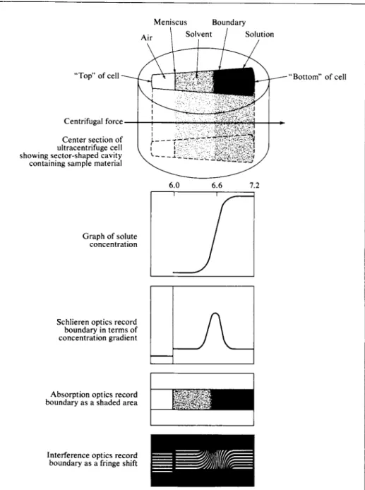
The cell containing the solution is placed in the rotor and can be viewed through windows. Stroboscopic pictures of the boundary formed by sedimenting material can be obtained with the use of synchronous lighting, and the sedimentation velocity thus determined. The molecular weight may then be found, essentially by reversal of the preceding calculation. One contemporary type of ultracentrifuge is described in Fig. 10-5.
B. Diffusion
A second type of kinetic approach which yields information about molecular size is that of diffusion studies. The coefficient of diffusion is defined phenomeno- logically by Fick's law,
J = - @ ? [Eq-(2-65)],
FIG. 1 0- 5 . The analytical ultracentrifuge.
(a) The system. The rotor (l)is driven by means of a flexible drive shaft that makes it so nearly self-balancing that loads need only be balanced to 0.5 g.
Speeds up to 60,000 rpm and 370,000 times gravity acceleration are routine.
The rotor chamber may be cooled by the refrigerator unit (2) and is evacu- ated by mechanical (3) and diffusion (4) pumps. Light from the source (5) passes through the sample cells and out the light pipe (6) to a scanner or a cam- era. A set of slits allows light to pass only as the cell comes into position.
(Courtesy Spinco Division, Beckman Instruments, Palo Alto, California.)
(b) The optics. (Courtesy Spinco Divi- sion, Beckman Instruments, Palo Alto, California.)
10-7 OTHER METHODS OF MOLECULAR WEIGHT DETERMINATION 367
Meniscus Boundary Solution
"Top" of cell
Centrifugal force Center section of ultracentrifuge cell showing sector-shaped cavity containing sample material
Graph of solute concentration
Schlieren optics record boundary in terms of concentration gradient
Absorption optics record boundary as a shaded area
Interference optics record boundary as a fringe shift
Bottom" of cell
FIG. 10-5. (c) Illustration of various optical systems for recording the boundary region formed between solution and supernatant liquid in moving boundary ultracentrifugation. {From H. C.
Ehrmantraut and P. D. Quattrone in "Ultracentrifugal Analysis in Theory and Experiment"
(J. W. Williams, ed.), Academic Press, New York, 1963.]
where Of is the diffusion coefficient and / is the molecular flux along the con- centration gradient, in molecules per square centimeter per second. Diffusion occurs because molecules in solution drift around under random kinetic motion and more move from a high-concentration region than from a low-concentration region. It is purely as a statistical effect that net flow occurs down a concentration gradient.
The flow may be treated as a net bias in the otherwise random motion, whereby molecules appear to exhibit a net velocity ν in the direction of the concentration gradient. The flux / can therefore be represented as
/ = nv. (10-37) We now invoke a force to produce the velocity v, namely the gradient of chemical
potential —άμζ\άχ or — kTd(\n a)/dx. The velocity is then
ν = - kTdQna)ldx , (10-38)
Γ
and combination of Eqs. (2-65), (10-37), and (10-38) gives _ kTn d(\n d)\dx _ φ dn
f ~ dx or
kT </(ln a)
f rf(lnn) (10-39)
It is convenient to use the convention of ac , so that d(\n ac) = d(\n C) + d(\n yc) (see Section 10-6) and since d(\n n) = d(\n C) (n and C are proportional), Eq.
(10-39) reduces to
In the case of dilute nonelectrolyte solutions y c will approach unity, and Eq. (10-40) is often used in the limiting form
kT
9 = £±-. (10-41)
f
Equation (10-40) was obtained by Einstein in 1905 (see Section 16-CN-l for a historical sketch).
The formalism of the chemical potential gradient as a driving force in diffusion is just that—a formalism. It is a very convenient one, however, and more elaborate analyses based on the statistics of individual molecular motions give the same result.
As in the case of sedimentation rates, one may consider the diffusing molecule to be spherical and apply Stokes' law. The diffusion coefficient becomes
kT
9 = -τ—- . (10-42) It is thus possible to obtain a molecular radius from diffusion data. Small molecules
have diffusion coefficients in water of about 1 0- 5 c m2 sec"1 at room temperature and hence corresponding r values of about (1.37 χ 10-1 6)(298)/(67r)(0.01)(10-5) = 2.2 χ 1 0- 8 cm, or of a few angstroms. The values obtained agree fairly well with estimates from van der Waals constants or from crystallographic determinations of molecular sizes. In general, even though the exact form of Stokes' law may not be correct, Eq. (10-42) is often obeyed to the extent that 2η is a constant; the observation is known as WalderCs rule.
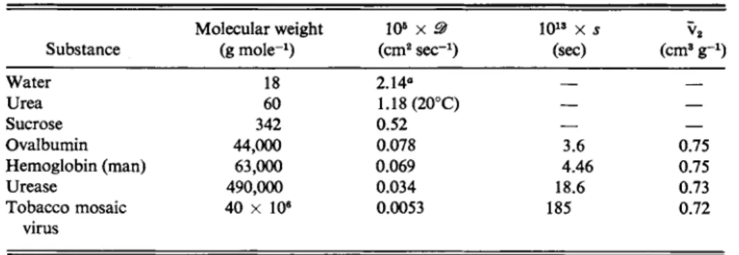
10-7 OTHER METHODS OF MOLECULAR WEIGHT DETERMINATION 369 It is difficult to measure diffusion coefficients smaller than about 1 0- 7 cm2 s e c- 1, so that the method begins to fail for molecular weights above 106 (see Table 10-4).
In summary, diffusion coefficients provide a measure of the hydrodynamic radius of a molecule and thereby information about its molecular weight.
C. Sedimentation Equilibrium
We may now combine the two preceding subsections to treat sedimentation equilibrium. The dynamic picture is that a molecule under the influence of gravity or a centrifugal field will move in the direction of the force, so that a concentration gradient develops. Eventually the back-diffusion rate becomes equal to the sedi
mentation rate. That is, ν in Eq. (10-32) and ν in Eq. (10-38) may be equated to give
m2g(l - v2 P l) = k T ^ ± . (10-43) The friction coefficient is the same for both processes, and therefore cancels out.
Rearrangement gives
^ ) = M ( 1 _ v 2 P l ) , (10-44) or, in dilute solution
^ W " - ^
(10"
45)Except for the necessary buoyancy correction, Eq. (10-45) is the same as the barometric equation (1-34); if integrated, with dx = —dh9 it yields
m2g'hy
where, to bring out the comparison, g has been replaced by the effective force due to gravity g\ where g' = g(l - v ^ ) .
Alternatively, Eq. (10-41) may be used to eliminate / in Eq. (10-36), to give
* = ^ ( 1 - ν Λ ) (10-46)
or
M2 = — . (10-47)
0 ( 1 - v ^ )
Thus if both the sedimentation and diffusion coefficients are known, the molecular weight may be determined without any assumptions as to the size or shape of the molecule.
To return to sedimentation equilibrium, we see that if g in Eq. (10-45) is replaced by ω2χ and the equation is integrated between the limits Cx at x1 and C2 at x2, the result is
IRTlniCJCJ / 1 Λ / Ι 0,
TABLE 10-4. Diffusion and Sedimentation Coefficients (in Water at 25° C)
Substance
Molecular weight (g m o l e- 1)
ΙΟ5 χ 9 ( c m2 s e c- 1)
ΙΟ1 3 χ s (sec)
v2
( c m8 g_ 1) Water
Urea Sucrose Ovalbumin Hemoglobin (man) Urease
Tobacco mosaic
44,000 63,000 490,000 40 χ 10e
18 60
342 0.52
0.078 0.069 0.034 0.0053 2 . 1 4e
1.18 (20°C)
3.6 4.46 18.6 185
0.75 0.75 0.73 0.72 virus
aT h i s is a self-diffusion coefficient obtained by isotopic labeling.
Sedimentation equilibrium studies using ultracentrifuges have provided a great deal of information about the molecular weights of large molecules such as proteins, other biological substances, and polymers. The method is tedious in that consid
erable time is required to attain equilibrium. A modern variant involves the use of a gradient in the density of the medium. The effect is greatly to accentuate the equilibrium concentration distribution, and molecular weights as low as about 300 can be determined by this means.
Example. T h e numerical example o f Section 10-7A m a y b e extended to Eq. (10-48). W e take ω2 to be 1 χ 1 05, the molecular weight to be 100,000, and v2 t o be 0.80, and a s s u m e that x2 and xx are 4 and 3 c m , respectively. T h e n
Some values for diffusion and sedimentation coefficients are given in Table 10-4.
D. Light Scattering
The subject of light scattering by small particles is a complicated one and will be treated here only in a superficial way. In terms of the electromagnetic theory of light, incident radiation induces an oscillating dipole in a molecule or particle, which in turn reradiates. The intensity of scattered light therefore depends on the polarizability a; it is also a function of angle, being a maximum in the direction of the incident beam.
The detailed analysis was begun by Lord Rayleigh in 1900, extended by G. Mie around 1908, and further extended by P. Debye in 1947. The intensity of unpolarized light scattered by a single molecule is given by
where, as illustrated in Fig. 10-6,10 is the incident light intensity per square centi
meter, ι is the intensity per square centimeter observed at scattering angle Θ, oc is the polarizability of the scattering molecule, λ is the wavelength of light, and r is
C , ( 1 0 0 , 0 0 0 ) 0 x 1 05) ( 42 - 32)(1 - 0.80)
d (2)(8.3 x 10⁷)(298) ~ 0.28.
16TT4(X2(1 + cos2 Θ)
A4r2 (10-49)
10-7 OTHER METHODS OF MOLECULAR WEIGHT DETERMINATION 371 y
1 + c o s2 θ X
F I G . 10-6. Intensity envelope for scattered light. The envelope is a figure of revolution about the axis defined by the incident light.
the distance from the scattering particle. Some of the important features of Eq. (10-49) are as follows:
(1) The intensity depends inversely on λ4 and is therefore much stronger for blue than for red light. Small-molecule scattering in our atmosphere brings blue light to us from the sky and yellows or reddens direct sunlight, especially at sunset when the distance traveled through the atmosphere is larger than at other times.
(2) The minimum scattering occurs at 90°. The qualitative reason is that the induced dipoles are oriented perpendicularly to the incident light and reradiate most strongly in the same direction.
(3) The dependence on the polarizability has been accounted for.
In the case of a dilute solution or suspension of scattering molecules or particles, a useful modification of Eq. (10-49) is the following. Assuming additivity of molar refractions, Eq. (3-15) may be manipulated to give n2 — n02 = 4wN0<*clM. Here, η is the index of refraction of the solution and n0 that of the solvent; c is the con
centration in grams per cubic centimeter of scattering molecules of polarizability a and molecular weight M. For a dilute solution, η2 — n02 = (n + n0)(n — n0) ~ 2n0c dn/dc and we obtain
Since the number of particles per cubic centimeter is cNJM, the total scattering is ι 4π2Μ2(\ + cos2 Θ) n02(dn/dc)2
N02X*r2 (10-50)
4ττ2(1 + cos2 Θ) n2(dn\dcj N0X*r2
|2 Mc. (10-51)
We next integrate the scattered intensity over all angles, to obtain the total proportion of light removed from the incident beam. The removal of light by scattering produces the same mathematical law as for the absorption of light
(see Section 3-2),
/ = i0e-**, (10-52)
where / is the intensity of unscattered light and τ is called the turbidity. The proportion of light that is scattered is then (/0 — I)jl0 and for small amounts of scattering this is equal to τ for a 1-cm path length. The result of the integration over all angles and the introduction of τ is
T = * Α Γ \ Α — - Mc = HMc, (10-53)
where
and therefore
_ 327T3n02(dn/dc)2 n f t ^
* = (10-55) Actual practice is somewhat more complicated. Solution nonidealities cause
deviation from Eq. (10-55), so the quantity He/τ is usually plotted against c and extrapolated to zero concentration. Further, the reduction in light intensity of the direct beam is rather small, so it is difficult to measure /0 — / accurately. A better procedure is to determine i at some definite angle, most commonly 90°, and use Eq. (10-49) to relate the scattering intensity at that angle to the total scattering corresponding to r. A further complication is that if the particles are comparable in size to the wavelength of the light used, there will be interference effects arising from light scattered from different parts of the same particle. If this is a problem, then i/I0 is measured at various angles and the calculated Η values are extrapolated to θ = 0, where such interference vanishes. This is done for each of several concentrations and the set of extrapolated points lies on a line which can in turn be extrapolated to zero concentration. A clever way of making the two extrapola
tions (to zero c and to zero 0) is due to Zimm (1948).
Light scattering can be used for any size molecule; one may, for example, observe scattering from a pure liquid due just to the fluctuations in density that occur, and the scattering by the atmosphere has already been mentioned. Equation (10-53) states, however, that for a given concentration in grams per cubic centimeter the larger the molecular weight, the greater the scattering. The method is then most sensitive for macromolecules and has been widely used in the study of biological and synthetic polymers.
£. Types of Molecular Weight Averages
It is particularly true for polymer solutions (discussed further in Chapter 20) that a preparation will consist of a range of molecular weights. A molecular weight determination by one of the methods of this chapter will give an average value but, it turns out, not always the same average one as that given by some other method.
There are two principal ways in which one may average the molecular weight of a collection of solute molecules. The first is the intuitive one of simply dividing
COMMENTARY AND NOTES, SECTION 1 373 the total weight by the total number of particles. This is known as the number average molecular weight Mn and is defined formally as follows:
M n = n1M1 + n i M + - = = ^
« 1 ~ h «2 "Γ jLi ni i
Thus a sample consisting of equal numbers of molecules of molecular weight 100, 1000, and 10,000 g m o l e- 1 would have a number average molecular weight of
M n =
KiQQ) + Kiooo) + έ(ΐο,οοο)
= 3 7 0 0In this case each molecular weight is weighted by the number of particles involved. An alternative weighting is by the weight of particles of a given molecular weight (or essentially by their size):
M = wxMx + w2M2 + - = 2i WiMj = Σ ί niM? (10-57) wx + w2 + - Σι Wi W t o t
Mw is known as the weight average molecular weight. Referring to the example just given, since there are equal numbers of each kind of molecule,
( 1 0 0 ) 2 + (1000)* +(ΙΟ,ΟΟΟ)2 100 + 1000 + 10,000
In this case, as in general, the weight average molecular weight is greater than the number average molecular weight. The ratio of the two gives a measure of the total spread of molecular weights in the sample.
The colligative property measurements essentially count the number of particles and one obtains the molecular weight by dividing the weight of material present by this number. The result is therefore a number average molecular weight.
Sedimentation experiments weight each particle according to its mass and there
for give a weight average molecular weight. The same is true of light scattering measurements.
COMMENTARY AND NOTES 10-CN-l Colligative Properties and Deviations from Ideality
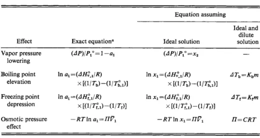
The equations for the four colligative properties are summarized in Table 10-5.
They group into three categories: (1) the forms that are strictly valid (except for the assumed constancy of heats of vaporization and freezing, and of activity coeffi
cients with temperature), (2) those that assume an ideal solution, and (3) those that assume an ideal and dilute solution. A number of systems have been studied very precisely, and there seems to be no question that Raoult's law is a valid limiting law, at least for solutions not involving molecules grossly different in size. Also,
TABLE 10-5. Colligative Property Equations
Equation assuming
Ideal and dilute
Effect Exact equation0 Ideal solution solution
Vapor pressure (ΔΡ)ΙΡ^ = \ -αι
(ΔΡ)ΙΡ
χ*=χ
% —lowering
Boiling point In ai=(AHyJR) In Xl=(AHy°JR) ATh=Khm
elevation
xKi/r^-o/O]
Freezing point In a^iAHlJR) In x^iAHlJR) ATt=Ktm
depression
χ[(ΐ/τ7.ι)-(ΐ/τν)] xta/O-d/r,)]
Osmotic pressure -RTln α1=ΠΫ1 -RT\n χ1=ΠΫ1 n=CRT
effect
a The last three of these equations are not fully exact. Assumptions such as constancy of heat of vaporization or heat o f freezing have been made in integration over Δ Th or Δ Tt. In the case o f o s m o t i c pressure, other assumptions, noted in the text, have been m a d e . These are n o t drastic assumptions, and in this text the equations given are regarded as thermodynamically exact.
heats of fusion from Kt values agree well with those from direct calorimetric determinations.
Although these affirmations are important, it is also true that deviations from the simple behavior are common. We discount immediately cases in which the dilute solution forms have been misused in that the conditions for the mathematical approximations have not been met. There remain several explanations. One is that the solute is either associated or dissociated to some extent, so that its apparent molecular weight differs from its formula weight. Remember that the colligative property effects are determined by x2, the mole fraction of solute. This mole fraction is determined by the actual species present. As one example, the molecular weight of benzoic acid is just the formula weight of 122.1 in acetone solution, but in benzene, the apparent molecular weight is 242. That is, the colligative property measurement reports half as many solute molecules as expected from the amount weighed out in making u p the solution. The explanation is that benzoic
acid is largely dimerized in benzene solution.
Alternatively, if the freezing point depression is determined for an aqueous sodium chloride solution the result gives an apparent molecular weight that is about half the formula weight. In this case we have a strong electrolyte which has dissociated into two ions, each of which acts as a solute species with respect to a colligative property. The Dutchman van't Hoff, who contributed much to the physical chemistry of the osmotic pressure effect, defined a factor / as
Πν = in2RT, (10-58)
where the simple meaning of i is that it gives the average number of moles of particles produced per formula weight of solute. Thus / would be \ for benzoic acid in benzene and 2 for aqueous sodium chloride. The approach, while over
simplified, emphasizes the point that the colligative property measurement gives an average molecular weight. One may thus use the measurement to calculate the degree of association or, for a weak electrolyte, the degree of dissociation. In the
COMMENTARY AND NOTES, SECTION 2 375 case of polymer solutions, where a wide range of molecular weight species is present, the average molecular weight that results is known as a number average (see Section 10-7E).
Another source of deviation from ideal behavior is illustrated by the data of Table 10-3. It appears, from this as well as from other evidence, that sucrose tightly binds about six molecules of water. The situation is essentially one of com
pound formation between solute and solvent, and the effect on a colligative property measurement is that the effective value of xx is reduced while that of x2 is increased.
A fair measure of the departure from ideal behavior of electrolyte solutions can be accounted for if each ion, especially the positive ion, is assumed to bind a certain number of water molecules.
The resemblance of the ideal osmotic pressure equation, Eq. (10-22), to the ideal gas law was noted in Section 10-5. The resemblance extends further. Just as non- ideal gases can be represented by a virial equation (Eq. 1-37), so can the osmotic pressure of a nonideal solution,
R=l+B(T)c--,
(10-59)where c is concentration in grams per cubic centimeter.
Finally, departures from ideality may always be treated in a nonspecific way by calculating ax from use of the exact equation. The solute activity, a2, and activity coefficient, y2 >m a v then be obtained by the methods of Section 10-ST-l.
10-CN-2 Relationship between Freezing Point Depression and Solubility
In dealing with colligative property effects, we have consistently applied the term solvent to that component which is present in both phases. Thus in the case of a freezing point depression Eq. (10-15) may be written
In xA =
and applies to the equilibrium system
pure solid A ^ ideal solution of A and B, (10-60)
where A denotes solvent, by the preceding convention, and Β denotes solute. The laboratory appearance of such an equilibrium mixture is simply one of a suspension of a solid in a solution, and the system could just as well be described as a saturated solution of solid A in solvent B, with excess solid A present.
When viewed according to this alternative perspective, Eq. (10-15) gives the solubility of component A, now thought of as the solute, in solvent component B.
Now Tf is no longer described as a freezing point, but just as Γ, the temperature at which the solubility is measured. As an example, the freezing point of a 0.25 mole fraction solution of, say, ethanol, in acetic acid should be approximately 0°C (assuming ideal behavior). The calculation is made, from Eq. (10-15), with acetic acid as the solvent. Alternatively, the same value denotes the solubility of solid