CHAPTER ONE IDEAL AND NONIDEAL GASES

CHAPTER ONE

IDEAL AND NONIDEAL GASES

1-1 Introduction

Physical chemistry comprises the quantitative and theoretical study of the properties of the elements in their various states of combination. The definition is a sweeping one—it includes the behavior and the structure of individual molecules as well as all the various kinds of intermolecular interactions. At one time physical chemistry was considered to be a part of physics; and physics, yet earlier, lay within the formal discipline of natural philosophy. This historical relationship is reflected in the name "doctor of philosophy" for the highest degree in science.

The name should not be considered as a purely archaic one, however; the chemist and other scientists are philosophers in that they inquire into the underlying causes of natural behavior.

Science, or the second philosophy as it is sometimes called, has progressed far indeed; moreover, its development shows no signs of slackening. For example, we need not go back very far in time—say thirty years—to observe that many topics in this book were once either unknown or at the research frontier. During this thirty year period an avalanche of facts has been compressed by the physical chemist into tables of standard data and into far-reaching empirical relationships, and the great theories of physics and chemistry have been made more precise and more capable of treating complex situations. New phenomena—the natural world is still full of surprises—have been discovered, measured, and then fitted within a theoretical framework. The same processes are going on today—the student thirty years from now will no doubt be confronted with much material not to be found in present texts.

The textbook of physical chemistry has never been easy to assimilate (or to write !)

—there is so much to cover and there are so many important things to emphasize.

The major empirical laws must be described and the great theories of molecular dynamics, statistical thermodynamics, and wave mechanics must be treated in sufficient detail to provide both a real appreciation and a foundation for more advanced work. Furthermore, throughout the book the tone of the writing should be quantitative, not descriptive; the student should experience the scientific method at work.

The material that follows has been written in as plain and direct a way as this 1

1-2 Equations of State

A system at equilibrium may be described by the macroscopic properties of volume v, pressure P, and temperature t. (Temperature is defined for the moment by means of some arbitrarily chosen thermometer, and we neglect the need to specify what magnetic, electric, or gravitational fields are present.) That is, all other properties of the system are determined if these variables are specified. The equation of state of a system is just the functional relationship

ν = mf(P, t\ (1-1) where m is the mass present and f(P, t) is some function of pressure and

temperature. If V denotes the molar volume, an alternative form of Eq. (1-1) is

V=f(P,t). (1-2) As a matter of convenience, an equation of state usually is written for a pure

writer knows. Much attention has been given to its organization. The student should read the preface carefully; it describes the philosophy of the book, its structure, and various practical aspects of its use. One point should be mentioned here. It is assumed that the student has taken a modern course in introductory college chemistry and that he is reasonably familiar with the gas laws, simple thermodynamics and the concept of chemical equilibrium, and the elements of chemical kinetics. Such background material is generally reviewed briefly early in each chapter. The student is also assumed to be comfortable with the qualitative language of wave mechanics and chemical bonding, although no detailed background in these subjects is required.

Both cgs (centimeter-gram-second) and SI (Systèm e International e o r meter - kilogram-second-ampere) unit s wil l b e used . Th e forme r syste m i s th e traditiona l one i n chemistry . However , th e bette r feature s o f th e newe r S I syste m ar e gainin g use i n th e Unite d States . A s discusse d mor e full y i n Chapte r 3 (Sectio n 3-CN-l) , the difference s becom e substantia l mainl y i n th e are a o f electrica l units . Som e conversion table s ar e give n o n th e insid e o f th e fron t cover .

We procee d no w t o th e topi c o f thi s chapter . I n keepin g wit h th e abov e assump - tions, w e wil l no t belabo r th e idea l ga s la w o r it s simpl e applications . W e d o show , in Sectio n 1-3 , ho w th e la w i s obtained , bu t wit h th e purpos e o f demonstratin g how i t i s use d t o defin e a temperatur e scale . Th e procedur e provide s a beautifu l illustration o f th e scientifi c method ; a quantit y suc h a s temperatur e i s a ver y subtle on e i n it s ultimat e "meaning, " ye t w e ar e abl e t o defin e i t exactl y an d unambiguously.

The barometri c equatio n receive s a goo d dea l o f attentio n i n thi s chapter . Thi s is partl y becaus e o f it s ow n usefulnes s an d partl y becaus e th e equatio n serve s t o introduce a principl e o f far-reachin g importance—th e Boltzman n principle . The res t o f th e chapte r deal s wit h th e behavio r o f nonidea l gase s an d wit h critica l phenomena. Som e previou s experienc e wit h thi s subjec t i s assume d an d th e materia l is therefor e covere d rathe r briefly . Th e mai n emphasi s i s o n th e va n de r Waal s equation becaus e i t i s s o widel y use d fo r th e qualitativ e treatmen t o f rea l gases . A glimps e o f th e mor e rigorous , moder n approac h i s give n i n th e Specia l Topic s section.

1-3 THE IDEAL GAS; THE ABSOLUTE TEMPERATURE SCALE 3

1-3 Development of the Concept of an Ideal Gas; the Absolute Temperature Scale

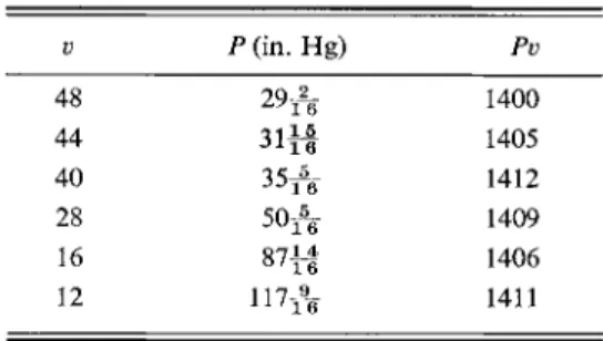
The first reported reasonably quantitative data on the behavior of gases are those of Robert Boyle (1662). Some of his results on "the spring of air" are given in Table 1-1 ; they show that for a given temperature, the Pv product is essentially constant. Much later, in 1787, Charles added the observation that this constant

TABLE 1-1. "The Spring of Air" (Boyle, 1662)a

ν Ρ (in. Hg) Pv

48 A yl 6 1400

44 ^{11 1A} J 11 6 1405

40 35-^- 1412

28 50-A ¹⁴⁰⁹

16 8 7 f | 1406

12 117 A ¹⁴¹¹

aN o t e Fig. 1-1.

chemical substance; if a mixture is involved, then composition is added as a variable.

Note that P, t, V, and density ρ = m/v are intensive quantities. That is, their value does not depend on the amount of material present. Total volume ν and mass m are extensive quantities. The latter gives the amount of the system and the former is proportional to m as indicated by Eq. (1-1). It is customarily assumed that an equation of state can always be written in a form involving only intensive quantities as in Eq. (1-2). This expectation is more a result of experience than a fundamental requirement of nature. We know, for example, that if a sufficiently small portion of matter is sampled, then its intensive properties will depend on its mass. In fact, one way of taking this aspect into account is by adding a term for the surface energy of the system. Such a term is ordinarily negligible and will not be considered specifically until Chapter 8.

To resume the original line of discussion, an equation of state describes a range of equilibrium conditions for a substance. That is, we require Eq. (1-2) to be obeyed over an appreciable range of the variables and that its validity be inde­

pendent of past history. Suppose, for example, that some initial set of values (P, t) determines a molar volume Vx, and that Ρ and / are then varied arbitrarily.

It should be true that if they are returned to the original values, then Κ returns to Vx. An equation such as Eq. (1-2) is aphenomenological one; it summarizes empirical observation and involves only variables that are themselves experimentally defined.

Such relationships are often called laws or rules. In contrast, theories or hypotheses draw on some postulated model or set of assumptions and may not be and in fact usually are not entirely correct. A phenomenological relationship, however, merely reflects some aspect of the behavior of nature, and must therefore be correct (within the limits of the experimental error of the measurement).

Robert Boyle: 1627-1691 As the son of the Earl of Cork, he was born to wealth and nobility. While residing at Oxford, he discovered 'Boyle's law," methyl alco­

hol, and phosphoric acid, and noted the darkening of silver salts by light. In "The Sceptical Chymist," he at­

tacked the alchemical no­

tion of the elements, giving an essentially modern defi­

nition. A founder of the Royal Society. (From H. M.

Smith, "Torchbearers of Chemistry," Academic Press, New York, 1949.)

Two of Boyle's Experiments

FIG. 1-1. On the left : A demonstration that a paddle wheel of feathers fell rapid­

ly in a vacuum, and without turning. Boyle was seeing if air had some "subtle " com­

ponent that could not be re­

moved. On the right: How Boyle obtained the data of Table 1-1. (From "Robert Boyle's Experiments in Pneumatics" J. B. Conant, ed., Harvard Univ. Press, 1950.)

Mercury column increased by pouring mercury

in at Τ ^

Shorter leg with scale

Initial level of mercury

1-3 THE IDEAL GAS; THE ABSOLUTE TEMPERATURE SCALE 5

was a function of temperature. At this point the equation of state for all gases was observed to be

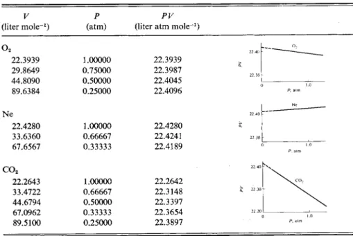
Pv=f{t). (1-3) Very accurate contemporary measurements add some important refinements.

A selection of such results is given in Table 1-2, and we now see that not only does the PV product depend on pressure at constant temperature, but it does so in different ways for different gases. The data can be fitted to the equation

PV = A(t) + b(t)P + c(t)P2 + - · · (1-4) where t in parentheses is a reminder that the coefficients A, b, c, etc., are tempera­

ture dependent. The important observation is that while b, c9 and so forth depend also on the nature of the gas, the constant A does not. As Ρ -> 0, Eq. (1-4) becomes

PV = A(t)9 (1-5) where, at 0°C, A(t) = 22.4140 for V in liter m o l e-1 and Ρ in atmospheres. Note

that Eq. (1-5) is a limiting law, that is, it gives the behavior of real gases in the limit of zero pressure.

If now the value of A(t) is studied as a function of temperature, one finds the approximate behavior to be (as did Gay-Lussac around 1805)

A = j + kt. (1-6) The values of j and k depend on the thermometer used; moreover, the temperature

dependence of A is not exactly linear. Specifically, the results obtained using a mercury thermometer are not quite the same as those obtained using an alcohol thermometer. It is both arbitrary and inconvenient to have a temperature scale tied

TABLE 1-2. Isothermal P-V Data for Various Gases at 0°C

(liter mole- 1^{) (atm) Ρ} (liter atm mole^PV - 1) o2

22.3939 29.8649 44.8090 89.6384

1.00000 0.75000 0.50000 0.25000

22.3939 22.3987 22.4045 22.4096 Ne

22.4280 33.6360 67.6567

1.00000 0.66667 0.33333

22.4280 22.4241 22.4189 c o2

22.2643 33.4722 44.6794 67.0962 89.5100

1.00000 0.66667 0.50000 0.33333 0.25000

22.2642 22.3148 22.3397 22.3654 22.3897

TABLE 1-3.

Units0 R

liter atmosphere mole "1 Κ -1 0.082057 cubic centimeter atmosphere mole "1 Κ "1 82.057

joule mole"1 Κ "1 8.3143

erg mole"1 Κ "1 8.3143 χ 107

calorie mole"1 Κ "1 1.987

° Degree absolute is denoted by K.

to the way some specific substance, such as mercury or alcohol, expands with temperature. The constant A9 however, is a universal one, valid for all gases and we therefore use Eq. (1-6) as the defining equation for temperature.

The limiting gas law thermometer, or, as it is usually called, the ideal gas thermom­

eter is commonly based on a centigrade scale; the specific defining statements are as follows:

(1) t = 0 at the melting point of ice, at which temperature A = 22.4140;

(2) t = 100 at the normal (1 atm) boiling point of water, at which temperature , 4 = 30.6197;

(3) intervening t values are defined by A — j + kt.

On combining these conditions, we have

j = 22.4140, k = 0.082057

(using liter m o l e-1 and atmosphere units). Equation (1-6) then becomes

A = 22.4140 + 0.082057i = 0.082057(273.15 + t), (1-7) where t is now the familiar temperature in degrees Centigrade (or Celsius).

The next step is obvious. Clearly Eq. (1-7) takes on a yet simpler and more rational form if a new temperature scale is adopted such that Τ = 273.15 + t°C.

We then have

A = 0.082057Γ, (1-8) or, inserting the definition of A into Eq. (1-5), we obtain

lim PV = RT. (1-9)

p->o

Τ is,called the absolute temperature and R is the gas constant, whose numerical value depends on the choice of units. Some useful sets of units and consequent R values are given in Table 1-3.

The procedure for obtaining Eq. (1-9) has been described in some detail not only because of the importance of the equation, but also because the procedure itself provides a good example of the scientific method. We have taken the pheno­

menological observation of Eq. (1-5), noticed the approximate validity of Eq.

(1-6), and then defined our temperature scale so as to make Eq. (1-9) exact. In effect, the procedure provides an operational, that is, an unambiguous experimental,

1-4 THE IDEAL GAS LAW AND RELATED EQUATIONS 7

definition of temperature. At no point has it been in the least necessary to under­

stand or to explain why gases should behave this way or what the fundamental meaning of temperature is.

To summarize, Eq. (1-9) is an equation obeyed (we assume) by all gases in the limit of zero pressure. As Boyle and Charles observed, it is also an equation of state which is approximately obeyed by many gases over a considerable range of temperature and pressure.

At this point it is convenient to introduce the concept of a hypothetical gas which obeys the equation

PV = RT (1-10) under all conditions. Such a gas we call an ideal gas. It is important to keep in mind

the distinction between Eq. (1-9) as an exact limiting law for all gases and Eq.

(1-10) as the equation for an ideal gas or as an approximate equation for gases generally. This type of distinction occurs fairly often in physical chemistry, such as, for example, in the treatment of solutions.

1-4 The Ideal Gas Law and Related Equations

Equation (1-10) can be put in various alternative forms, such as

Pv = nRT (n = number of moles); (1-11) Pv = — RT (M = molecular weight); (1-12)

PM = PRT (p = density). (1-13)

Equation (1-13) tells us, for example, that the molecular weight of any gas can be obtained approximately if its pressure and density are known at a given tempera­

ture. Furthermore, since the ideal gas law is a limiting law, the limiting value of P/p as pressure approaches zero must give the exact molecular weight of the gas.

In effect, by writing Eq. (1-4) in the form

P_Pv_RT β_Ρ , 7 ^ ! • ... Π-14)

p ~ m ~ M M M ' U 1 4J

one notes that the intercept of Pv/m (or P/p) plotted against Ρ must give RTjM for any gas. Such a plot is illustrated schematically in Fig. 1-2.

Example. The density of a certain hydrocarbon gas at 25°C is 12.20 g liter"1 at Ρ = 10 atm and 5.90 g liter"1 for Ρ = 5 atm. Find the molecular weight of the gas and its probable formula.

At 10 atm, P/p is 10/12.20 = 0.8197, and at 5 atm, it is 5/5.90 = 0.8475. Linear extrapolation to zero pressure gives P/P = 0.8753. Hence M = RT/(P/P) = (0.082057)(298.15)/(0.8753) = 27.95 g m o l e- 1. The probable formula is C2H4 .

Example. Convert the data above to SI units and rework the problem.

The SI unit of force is the newton, Ν ; this force gives an acceleration of 1 m sec"2 ^{to 1 kg.}

The SI unit of pressure is the pascal, Pa; 1 Pa is 1 Ν per m2^{. Thus}

1 atm = (0.760mHg)(13.5981 g c m -3) ( 1 0 "3 kg g - ^ l O6 c m3m "3) (9.80665 m s e c "2) = 1.01325 χ 105 Pa or Ν m~2.

Also,

1 g liter"1 = 1 kg m~3.

The problem now reads that the density is 12.20 kg m "3 at Ρ = 1.01325 x 10e Pa and is

5.90 kg m '3 at Ρ == 5.06625 x 105 Pa. The respective P/p values are 83,053 and 85,870 Pa m3 k g- 1, and the value extrapolated to zero pressure is 88,690 Pa m3 kg"1. The molecular weight is thus

M = (8.31433)(298.15)/(88690) = 0.02795 kg mole"1.

Note that in the SI system, molecular weights are a thousandfold smaller in numerical value than in the cgs system. This is because the unit of mass is the kilogram, while Avogadro's number remains the same.

FIG. 1-2. Variation of Pjp with Ρ for a hypothetical nonideal gas.

It is generally useful to have an accepted standard condition of state for a sub­

stance. Often this is 25°C and 1 atm pressure. In the case of gases, an additional, frequently used condition is that of 0°C and 1 atm pressure. This state will be referred to as the STP state (standard temperature and pressure).

1-5 Mixtures of Ideal Gases; Partial Pressures

So long as the discussion about gases deals with a single chemical species it is immaterial whether volume is put on a per mole or a per unit mass basis. If the amount of gas, expressed in either way, is doubled at constant temperature and pressure, the volume must also double. Suppose, however, that a container holds 1 g of hydrogen at STP, and 1 g of oxygen is added. The STP volume of the mixture will not be doubled; it would be, however, if 16 g of oxygen were added. (This last statement is strictly true only if the condition is the limiting one of zero pressure rather than 1 atm.)

We are involved at this point with another observation, embodied in the state­

ment known as Avogadro's hypothesis, which says that equal volumes of gases at the same pressure and temperature contain equal numbers of moles. Again this is really a limiting law statement, exact only in the limit of zero pressure, but approxi­

mately correct for real gases. In effect, the constant A of Eq. (1-4) is a universal constant only if V is volume per mole, and not, for example, per gram of gas. A more general form is thus

Pv = nA + nbP + ncP2 + · (1-15)

1-5 MIXTURES OF IDEAL GASES; PARTIAL PRESSURES 9

Since A is independent of the nature of the gas, η is simply the total number of moles of gas, irrespective of whether there is a mixture of species present. The corresponding ideal gas law is given by Eq. (1-11).

We now define the partial pressure of the ith species in a mixture of gases by the equation

PiV = n.RT. (1-16) Dividing Eq. (1-16) by Eq. (1-11) gives

li = Hi.

Ρ η or

Pi = XtP, (1-17) where x{ denotes the mole fraction of the ith species. Since the sum of all mole

fractions must by definition equal unity, it further follows that

Σ Pi = Λ (1-18) that is, the total pressure of a mixture of ideal gases is given by the sum of the partial

pressures of the various species present. This is a statement of Daltorts law.

A useful quantity which can now be defined is the average molecular weight of a gas, given by

Mav = ^ - , (1-19)

where m and η are respectively the total mass and number of moles present.

Further, we have

Mav =

Σρ. = Σψ±

.

It also follows, on combining Eqs. (1-13) and (1-18), that

PMav = pRT. (1-21) Thus the procedure illustrated by Fig. 1-2 will, for a mixture of gases, give the

average molecular weight.

A complication may now arise. In order to determine the exact average molecular weight of a gas mixture, it is necessary to extrapolate P/p to the limit of zero pressure, yet it can happen that the composition of the mixture is itself dependent on the pressure. Thus, gaseous N204 will actually consist of a mixture of N 02 and N204 in amounts given by the equilibrium constant for the process N204 = 2 Ν Ό2 :

Jf, = ^ L . (1-22)

^ N204

The proportion of N 02 present will increase as the total pressure decreases, so that Afav now varies with pressure. In effect, one now knows the species and hence their molecular weight and KP is the unknown. Equation (1-22) for KP is exact only for ideal gases, however, and the following procedure is necessary. One first determines Mav for a series of total pressures using Eq. (1-21). Each determination provides a value for KP , assuming ideal gas behavior, and these values are then

plotted against pressure. The true KP is given by the intercept at zero pressure.

See Problem 1-17.

1-6 Partial Volumes; Amagat's Law

The partial volume v{ of a component of a gaseous mixture is defined as the volume that com­

ponent would occupy were it by itself at the pressure and temperature of the mixture:

Since Σ n{ = n, it follows that and, further, that

riiRT

»< = - Ί Γ - . (1-23)

Σ^ = ν (1-24) Vi = x&. (1-25) Equation (1-24) is a statement of Amagat's law of partial volumes, and although its derivation

assumes ideal gas behavior, the equation is often more closely obeyed by real gases than is its counterpart involving partial pressures, Eq. (1-17).

1-7 The Barometric Equation

It was mentioned in Section 1-2 in discussing equations of state that initially we were neglecting to include as variables any magnetic, electric, or gravitational fields present. Ordinarily all three are present in any laboratory, but the first two are so small that they occasion only a negligible variation in intensive properties from one part of the system to another. The earth's gravitational field is large enough, however, that it cannot always safely be neglected. In the case of liquids the variation of hydrostatic pressure with depth can be quite significant. The same is true for gases if a long column of gas is involved, as in dealing with the atmosphere.

Not only is the gravitational field occasionally important, but the derivation of its effect that follows leads to an important new type of equation.

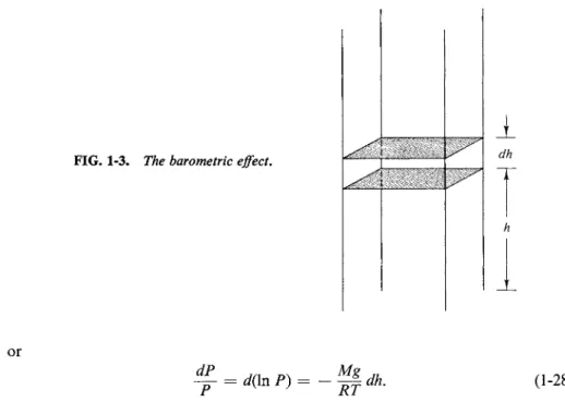
Consider a column of fluid of unit cross section as illustrated in Fig. 1-3. The pressure, or force per unit area, at level h must be just the total weight of the column above that level. The change in pressure dP between h and h + dh is then just the weight of fluid contained in the unit cross section in the column between the two levels:

dP= -pgdh, (1-26) where g is acceleration due to gravity. Equation (1-26) is general. If the fluid is a

liquid which is assumed to be incompressible, then ρ is independent of h and integration gives

P2 ~ Λ = -pg ΔΚ (1-27)

which is just a statement of the variation of hydrostatic pressure with height.

If, however, the fluid is taken to be an ideal gas, then use of Eq. (1-13) or (1-21) gives

dP = - g dh

1-7 THE BAROMETRIC EQUATION 11

FIG. 1-3. The barometric effect.

ι dh

or

dP

~ = d(\nP) (1-28)

[It is common to write rf(ln x) for dx/x or —diXjx) for Λ / χ2, and so on, as an anti­

cipation of integration.]

Equation (1-28) cannot be integrated unless something is known about how M, g, and Γ vary with h; one simple case is that in which these quantities are taken to be constant. The result, known as the barometric equation, is then

ln ^{Pn Mgh}

or

ρ __ ρ p-Mgh/RT

Example. As an application of Eq. (1-29) consider a column of atmosphere of Mav = 29 g m o l e- 1, Τ = 298 K, g = 980 cm sec"2^{, and P}0 = 1 atm at h = 0. The exponential term must be dimensionless, so R must now be in ergs K_1 m o l e-1 and h in centimeters. One then finds

* -

[mr^mmu -

-

"

·

Thus if h = 1 km, or 105 cm,

ph = e-O.ii48 _ ο 8 9 2>

Note that in the SI system, Mav = 0.029 kg m o l e- 1, g = 9.8 m sec"2, Λ is in meters, and R should be in joules K "1 m o l e- 1.

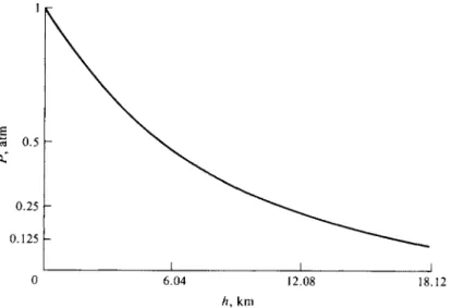
It is worth taking a moment to discuss some of the mathematical aspects of an exponential equation such as Eq. (1-30). In the example here a plot of Ρ versus h appears as shown in Fig. 1-4.

Note that at h = 6.04 km, Ph^IP0 = 1/2 or Ρ = 0.5 atm. The "half-height" or h1/2 (the height for the pressure to decrease by a factor of one-half) is independent of the actual value of P0. Thus, starting at 6.04 km, the pressure will decrease by half again in another 6.04 km, and so will be 0.25 at Λ = 12.1 km, and so on, as illustrated in the figure.

Equation (1-30) is of the general form

y - y0e-«* (1-31)

and the value of χ for y/y0 = 1/2, or the "half value" of χ, x1 / 2, is related to k as (1-29)

(1-30)

3 0.5

0.25

0.125 h

0 6.04 12.08 J_

h, km

18.12

FIG. 1-4. Decrease of barometric pressure with altitude for air at 298 K.

follows:

or

if JO 2 '

kx1/2 =

then In -kxll

(1-32) -In ^ = 0.6932.

Thus, in the example just given h1/2 = 0.6932/0.1148 = 6.04 km.

A further point is as follows. In view of the previously discussed laws for mixtures of ideal gases, Eq. (1-30) applies separately to each component of a mixture.

Thus each component of the earth's atmosphere has its own barometric distri­

bution, with the consequence that the pressures and hence concentrations of the lighter gases decrease less rapidly with altitude than do those of the heavier ones.

As a result the proportion of, for example, helium in the atmosphere increases with altitude.

Equation (1-30) may be expressed in yet a different way, and one which is very instructive. Under the assumed condition of constant temperature it follows from the ideal gas law that concentration C is proportional to pressure:

Ρ RT' Hence

Ch = C0e~M9h/RT = C0e-m9h^kT,

(1-33) (1-34) where m is now the mass per molecule and k is the gas constant per molecule, known as the Boltzmann constant. The quantity mgh is just the potential energy of a molecule at height h in the gravitational field, and Eq. (1-34) is a special case of the more general equation

ρ = (constant)e~e/f c r, (1-35) where ρ is the probability, here measured in terms of the concentration or pressure, of a molecule having an energy e. Equation (1-35) is a statement of the Boltzmann

1-8 DEVIATIONS FROM IDEALITY-CRITICAL BEHAVIOR 13 principle and is of central importance in dealing with probability distributions, as

in gas kinetic theory and in statistical thermodynamics.

1-8 Deviations from Ideality—Critical Behavior

The equation of state of an actual gas is given in one form by Eq. (1-4), PV = A(T) + b(T)P + c(T)P2 + ,

where b(T), c(T), and so on are not only functions of temperature, but also are characteristic of each particular gas. A form that is more useful for theoretical purposes is the following:

PV = A{T)[ B(T) , C{T) or

RT V K2

(1-36)

(1-37) This type of equation is known as a virial equation, and B(T) and C(T) are called the second and third virial coefficients, respectively. This form is more useful than Eq. (1-4) because molar volume is a measure of the average distance between molecules and an expansion in terms of V is thus an expansion in terms of inter- molecular distance. The virial coefficients can then in turn be estimated by means of various theories for intermolecular forces of attraction and repulsion.

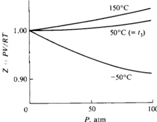
The left-hand term of Eq. (1-37), PV/RT, is called the compressibility factor Ζ and its deviation from unity is a measure of the deviation of gas from ideal behavior.

Such deviations are small at room temperature for cryoscopic gases, that is, low- boiling gases such as argon and nitrogen, until quite high pressures are reached, as illustrated in Fig. 1-5, but can become quite large for relatively higher-boiling ones, such as carbon dioxide. Figure 1-6 shows that for nitrogen at tz = 50°C (curve 2), the plot of the compressibility factor Ζ against Ρ increases steadily with increasing pressure, but at a lower temperature, it first decreases. At one

A, II Ν

1.0

0.8

^ H ^ 0 ° C ^ N2^{, 100°C}

-

^ \ c o2,1 0 0° C

50 P, atm

100

150°C 1.00

0.90

FIG. 1-5. Variation of compressibility factor FIG. 1-6. Variation of compressibility factor with pressure. with temperature and pressure for nitrogen.

particular temperature, the plot of Ζ versus Ρ approaches the Ζ == 1 line asymptotically as Ρ approaches zero. This is known as the Boyle temperature. The analytical condition is

The partial differential sign, d, and the subscript, T, mean that the derivative of Ζ is taken with respect to Ρ with the temperature kept constant. A gas at its Boyle temperature behaves ideally over an exceptionally large range of pressure essentially because of a compensation of intermolecular forces of attraction and repulsion.

The gas of a substance which can exist in both the gas and liquid states at a given temperature is often distinguished from gases generally by being called a vapor. Clearly, as a vapor is compressed at constant temperature, condensation will begin to occur when the pressure of the vapor has reached the vapor pressure of the liquid. The experiment might be visualized as involving a piston and cylinder immersed in a thermostat bath; the enclosed space contains a certain amount of the substance, initially as vapor, and the piston is steadily pushed into the cylinder.

The arrangement is illustrated in Fig. 1-7. At the point of condensation, reduction in volume ceases to be accompanied by a rise in pressure; more and more vapor simply condenses to liquid at constant pressure P°. Eventually all the vapor is condensed, and the piston now rests against liquid phase; liquids are generally not very compressible, and now great pressure is needed to reduce the volume further.

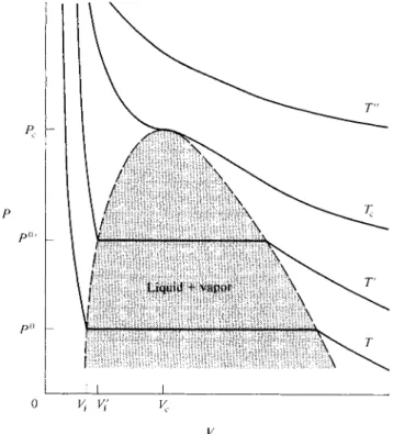
The plot of Ρ versus F corresponding to this experiment is shown in Fig. 1-8, where P° denotes the vapor pressure of the liquid and V\ its molar volume. The plots

FIG. 1-7.

1-8 DEVIATIONS FROM IDEALITY-CRITICAL BEHAVIOR 15

o vi v;

ν

FIG. 1-8. P-Visotherms for a real vapor.

are for constant temperature, or isothermal, processes and are therefore called isotherms.

As further illustrated in Fig. 1-8, at some higher temperature the isotherm will lie above the previous one, and the horizontal portion representing condensation will be shorter. This is because, on the one hand, P°f is larger than P°, so the molar volume of the vapor at the condensation point is smaller, and on the other hand, the liquid expands somewhat with temperature, so V{ is greater than Vx. One can thus expect, and in fact does observe, that at some sufficiently high temperature the horizontal portion just vanishes. This temperature is called the critical temperature Tc , and the isotherm for Tc is also shown schematically in Fig. 1-8. The broken line in the figure gives the locus of the end points of the condensation lines, and hence encloses the region in which liquid and vapor phases coexist.

There is not only a critical temperature, but also a critical point, which is the vestigial point left by the condensation line as it just vanishes; alterna­

tively, the critical point is the maximum of the broken line of the figure. This point then defines a critical pressure Pc and a critical volume Vc as well as Tc . The critical temperature can also be considered as the temperature above which we speak of a gas rather than of a vapor. Compression of a gas (that is, in this context, a gaseous substance above its critical temperature) results not in conden­

sation, but only in a steady increase in pressure, as illustrated by the curve labeled T" in Fig. 1-8.

Figure 1-8 also illustrates the difficulty of displaying a function of three variables on a two-dimensional plot. A true graph of V = f(P, T) requires a three-dimen-

sional plot, such as is represented in Fig. 1-9. On the other hand, while such a three-dimensional plot can thus be visualized, it is difficult to work with; hence the use of isothermal cross sections. It should be recognized, however, that cross sections can be taken in other ways. Thus the lighter lines in Fig. 1-9 correspond to the profiles of cross sections at constant temperature, or isotherms, and the broken lines to cross sections at constant volume, or isosteres {isometrics). Isobars, not shown, are cross sections at constant pressure. In general at sufficiently high temperatures and especially at sufficiently large volumes the curves for any sub­

stance will approach those for an ideal gas. In this limiting case one then has isotherms given by Ρ = (RT)(^ or hyperbolas,

(

(

At the other extreme, that of low temperatures and especially of small volumes, one has the liquid phase. The isotherms are then given by the coefficient of com­

pressibility of the liquid, β, defined as

' - - 7 ( • & • ) , < ' -3» Values of β for liquids are small, about 10~5 a t m- 1. Thus for small changes in

1-9 THE VAN DER WAALS EQUATION 17

volume the slope of the P-V isotherm for a liquid will be approximately — (l/Κβ);

for water at 20°C it is about 1.2 χ 106 atm liter- 1. Thus the curves in this region of Fig. 1-8 are nearly vertical lines. The isobars are given by the coefficient of thermal expansion oc defined as

Values of a are likewise small, about 10" 4 K "1 and the slope of the V-T isobar for a liquid will thus be Va for small changes in V. For water Va is about 8.0 χ 1 0 "6 liter K "1. Consequently isobars corresponding to the liquid phase appear as nearly horizontal lines.

The preceding digression was intended to help fix characteristic general features of the typical P-V-Τ relationship for a real substance, insofar as vapor and liquid phases are involved. At the moment, however, we are primarily interested in the vapor and gas regions and for these there is an important observation known as the principle of corresponding states. The intermolecular forces of attraction and repul­

sion which determine deviations from ideality also determine the conditions for condensation and, in particular, the values of Tc, Pc , and Vc . It is therefore perhaps not surprising that if the equation of state for a gas or vapor is written in the form

the function / turns out to be nearly independent of the nature of the substance.

The quantities P/Pc, V/Vc, and T/Te are known as the reduced variables and are denoted by Pr , VT , and TT , the reduced pressure, reduced volume, and reduced temperature, respectively.

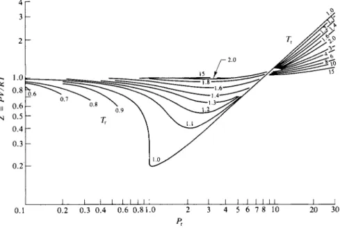
This statement about Eq. (1-41) is essentially a statement of the principle of corresponding states. Alternatively, the principle affirms that all gases at a given Pr and TT have the same VT . A corollary is that gases or vapors in corresponding states have the same value for Z, the compressibility factor. Figure 1-10 may be used to obtain a fairly good value for the compressibility factor and hence for V if Ρ and Τ are known, for any substance whose critical constants are also known.

The critical constants for a selection of substances are given in Table 1-4.

Example. Suppose that we wish to find the molar volume of ammonia gas at 212°C and 224 atm pressure. Then PT ^{and T}T are 224/112 = 2.0 and 485/405 = 1.2. From Fig. 1-10, point A, the value of Ζ for Pr = 2 and Tr = 1.2 is 0.57. The molar volume of the ammonia is then V = 0.5ΊRT/P = (0.57)(0.0821) (485)/(224) or V = 0.101 liter.

The relative success of the principle of corresponding states, as illustrated in the use of the chart of Fig. 1-10, suggests that it should be possible to find a not too complicated analytical expression for the function V = f(P, T). In fact quite a number of such functions have been proposed, some of which are given in the Commentary and Notes section at the end of the chapter. Such functions, being analytical, are in many ways more convenient than a graph such as Fig. 1-10; they (1-40)

(1-41)

1-9 Semiempirical Equations of

State. The van der Waals Equation

4 Γ

0.1 0.2 0.3 0.4 0.6 0.81.0 2 3 4 5 6 7 8 10 20 30

FIG. 1-10. Hougen- Watson chart for the calculation of pressure, volume, and temperature relations at high pressure. {From O. A. Hougen and Κ. M. Watson, "ChemicalProcess Principles "

Part II. Copyright 1959, Wiley, New York. Used with permission of John Wiley & Sons, Inc.)

TABLE 1-4. Critical Constants and Related Physical Properties'1

Melting Boiling

point point To

Substance (K) (K) (K) (atm) (cm3 mole- 1)

He < 1 4.6 5.2 2.25 61.55

Ne 24.5 27.3 44.75 26.86 44.30

H2 14.1 20.7 33.2 12.8 69.68

o2 ^{54.8 90.2 154.28} 49.713 74.42

N2 63.3 77.4 125.97 33.49 90.03

Cl2 172.2 238.6 417.1 76.1 123.4

CO 74 81.7 134.4 34.6 90.03

NO 109.6 121.4 177.1 64 57.25

c o2 ^216.6b 194.7 304.16 72.83 94.23

H20 273.2 373.2 647.3 218.5 55.44

N H3 ^{195.5 239.8 405.5 112.2} 72.02

CC14 ^{250.2 349.7 556.25 44.98 275.8}

CH4 90.7 109.2 190.25 45.6 98.77

C2H2 191.4 189.2 308.6 61.65 112.9

C2^H4 104.1 169.5 282.8 50.55 126.1

CH3OH 175.3 338.2 513.1 78.50 117.7

C2H5OH 155.9 351.7 516.2 62.96 167.2

CH3COOH 289.8 391.1 594.7 57.11 171.2

C6H6 278.7 353.3 561.6 47.89 256.4

a Critical constants from E. A. Moelwyn-Hughes, "Physical Chemistry." Pergamon, Oxford, 1961; melting and boiling points from "Handbook of Chemistry and Physics," 51st ed. Chemical Rubber Publ., Cleveland, Ohio, 1970.

b At 5.2 atm.

1-9 THE VAN DER WAALS EQUATION 19

permit more precise (although not necessarily more accurate) calculations. If the function is so constructed that its form and the constants it contains have at least an approximate physical meaning, then it also provides a basis for seeing physically why different gases differ in their critical and nonideal behavior.

A semiempirical equation that meets the preceding criteria fairly well is the van der Waals equation, which may be assembled as follows.

First, one recognizes that molecules take up space, so that the volume occupied by a gas is only partly free space. It thus seems reasonable to replace V in the ideal gas law by the free-space volume V — b, where b is the effective volume occupied by a mole of molecules. This volume b is not the actual molar volume, but is the so-called excluded volume. The point involved is illustrated in Fig. 1-11. In the case

of two identical spherical molecules the center of an approaching molecule A cannot come closer than a distance 2r (r being the radius) to the center of another like molecule B. Thus the excluded volume is (4n/3)(2r)3. The effect is a mutual one, however, and further thought indicates that, per molecule, the excluded volume should be four rather than eight times the volume per molecule. One thus expects b to be something like four times the molar volume, but clearly this expectation is approximate since molecules are not impenetrable and in general are not spherical.

Further, with increasing gas density there will be an increasing number of molecules in mutual proximity, with further sharing of the excluded volume. The effective b value should thus diminish.

As an approximation, however, we neglect the foregoing complication and take b to be a constant, and thus obtain the corrected equation

Next the pressure exerted by a gas must originate, on the molecular scale, as a result of a bombardment of the walls of the container by the molecules of the gas.

There must be some mutual attractive force between the molecules, however; the fact that a vapor will condense to a liquid is clear enough evidence of this. As a consequence one expects that the actual pressure observed should be less than that for an ideal gas, where such attractive forces are not present. In the van der Waals equation this correction takes the form of a correction a/ V2 applied to the observed pressure. The complete equation is then

FIG. 1-11. Illustration of excluded volume.

P(V - b) = RT. (1-42)

(1-43) The exact form of this last correction can only be defended approximately. V is a measure of the average volume per molecule and hence of the cube of the average

distance apart of molecules. V2 is then proportional to r6, where r is this average distance. There are a number of indications that the potential energy of attraction between molecules does vary as the inverse sixth power of their distance of sepa­

ration (see Chapter 8, Section 8-ST-l). We can thus see that the correction term to the pressure should somehow depend inversely on F and that the actual l/V2 dependence used is not unreasonable.

The van der Waals equation may be put in the form of a virial equation. On solving Eq. (1-43) for Ρ and then multiplying both sides by V/RT ont obtains

Ζ = = 1 a— (1-44)

RT 1 - (b/V) RTV ' K }

The first term on the right can be expanded in a power series in b/V, and on collec­

ting terms we have

ζ - ' + ( * - ^ ) ρ + ( τ - ) " + · - ™

The second and third virial coefficients are thus

B(T) = b - - j ? r9 C(T) = b2.

Since b/V is usually a small number in the case of a gas, the cubic and higher terms of Eq. (1-45) can be neglected. An approximate form of Eq. (1-45) valid for small pressures and hence large V is obtained when only the first two terms on the right are kept and V is replaced by RT/P:

z = 1 w ( * - ^ )+ + ( ^ r ) 2 p- ( 1-4 6>

Differentiation of Eq. (1-46) gives

-sr (>--&)• <'-

>

Recalling the discussion in Section 1-8 on the Boyle temperature [see Eq. (1-38)], we conclude that

T'=TR- ) ( M 8

The physical meaning assigned to the a and b coefficients confirms the earlier analysis that at the Boyle temperature there is a balance between intermolecular attraction, measured by a, and intermolecular repulsion, measured by the excluded volume b.

The van der Waals equation allows calculation of isotherms such as those shown schematically in Fig. 1-8. This is best done by solving Eq. (1-43) for P ,

' = Τ ? 7 - - £ · ( ,"4 9) Then, for a given choice of a and b a value of Ρ can easily be found for each of a

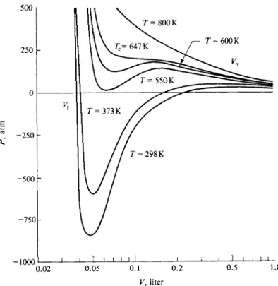
series of values of V. The isotherms of Fig. 1-12 were computed by this procedure for water with a = 5.72 liter2 atm m o l e-2 and b = 0.0319 liter m o l e- 1. (See the next section for a discussion of the problem of choosing van der Waals constants.)

1-9 THE VAN DER WAALS EQUATION 21

V, liter

FIG. 1-12. Isotherms calculated from the van der Waals equation (a = 5.72 liter2 atm mole~2, b = 0.0319 liter mole'1^).

The most obvious aspect of Fig. 1-12 is that many of the isotherms show a maximum and a minimum; this is to be expected since Eq. (1-43) [or (1-49)] is a cubic equation in volume:

P F3 - (Pb + RT) V2 + aV - ab = 0. (1-50)

For a given Ρ there should in general be three roots or values of V. However, for any given choice of a and b there will be a particular value of Τ for which these three roots become equal. Above this value of Τ two roots become imaginary, leaving one real root. At high temperatures, then, the isotherms of Fig. 1-12 look much like Fig. 1-8 for a real substance. The problem is to rationalize the region showing a maximum and a minimum in Fig. 1-12 with the region showing a hori­

zontal line in Fig. 1-8. This is done as follows.

For a real substance isothermal compression across the flat portion of an iso­

therm corresponds to conversion of vapor to liquid at constant pressure. The amount of mechanical work done, as in the piston and cylinder arrangement of Fig. 1-7, is given by

w = work = Γν PdV. (1-51)

J y ι

Notice that if a piston under pressure Ρ sweeps a volume dV, then, as shown in the figure, the total force acting on the piston is / = Ps/ and this force acts through a distance dx, where dV = s/ dx. Thus the integral of Eq. (1-51) corresponds to Sx[ f dx and indeed gives the work done. The limits of integration for Eq. (1-51)

are from the molar volume of the vapor when condensation just starts, Vv , to the molar volume of the liquid when condensation is just completed, Vx. Since P°

is constant, the work is just

w=P»(Vv- Vl). (1-52)

We turn now to the van der Waals equation; referring to Fig. 1-12, it seems clear that the section labeled Vv must represent the molar volume of the gaseous state of the substance, while that labeled Vt should correspond to the liquid state. The van der Waals equation connects these two branches with the section showing a maximum and a minimum, but a real substance takes the short cut of direct condensation when Ρ reaches P° as illustrated in Fig. 1-13. We would like to know how to locate the horizontal line of this short cut, and hence the liquid vapor pressure P°.

We can regard the route taken by the van der Waals equation and that given by the short cut as alternate paths requiring the same amount of work. That is, we require the integral \\r\P dV to be the same along the curved path abed in Fig. 1-13 and along the straight-line path ad,

w = p\vv - vl) = \Vl PdV (curve). (1-53) Graphically, this amounts to equating the two differently shaded areas in the figure;

it also amounts to requiring that the net area between the line ad and the curve abed be zero. Figure 1-14 repeats Fig. 1-12, but with horizontal lines added, as located by the preceding criterion. It is thus possible to interpret the van der Waals equation so as to obtain liquid vapor pressures or P° values.

There are some further interesting aspects to the above considerations. The section abed of the van der Waals isotherm of Fig. 1-13 represents an unstable situation. Thus along the portion ab the pressure of the vapor is greater than the

200

1-9 THE VAN DER WAALS EQUATION 23

0 0.2 0.4 0.6 V, liter

FIG. 1-14. Figure 1-12 with condensation lines added.

condensation pressure for the liquid state. It is actually possible to compress vapors beyond the condensation pressure; the system is unstable toward conden­

sation, but if the vapor is free of dust, the first appearance of liquid droplets may be delayed. The effect is known as supersaturation and occurs because a small liquid drop has a higher vapor pressure than does the bulk liquid, by virtue of having a large surface-to-volume ratio and consequently an appreciable added energy due to the surface energy. The section dc is also metastable ; here liquid is under less pressure than its vapor pressure and should spontaneously form vapor bubbles. Liquid surrounding a small cavity exerts a lower vapor pressure than normal, however, again because of a surface tension effect. This relationship con­

necting size of droplet or bubble, surface tension, and vapor pressure is given by the Kelvin equation, discussed in Section 8-9.

As a further point note that in Fig. 1-12 the lowest van der Waals isotherm reaches negative pressures. The implication is that a liquid can exist under tension, as a metastable condition. This, too, has been verified, and for water a tensile strength of as much as 100 atm has been found (see Commentary and Notes section). Finally, the section be must represent a totally unstable region as opposed to a metastable one, since it calls for volume to increase with increasing pressure.

The van der Waals equation, although fairly simple algebraically, thus describes not only nonideal gas behavior, but also condensation and regions of vapor and liquid metastability; and, of course, it can be used for calculation of the coefficients of compressibility and thermal expansion for both liquids and gases. As discussed in the following section it also predicts critical phenomena and is consistent with the principle of corresponding states. The simplicity of the equation, the wide range of properties which can be treated, and the rather straightforward physical meaning assigned to the a and b constants have combined to make the van der Waals equation by far the one most commonly used in approximate applications.

1-10 The van der Waals Equation, Critical

Phenomena, and the Principle of Corresponding States

As noted in the preceding section, for a given set of a and b values there will be one single temperature at which the van der Waals equation will have three equal roots. At this temperature the equivalent straight-line section will have diminished to a point; this is the critical temperature for a van der Waals substance. The van der Waals critical point may be related to the a and b constants. Perhaps the most convenient way is as follows. At the point of three equal roots the maxima and minima must have just merged. This means that at this point the isotherm for TQ must be horizontal and, moreover, have an inflection point (as illustrated in Fig.

1-12).

The mathematical statements of these conditions are that (dP/dV)T = 0 and (d2P/8V2)T = 0. On applying the indicated differentiations to Eq. (1-49), we have

ί^Λ = -RT, 2a_ = Q

\dVfT (Vc - bf ^ Vc3' K '

l*L\ = 2RT= C _6a_ Q On solving Eqs. (1-49), (1-54), and (1-55) simultaneously we find

Alternatively, we have

b

= Jp7>

-64FT-

"

Finally, the expressions for Vc , Pc , and Tc may be combined to give

PCVC = IRTc. (1-58)

The van der Waals equation also conforms to the principle of corresponding states. From Eqs. (1-56), Ρ = (a/27b2) Ρτ, V = 3bVT , and Τ = ($a/27bR) Tr, and substitution into the van der Waals equation (1-43) then yields

( α + ι| γ) ( ^ - 5 ) = 5γ' · ( 1-5 9) As required by Eq. (1-41), we now have a relationship connecting VT , PT , and TT

which contains no constants specific to the particular substance.

Table 1-5 gives pairs of van der Waals constants for a number of substances.

Different sources give somewhat different values for these constants, however.

They may be obtained in various ways. One is from the critical constants, with Eqs. (1-56). Another is by a best fitting of the van der Waals equation to the gas (as opposed to the vapor) portion of the compressibility chart of Fig. 1-10. The constants can also be obtained from the coefficients of compressibility and thermal expansion for a liquid, and so on. Since the van der Waals equation is still only an approximate equation, each method will yield somewhat different a and b values.

Any one set will then be best suited for calculations around that region of condi-

COMMENTARY AND NOTES 25

TABLE 1-5. Van der Waals Constants for Gasesa

Substance

a

(liter2 ^{atm mole}- 2⁾ (liter mole^b - 1)

He 0.03412 0.02370

Ne 0.2107 0.01709

H2 0.2444 0.02661

o2 ^1.360 0.03183

N2 1.390 0.03913

Cl2 6.493 0.05622

CO 1.485 0.03985

NO 1.340 0.02789

c o2 ^3.592 0.04267

H20 5.464 0.03049

N H3 ^4.170 0.03707

CH4 2.253 0.04278

C2H2 4.390 0.05136

C2H4 4.471 0.05714

C2H6 5.489 0.06380

CH3OH 9.523 0.06702

C2H5OH 12.02 0.08407

C H 3 C O O H 17.59 0.1068

C6H6 18.00 0.1154

0 Landolt-Bornstein, "Physical Chemistry Tables." Springer, Berlin, 1923.

tions for which the set was obtained and will be apt to give poor results when used in calculations for some quite different pressure and temperature region.

As an example, the a and b values for water used in calculating Fig. 1-12 give a good fit to P-V-Tdata for water well above its critical temperature and pressure.

They are appreciably different from the ones calculated from the critical point for water (since Vc is 55 c m3 m o l e- 1, this would give b = 18.5 c m3 as compared to 31.9 c m3 used for Fig. 1-12). One result is that while one would expect the 25°C curve of Fig. 1-12 to cross the Ρ = 0 line at about 18 c m3 m o l e- 1, the molar volume of liquid water, the calculated curve does so at 31.9 c m3 m o l e- 1. Clearly, a different set of a and b values would better represent this region of the P-V-T plot for water. It is as a consequence of such quantitative deficiencies of the van der Waals equation that various more elaborate analytical equations of state have been proposed. Some of these are mentioned in the Commentary and Notes section.

COMMENTARY AND NOTES

A section of this type occurs at the end of the main portion of most chapters.

The purposes are, first, to provide some qualitative commentary on interesting but less central aspects of the chapter material and, second, to supply, for reference purposes, additional quantitative results. The latter will ordinarily be presented without derivation or much discussion.

There are, for example, a number of other semiempirical equations of state that have found use. Some of these are

Clausius equation:

[

nv^wY

~ =

- ^

Berthelot equation:

(ρ +

-JL^yV

P(V - b) = RTe~alRTV. (1-62)

Beattie-Bridgman equation:

P= v7R€) i V + B ) - ±T ( l 9 (1-63) where A = A0[l + (α/Κ)], Β = B0[l - (b/V)], and e = c/VT\ and A0 and B0 are

constants.

Benson-Golding equation:

(' + -y^f^Y

~

~

=

'

"

(See Glasstone, 1946; Weston, 1950; Benson and Golding, 1951.)

These equations tend to be of the form of the van der Waals equation, but with improvements designed to allow for a temperature dependence of a and b. The Beattie-Bridgman equation was designed for gases at high pressures.

Some of the various properties that an equation of state should in principle be able to predict were mentioned in the discussion of the van der Waals equation.

A brief elaboration is worthwhile. For example, the idea of a tensile strength for a liquid may seem unexpected. The experimental problem, of course, is that one cannot simply pull on a column of liquid as one might on a rod of solid material.

What one actually does is to fill a capillary tube with liquid at some elevated temperature and then seal the tube. On cooling, the liquid should contract, but to do so a bubble of vapor would have to form, and if the liquid is free of dust or if the cooling is rapid enough, the column of liquid remains intact and therefore under tension. One calculates this tension from the coefficient of compressibility, knowing how much the liquid has been forced to expand in order to keep filling the capillary at the lower temperature. Negative pressure may be applied mechani­

cally, but less easily. This situation does occur, however, with a boat propeller;

liquid behind the rotating blades is momentarily under tension. An important practical problem is to avoid cavitation, or the formation of vapor bubbles; the sudden collapse of such bubbles not only hampers the propeller but can pluck out metal grains to roughen and eventually destroy the surface.

Another property which can be calculated from an equation of state is the surface tension of a liquid. We ordinarily think of pressure as a scalar or non- directional quantity, but in the case of a crystalline, nonisotropic solid, application of a uniform pressure will distort the crystal. To avoid this, we would have to exert different pressures on each crystal face. In general, then, pressure can be treated as a set of stresses or directional vectors.

COMMENTARY AND NOTES 27

Since a liquid does not support stress, the pressure around any portion of a liquid must be isotropic. This is not true, however, in the surface region. The pressure normal to the surface must indeed be the same as the general pressure throughout the system. However, the pressure parallel to the surface varies through the inter­

face. Analysis shows that the surface tension y can be calculated if the difference between the pressure normal to the surface and that parallel to the surface is known as a function of distance through the interface. The equation is

where Ρ is the general, isotropic pressure, ρ is the local pressure component parallel to the surface, and χ is distance normal to the surface. If we can, by some analysis, calculate how the density or molar volume varies across a liquid-vapor interface, then use of an equation of state such as the van der Waals equation allows a calculation of ρ as a function of x, and hence of the surface tension (see Tolman, 1949).

A final brief consideration concerns the determination of the critical point of a substance. The reality of a critical point can be seen by means of the following type of experiment. A capillary tube is evacuated and then partly filled with liquid, the remaining space containing no foreign gases but only vapor of the substance in question; the tube is then sealed. On heating, opposing changes take place. The liquid phase increases its vapor pressure, and the vapor density increases as vapori­

zation occurs; this acts to diminish the volume of liquid phase. On the other hand, the liquid itself expands on heating. If just the proper degree of filling of the capil­

lary was achieved, these two effects will approximately balance, and the liquid- vapor meniscus will remain virtually fixed in position as the capillary is heated.

A temperature will then be reached at which the meniscus begins to become diffuse and then no longer visible as a dividing surface. At this temperature the system often shows opalescence; the vapor and liquid densities are so nearly the same and their energy difference is so small that fluctuations can produce transient large liquidlike aggregates in the vapor and vice versa in the liquid. There is still an average density gradient. However, at a slightly higher temperature, perhaps 5-10 Κ more, the system becomes essentially uniform. This last is the critical temperature; knowing the amount of substance and the volume of the capillary, one also knows the critical molar volume.

This type of visual experiment, although quite interesting, does not allow a very precise determination of the critical point. An alternative procedure makes use of a series of isotherms such as are shown in Fig. 1-8. However, while the broken line joining the end points of the condensation lines can be fairly well established, its exact maximum point is hard to fix exactly. This locus may alternatively be plotted as temperature versus the equilibrium vapor and liquid densities pv and px ^as illustrated in Fig. 1-15. A useful observation, known as the law of the rectilinear diameter, states that the average density / oav = (pi + />v)/2 is a linear function of temperature, as also illustrated in the figure. The essentially straight and nearly vertical line of pav versus Τ makes an easily defined intersection with the curved line of densities. This intersection then gives the critical temperature and density.

.liquid phase

(P - p) dx, (1-65) vapor phase

\ \

) 0.2 0.4 0.6 0.8 p, g c m-3

FIG. 1-15. Illustration of the law of the rectilinear diameter.

SPECIAL TOPICS

The Special Topics section at the end of each chapter takes up either more specialized or more advanced aspects of the chapter material. The intention is to provide a section, separated from the main body of material, which can be con­

sidered if time in the course permits, or as self-study on the part of the interested student. Although the material in the main body of succeeding chapters will not draw on previous Special Topics sections, subsequent Special Topics sections may make use of the results of preceding ones.

The van der Waals and other equations of state cited in this chapter are illustra­

tions of a semiempirical approach in which the goal is to obtain a definite functional form for the equation of state. Contemporary theoretical chemists now pursue the line of using a detailed expression for the intermolecular potential between two molecules to obtain values for the virial coefficients of Eq. (1-37) The potential function will be somewhat approximate or semiempirical, but the ensuing and generally quite elaborate theoretical development may be rigorous.

If the mutual potential energy between two molecules as a function of the sepa­

ration r is denoted by <£(r), then a statistical mechanical derivation, which is beyond the scope of this text, gives the following equation for the second virial coefficient (see Hirschfelder et al, 1954):

B(T) = 2πΝ0 Γ (1 - e-+wikT) r2 dr, (1-66)

J ο where N0 is Avogadro's number.

A very qualitative rationale of the treatment is as follows. It was noted in Section 1-5 that the barometric equation could be regarded as a particular appli­

cation of the Boltzmann principle Eq. (1-35). The principle stated that the probab­

ility of a molecule having an energy e is proportional to e~^kT.