CHAPTER NINE
SOLUTIONS OF NONELECTROLYTES
9-1 Introduction
We introduce, with this chapter, the physical chemistry of systems for which composition is a state variable. A solution is a mixture at the molecular level of two or more chemical species; it may be gaseous, liquid, or solid. If clusters of molecules are present, the situation becomes more complex. If the clusters are of the order of 100  to a few thousand  or around 10" 4 cm in size, the system is colloidal in nature. If they reach to 1 0 "4 to 1 0 "3 cm, we speak of the mixture as a suspension, an emulsion, or an aerosol. Beyond this, we simply have a mechanical mixture of two or more bulk phases.
There are no sharp natural boundaries in this sequence, but there are practical ones. Most physical chemists have concentrated on the extremes, that is, on mole
cular solutions or on systems having well-defined bulk phases which themselves may be solutions. On the other hand, much of the biological and physical world involves mixtures of the colloidal or intermediate type of dispersity. The physical chemistry of these last systems is difficult, and its introduction is reserved for Chapter 21. We confine ourselves here to the simpler case of molecular solutions.
A solution or mixture of gases presents little problem, at least at the level of complexity of this text. Unless very dense, gases are always fully miscible and, in the usual laboratory pressure range of around 1 atm, form essentially ideal solutions. Dalton's law of partial pressures [Eq. (1-18)] is well obeyed. We will consider the entropy and free energy of formation of gaseous mixtures in Section 9-4.
Solid solutions, that is, molecular dispersions of two or more species in a solid phase, are quite common. Alloys are one example; also, many ionic crystals are able to substitute one type of ion for another (of the same charge) almost randomly within their crystal lattices. Solid solutions are more difficult to study experi
mentally, however, and are less studied than liquid ones. Their behavior is also more subject to eccentricities. Most of our data are from, and most of our common experience is with, liquid solutions. For these reasons, the material that follows
301
refers mainly to liquid solutions. It should be remembered, however, that the formal thermodynamics is the same for both types of solutions.
It is now desirable to define the term composition more precisely. A phase may consist of a number of molecular species and yet still qualify thermodynamically as a pure substance. Liquid water, for example, contains not only a large assortment of transient clusters (see Section 8-CN-2), but also definite concentrations of hydrogen and hydroxide ions. These are all in equilibrium with each other, however, and their relative proportions are not subject to arbitrary change. Composition with respect to these species is not an independent variable; once we fix the temperature and pressure of a sample of water, we automatically also fix the various equilibrium constants and hence compositions. It is therefore not necessarily the number of species present that serves to characterize a solution. Nor is it necessarily the number of constituents. By constituents, we mean chemical species that we can physically measure out in making up a solution. The term formal composition denotes the composition calculated in terms of what is weighed out and mixed.
We may, for example, prepare a mixture of hydrogen, nitrogen, and ammonia.
In the presence of a catalyst, these would be in equilibrium, and it would be suffi
cient to specify the formal composition with respect to only two of the three species. In the absence of the catalyst, however, all three compositions are inde
pendently variable, and the formal composition with respect to all three would have to be specified.
We meet this type of complication by using the term component. The number of components of a solution (or of any mixture) is the least number of independently variable chemical species required to define the composition of the solution (and of all phases present, if there is more than one). Hydrogen plus nitrogen plus ammonia plus catalyst is a two-component system; without the catalyst, it becomes a three-component system. Ordinary water is a one-component system; water plus solute is a two-component system, and so forth.
As to compositions themselves, various measures are used. A common one for this chapter will be the mole fraction, denoted by x{ for a liquid solution and, for clarity, by y{ for a gaseous solution. Mole fractions are strictly additive. That is, the total number of moles of a solution is just the sum of the numbers of moles of each species, and the mole fraction composition of a solution formed when two others are mixed is strictly obtainable on this basis. Volume fractions φ{ are sometimes used, but the volume of a solution is not in general equal to the sum of the volumes of the constituents mixed, and care must be taken in the definition of the exact experimental basis for a volume fraction.
The term molality, m, denotes a kind of mole fraction which is well suited to aqueous solutions. It means the number of moles of the dilute or solute compo
nent per 1000 g of the major or solvent component. Finally, it is convenient both for the laboratory chemist and in certain theoretical treatments to use volume concentration. The term molarity, M, will be used here to denote moles per liter of solution (not of solvent alone), and η to denote the rational concentration unit of molecules per cubic centimeter of solution.
Finally, we will deal with solutions mainly from the phenomenological or classical thermodynamic point of view. Much formal statistical thermodynamics has been developed for solutions, but the complications are such that this approach is not as yet a powerful one in actual application. The statistical thermodynamic point of view is therefore discussed only briefly, in the Commentary and Notes section.
9-2 THE VAPOR PRESSURE OF SOLUTIONS. RAOULT'S AND HENRY'S LAWS 303
9-2 The Vapor Pressure of Solutions. Raoult's and Henry's Laws
The vapor pressure and vapor composition in equilibrium with a solution of volatile substances constitute important and very useful information. The practical usefulness lies in the application to distillation processes, and the physical chemical importance, in the provision of a means of studying the thermodynamic properties of liquids and of testing models for the structure of liquids. One function of this section is therefore to introduce characteristic data and behavior as a preliminary to the thermodynamic treatments.
A. Vapor Pressure Diagrams
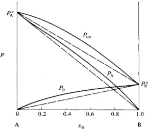
Vapor pressure data are customarily displayed in the form of vapor pressure- composition diagrams for some particular temperature, as illustrated schematically in Fig. 9-1. Here Ptot is the total combined vapor pressure above varying compo-
0 0.2 0.4 0.6 0.8 1.0
FIG. 9 - 1 . Vapor pressure-composition diagram.
sitions of a solution of liquids A and B. The liquids are, in this example, taken to be fairly similar, and the Ptot curve, although not linear, decreases steadily from PA° , the vapor pressure of pure A, to PB° , that of pure B, as xB is varied from 0 to 1. The vapor is a mixture of gaseous A and B, and the variations of the partial pressures PA and PB are also shown. We assume that no other gases are present and that the vapors are ideal, so that
PU*=PA+PB. (9-1)
If A and Β are very similar, the limiting case being one of two substances differing only in isotopic content, then the vapor pressure diagram takes on an especially simple appearance. A good example is provided by the benzene-toluene system, shown in Fig. 9-2. The values of Ptot, Pb , and Pt are now given by nearly
0 0.2 0.4 0.6 0.8 1.0
Benzene xt Toluene
(b)
F I G . 9-2. The benzene-toluene system at 20°C: (a) vapor pressure-liquid composition diagram;
(b) liquid and vapor composition diagram.
straight lines. Thus we have
Pt = Pt°xu Pb = Pb°(l - xt) = i V x b , (9-2) where xt and XD denote the mole fractions of toluene and of benzene, respectively,
and the degree superscript indicates a pure phase. Then Ptot is simply
Ptot = Pt + Pb = Pb° + (Pt° - Pb°) x t , (9-3) which is the equation of the straight line connecting Pb° with Pt° . A solution with
this behavior is called an ideal solution, and the general form corresponding to Eqs. (9-2) is called Raoulfs law (1884):
Pi = Pi°Xi · (9-4)
For simplicity, we will largely restrict the discussion to two-component systems, for which the Raoult's law statements are
Ρ, = P1°x1, P2 = P2°x2, (9-5)
9-2 THE VAPOR PRESSURE OF SOLUTIONS. RAOULFS AND HENRY'S LAWS 305
with the corollary that
Ptot = Λ ° + ( Λ ° - Pi) *2 · (9-6)
As will be seen in the Commentary and Notes section, Raoult's law corresponds to a particularly simple picture of a solution—essentially one in which the com
ponents are distinguishable, but just barely, so that their physical properties are virtually identical. The situation is rather analogous to that of the ideal gas; the ideal gas law also corresponds to a particular, very simple picture. The ideal gas law is, moreover, the limiting law for all real gases, and, in this respect, is not hypothetical or approximate at all. The same is believed to be true for Raoult's law. Experimental evidence suggests that Raoult's law is the limiting law for all
400 r
400 r
Η ο
0 0.2 Acetone
0.8 1.0 Chloroform
F I G . 9 - 3 . The acetone-chloroform system at 35°C, showing negative deviation from ideality;
(a) vapor pressure-liquid composition diagram; (b) liquid and vapor composition diagram.
solutions, approached by each component as its mole fraction approaches unity.
That is, as a limiting law statement, Eq. (9-4) reads
Notice that the curves for PA and PB are drawn in Fig. 9-1 so that they approach the Raoult's law line as xA and xB approach unity. The acetone-chloro
form system shown in Fig. 9-3 provides a specific illustration. In this case, the partial pressure curves lie below the Raoult's law lines, whereas in Fig. 9-1, they lie above the Raoult's law lines. We speak of the first situation as one of negative deviation, and the second, as one of positive deviation (from ideality).
Raoult's law as an ideal law is easy to understand theoretically. It is the expected behavior if there is complete uniformity of intermolecular forces, just as the ideal gas law is the expected behavior in the complete absence of intermolecular forces.
Raoult's law as a limiting law, Eq. (9-7), is a statement of experimental observation.
While we assume that it is the limiting law for all systems, there is no rigorous theoretical proof. By contrast, the ideal gas law can be shown to be the expected limiting law for all real gases.
Acceptance of Raoult's limiting law provides a basis for the understanding of a second limiting law, Henry's law. Henry's law states that the partial pressure of a component becomes proportional to its mole fraction in the limit of zero con
centration:
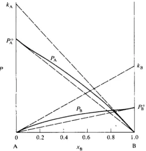
This is illustrated in Fig. 9-4, in which the vapor pressure curves of Fig. 9-1 are shown approaching the limiting slopes kA and kB ; these slopes define straight lines whose intercepts are kA and kB . Under the limiting Henry's law condition each molecule of component A has become surrounded by Β molecules. The environment is thus not one of pure A, but another environment determined by
lim Pt = P , ° x , . (9-7)
(9-8)
ρ
0 0.2 0.4 0.6 0.8 1.0
A Β
FIG. 9 - 4 . System showing positive deviation from ideality; illustration of Henry's and Raoult's laws.
9-2 THE VAPOR PRESSURE OF SOLUTIONS. RAOULT'S AND HENRY'S LAWS 307
the nature of the A - B interactions. We can regard kA as the hypothetical vapor pressure that pure A would exert if the molecules all had this different environment, and similarly, kB as the hypothetical vapor pressure that pure Β would exert in an environment consisting of A molecules.
Like Raoult's law, Henry's law applies as a limiting law to systems of both positive and negative deviation from ideality. The partial pressure curves in Figs. 9-3 and 9-4 obey both limiting laws.
B. Solubility of Gases
Henry's law is approximately valid for any solute in a dilute solution, and a particular application is to the solubility of gases in liquids. As an approximate law, Eq. (9-8) becomes
Ρ2 = k2x2, (9-9)
where species 2 in a two-component system will, by convention, be taken to refer to the solute. The solubilities of permanent, inert gases (such as N2, 02, CO, and C H4) in water at 25°C give k2 values of ~ 1 05 atm. Thus k2 is 0.426 X 10⁵ atm for 02 in water; the solubility is then xÛ2 = 1/(0.42 6 χ 105) = 2.35 χ 1 0 "5 at
1 atm. Since there are 55.5 moles of water per liter, this solubility corresponds to 1.30 χ 10" 3 M per atm at 25°C. The partial pressure of oxygen in air is 0.2 atm, so the actual concentration, due to equilibration with air, is (1.30 χ 10"3)(0.2) = 2.61 X 1 0 "4 M. In this case, there will also be dissolved nitrogen present, corre
sponding to its k2 value of 0.86 χ 105 atm.
Some of the literature report Henry's law constants for gases in terms of the volume of gas dissolved, measured at the temperature and pressure in question, per unit volume of solvent. The Henry's law constant for oxygen becomes, on
this basis, (1.30 X 10"3)(0.082)(298)/1.0 or 0.032 liter of 02 per liter of water.
C. Vapor Composition Diagrams
A vapor pressure diagram also contains the information to give the composition of the vapor in equilibrium with a given composition of solution. Thus, for the system of Fig. 9-1, we have
"-fc-FTfr-.-
Λ~ £ - ? 3 * · <>-'°>
where yA and vB denote the mole fractions of A and Β in the vapor, respectively.
A conventional way of supplying this information is to plot the vapor composition corresponding to each value of Ptot, along with Ptot versus liquid composition, as shown in Fig. 9-5. For example, for a liquid of composition xx, Ptot has the value Ρλ, and the solution is in equilibrium with vapor of composition y1. The corre
sponding vapor composition plots are included in Figs. 9-2(b) and 9-3(b).
Vapor composition diagrams are in effect phase maps or phase diagrams. If the system is contained in a piston and cylinder arrangement thermostated to the given temperature, then from Fig. 9-5, liquid of composition x1 cannot vaporize if the pressure is greater than Px ; the system will consist of liquid phase only. The same
0 yx y2 χχ x2 1
^3
Α χβ Β
F I G . 9-5. Use of vapor pressure and vapor composition diagrams—the lever principle.
will be true for any composition and pressure defining a point lying above the liquid line. The upper region of the diagram is one of liquid phase only. Similarly, a system of composition xx at a pressure less than Pz will consist of vapor phase only. The lower region of the diagram must be one of vapor phase only. The liquid and vapor composition lines thus mark the boundaries of the liquid-only and vapor- only regions, respectively. Finally, a system whose overall composition and pressure locate a point between the two lines will consist of a mixture of phases.
A diagram such as that of Fig. 9-5 allows a complete tracing of the sequence of events as the pressure of a system is changed at constant temperature. Suppose, for example, that a system of composition χτ is initially under some high pressure. As the pressure is reduced vaporization will begin at Ρλ, producing vapor of compo
sition y1. With further decrease in pressure more and more vaporization must occur, and since the vapor is richer in A than is the liquid, the latter must move to the right in composition. When the pressure has reached P2, liquid of composition x2 is now in equilibrium with vapor of composition y2. Finally, when the pressure has been reduced to P3 all the liquid will be vaporized and further reduction in pressure will merely expand the mixed vapors.
Since the entire system is a closed one, the vapor and liquid phases are always of some uniform relative composition, and their relative amounts can be calculated by material balance. For example, if the system consists of η moles total, then at any point
n=ny + nl9 (9-11)
where nx and nv are the number of moles of liquid phase and of vapor phase, respectively. Thus for a system of overall composition xx and at pressure P2 the material balance in Β is
nx1 = nvy2 + nxx2 = nvy2 + (n — nv) x2. (9-12)
9-2 THE VAPOR PRESSURE OF SOLUTIONS. RAOULT'S AND HENRY'S LAWS 309 Equation (9-12) rearranges to give
Λ ν = * 2 - * i _1) 3 ( 9
η x2 — y2
Equation (9-13) can be given a very simple and useful graphical interpretation.
The horizontal line connecting the points y2 and x2 is known as a tie-line. In general a tie-line connects the compositions of equilibrium phases. The difference x2 — y2 corresponds to the length of the tie-line at P2 and the difference x2 — xl9 the length of the right-hand section of the line. Alternatively, if the tie-line is regarded as a balance pivoted at the point χλ, then weights proportional to nY and nx will just balance if placed at the y2 and x2 ends, respectively. Equation (9-13) with its associated graphical interpretation is known as the lever principle.
D. Maximum and Minimum Vapor Pressure Diagrams
The acetone-chloroform system of Fig. 9-3 shows a minimum in i\ o t · The physical interpretation is along the lines of Fig. 8-5, where for a pure liquid the energy of vaporization was attributed to ηφ/2, where η is the number of nearest neighbors and φ is the interaction energy. A negative deviation then suggests that ΦΑΒ is greater than φΑΑ or φΒΒ , so that the ease of vaporization is reduced if A and Β molecules mutally surround each other.
Such an increase in interaction energy between unlike molecules would, as an extreme, lead to the formation of an actual compound. In the case of Fig. 9-3 the appearance is more that of a tendency toward association. The fact that the deviation of Ptot from the ideal or Raoult's law line is at a maximum at about 50 % mole fraction suggests that the association is of the AB type (and not A2B or A B2, and so on).
The extreme case, in terms of this picture, would be one in which a very stable AB compound actually formed, as illustrated in Fig. 9-6. Systems in which the overall composition xB is less than 0.5 consist of a solution of A and AB, those of
A A B Β A A B Β
(a) (b) FIG. 9 - 6 . Formation of a stable compound AB, but with the solutions A + AB and Β + AB
ideal.
200
150 ο
100 h
ο 0.2 0.4 0.6 0.8 1.0
Benzene Ethanol
F I G . 9 - 7 . The benzene-ethanol system at 35°C.
composition greater than 0.5 consist of a solution of Β and AB. These two solutions are shown as ideal but need not be. Note that there is a discontinuity in the slope of the Ptot line at xB = 0.5. In the acetone-chloroform system, however, the Ptot line is rounded at the minimum—an indication that no very stable AB complex forms. One may, in fact, estimate the dissociation constant of such a complex from the degree of curvature around this minimum.
Deviations from ideality may, of course, be positive. This is illustrated in Fig. 9-7 for the system benzene-ethanol. The physical argument is now reversed; we con
clude that φΑΒ is less than φΑΑ or φΒΒ . The extreme of this situation is that in which the two liquids have limited solubility in each other. This means that two phases a and β of different composition can coexist, and that therefore
= V = PÎ, = V = Pf, Ρ = PA + PB , (9-14) where the superscript α or β refers to a quantity for a single phase and the super
script αβ stands for a quantity when both phases are present.
The limiting situation of complete immiscibility is shown in Fig. 9-8. The pos
sible types of sequences are those for the systems x2 and xx. All systems now consist of two liquid phases initially, and when the pressure is reduced to PAB vapor phase of composition yAB forms and continues to do so until one liquid or the other is gone. The remaining liquid then continues to vaporize along the appropriate vapor composition line. The composition yAB is in this case given by
y ,ΑΒ
PA° + PB° (9-15)
£. A Model for Nonideal Solutions
A fairly simple treatment developed by M. Margules in 1895 is still a very useful one. The difference between φΑΒ and φΑΑ can be regarded as an energy term which
9-2 THE VAPOR PRESSURE OF SOLUTIONS. RAOULT'S AND HENRY'S LAWS 311
enters as a Boltzmann factor modifying PA over its ideal value. This energy difference should be approximately proportional to xB2 on the basis of arguments about the proportion of Α - A and A - B interactions, and one writes
PA = PA°XA exp(axB2), ( 9 -1 6)
where a: is a characteristic constant (and is temperature-dependent). Since the A - B interaction is a mutual one, a similar equation applies to PB :
PB = PB°XB e x p( c u tA2) , (9-17)
where a is the same constant as in Eq. (9-16). Notice the Eqs. (9-16) and (9-17) give Raoult's law as a limiting law, and reduce to Raoult's law for all compositions if oc = 0.
The model also provides a relationship between the Henry's law constants kA and kB [Eq. (9-8)]. Thus from Eq. (9-16) we have
dP
^ = iV[exp(ax
B2)](l -
2axAxB) (9-18)and in the limit when xA —> 0,
kA = PA°e«. (9-19)
The situation is symmetric, and so
kB = PB°e\ (9-20)
Thus the two Henry's law constants are predicted to be in the ratio of the P°
values. This rule is obeyed reasonably well except for strongly associated liquids (a very negative).
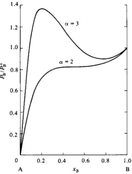
In the case of positive deviation oc is positive, and if sufficiently so, the curve calculated from Eq. (9-17) will show a maximum and a minimum, as illustrated in Fig. 9-9. The situation is reminiscent of that with respect to the van der Waals
1.4
1.2
1.0
°CQ
Ï 0. 8 0?
0.6
0.4
0.2
0 0. 2 0. 4 0. 6 0. 8 1. 0
A xB Β
FIG. 9 - 9 . Plot of Ρ Β according to the Mar gules equation (9-17). (The plot of PA is similar, but increases from right to left, of course.)
equation and the conclusion is that the experimental vapor pressure curve must show an equivalent horizontal portion and that the system is one of partial miscibility. The "critical temperature" is such that α = 2. For this value of OL the system just fails to show a miscibility gap.
9-3 The Thermodynamics of Multicomponent Systems
Some aspects of the more formal thermodynamics of solutions, gaseous, liquid, or solid, must now be taken up. An important result will be the introduction of a new quantity, the chemical potential, which plays much the same role for solutions as G does for pure substances. The criterion for phase equilibrium is then expanded to the case of phases that are solutions, and an important new relationship, the Gibbs-Duhem equation, is introduced. Further developments are given in the Special Topics section, including the thermodynamic treatment of the surface tension of solutions. The principal new concept to be understood is that of partial molal quantities. Thermodynamics has become more complicated, but unavoidably so.
A. The Chemical Potential
The various thermodynamic functions must now include the amount of each component as a variable. That is, we consider what is called an open system, or one which may gain or lose chemical species. Thus the total energy Ε is a function of S, v9 and now nt, where n{ denotes the number of moles of the ith species, and
9-3 THE THERMODYNAMICS OF MULTICOMPONENT SYSTEMS 313
sans serif (E, S, and so on) denotes extensive quantities not on a per mole basis. The total differential for Ε is
* - ( $ . . * + ( ϊ ) . * + ( £ ) , , , * . + - ·
(9-21) Comparison with Eq. (6-12), to which Eq. (9-21) should reduce if the dnt are zero, givesf
dE = TdS —Pdv + 2 ( ^ p ) Λι. · (9-22)
Similarly, free energy is now a function of Τ, P , and also nt, so we have
Comparison with Eq. (6-43) identifies the first two coefficients, so that
dG = -SdT+vdP + Σ (-g^-) · (9-24)
Alternatively, however, we have
rfG = dH - d(TS) = dE + Ρ dv + ν dP - TdS - S dT, (9-25) so, in combination with Eq. (9-22), it must also be true that
dG = -SdT + vdP + l ( S3E_ - ) ^ - (9-26) Thus we have
0E \ I dG
μί ( dnt )s.v
(
dnt )t,p : (9-27)where μι is a new quantity called the chemical potential.
Equations (9-22) and (9-26) can now be written
dE = TdS - Ρ dv + Σ Pi a n ,, (9-28)
i
dG = - S dT + ν dP + £ μί dn{. (9-29)
i
The second of these is perhaps the more useful since it identifies the chemical potential μί as the free energy change of a system per mole of added component /, with temperature, pressure, and the other mole quantities kept constant. The chemical potential is a coefficient (like heat capacity) and we are really talking about the change dG for a small increment dn{. The added amount of the zth
+ To simplify the appearance of equations, the reminder η, φ nt will be taken for granted in derivatives such as (dG/d/if)s,v,n/*nf»
component should not be sufficient to change the composition of the system appreciably since μ{ will depend on composition as well as on temperature and pressure.
β . Partial M o / a / Quantities
The chemical potential is one of a family of partial molal quantities. If, in general, we have some extensive property ^ , then for a solution ^ is the partial molal property for the ith component:
' T.P
Thus
*-(•£•)„· <»'>
"·-(-£)„·
<9-
32)and
Si = ^ ) Ty (9"33)
Further, the various thermodynamic coefficients that were derived for a single substance retain the same form for the ith component of a solution if the corre
sponding partial molal quantities are used. As useful examples, we have
V dP ) T 3P \ drii JPtT drii \ dP ) T \ dn, 1 P>T 1 K ' and, similarly,
Equation (9-34) may be applied to a mixture of ideal gases. By Eq. (9-31), 1 ~ \dnjT,p ~ Ρ \dnJT.p ~~ Ρ '
Then
RT
ΐΒμΛ y RT
\dP)T 1 Ρ
and
din = RT% = RTφ = RTdin Pf (ideal gas) (9-36) since Px = xtP and, under the conditions of the differentiation, dP{ = xt dP{. We thus have
frig) = P>i\g) + RT In Pt (ideal gas), (9-37)
9-3 THE THERMODYNAMICS OF MULTICOMPONENT SYSTEMS 315
where Pi°(g) is the chemical potential of the gas in its standard state, ordinarily taken to be 1 atm. (The same equation applies for a nonideal gas with fugacity fi replacing P{—see Section 6-ST-2.) Since Pi°(g) refers to pure component /, it could just as well have been written Gi°(g); it seems preferable, however, to keep the notation symmetric. [See Robinson (1964) for a discussion of the preceding derivation.]
C. Criterion for Phase Equilibrium
We are dealing with equilibrium systems, and hence with systems for which no spontaneous change in temperature or pressure occurs. Equation (9-29) then reduces to
dG^Z^i dnt · (9-38) i
If the system consists of a single phase and is chemically isolated, that is, if no chemical species can enter or leave, then the criterion for equilibrium given by Eq. (6-42) applies, so we have
dG = 0, Σ μ, dnt = 0. (9-39)
i
Alternatively, the system might consist of two (or more) phases in equilibrium.
For each phase there will be an equation of the form of Eq. (9-38):
dG« = Χ μ? dnf, dG* = Σ μβ dnf, (9-40) i i
and so forth, where
dG = dG- + dG& + ···. (9-41)
If the entire set of phases is in equilibrium and constitutes a chemically closed system overall, then again dG is zero, and we now have
0 = X dnt + Σ an? + · · · . (9-42) i i
Suppose that some process occurs in this equilibrium system of phases whereby dn{ moles of the ith species is transferred from phase a to phase β; all other dn quantities are zero. For this process it follows that
μΐ dn^ + μ/ dnf = 0. (9-43) Since dnt — —dn? (the total number of moles of the ith species remains the same
in the overall system), we have
= μ-i*· (9-44) The very important conclusion is that for phase equilibrium between solutions
the chemical potential of each species must be the same in every phase in which it is present. Equation (9-44) is a more general statement of the equilibrium condition for a pure substance, <?* = GB.
D. The Gibbs-Duhem Equation
A very useful relationship may be obtained from Eq. (9-28). Since our appli
cations will be restricted to two-component systems, we will make the derivation on that basis. The differentials of Eq. (9-28) are all of the form
(intensive property) χ i/(extensive property).
We can therefore imagine that we introduce additional amounts of components 1 and 2, keeping the temperature, pressure, and composition (and hence μ1 and μ2) constant. The result amounts to an integration giving
Ε = TS — Pv + μιηλ + μ2η2. (9-45)
Since
G = Ε + Pv - TS, we can write
G = ηχμχ + η2μ2. (9-46)
Differentiation of Eq. (9-46) gives
dG = nx άμλ + μ1 dn1 + n2 άμ2 + μ2 dn2 (9-47) and comparison with Eq. (9-38) leads to the result
nx άμχ + n2 άμ2 = 0. (9-48)
We divide by the total number of moles to obtain
Jfr άμχ + X2 άμ2 = 0. (9-49)
Equations (9-48) and (9-49) are alternative forms of the Gibbs-Duhem equation.
Its great usefulness is in relating the chemical potential change of one component (for a constant-temperature, constant-pressure process) to that of the other. The next section provides some specific applications.
An alternative way of obtaining Eq. (9-48) is as follows. Equation (9-45) is of general validity and may be differentiated to give
dE = TdS + S dT - Ρ dv - ν dP + μλάηχ + nx άμχ + μ2 dn2 + n2 άμ2. (9-50) Comparison with Eq. (9-28) gives
0 = S dT - ν dP + nx άμλ + n2 άμ2. (9-51) For a process at constant temperature and pressure, Eq. (9-51) reduces to Eq. (9-48).
We will find this type of procedure useful in obtaining the Gibbs adsorption equation (see Special Topics section).
9-4 Ideal Gas Mixtures
The chemical potential of a component of an ideal gas mixture is given by Eq. (9-37),
Μ * ) = ^ ° ( * ) + Λ Γ 1 η Λ .
9-5 ACTIVITIES AND ACTIVITY COEFFICIENTS 317
Gas 1 Gas 2 Mixture at Ρ, Τ at Ρ, Τ at Ρ, Τ
F I G . 9 - 1 0 .
We can apply this equation to calculate the free energy and entropy change for the isothermal process
«i(gas 1 at P) + n2( gas 2 at P)
= mixture (at P, with P1 = xxP and P2 = x2P). (9-52) The process, physically, corresponds to the procedure shown in Fig. 9-10. For pure
gases, G1 = n1^1°(g) +RT In P] and G2 = n2^2{g) + RT In P]. The free energy of the mixture is, by Eq. (9-46),
Gm ix = n^ig) + RTln P J + η2\μ2\έ) + * Γ 1 η Pa] , or, since Px = χλΡ and P2 = x2P, substitution gives
Gm ix = «i[/*i°(g) + RTln Ρ + RTln * J + n2\ji2°(g) + RT In Ρ + RTln x2].
The free energy change for process (9-52) is Gm ix — G1 — G2 or
AGM = nxRT In χλ + n2RT In x2 (ideal gas). (9-53) The free energy of mixing per mole of mixture is
Δ GM = XlRT In x1 + x2RT In x2 (ideal gas). (9-54) Since AS = —[d(AG)/3T]P , the entropy of mixing per mole of solution is
^ S M = —(xiR In xx + x2R In x2) (ideal gas). (9-55) Notice that the free energy of mixing is independent of Ρ and that the entropy of
mixing is independent of both Ρ and T. The latter could have been obtained on the basis of the probability arguments of Section 6-8A (see Commentary and Notes section).
9-5 Ideal and Nonideal Solutions.
Activities and Activity Coefficients
We can apply the criterion for equilibrium to the case of a solution and its vapor. The treatment will be in terms of a liquid solution, but it is equally applicable to solid solutions. The vapor phase is assumed, as usual, to be ideal, and for simplicity we consider only a two-component solution. The requirement that the chemical potential of a component be the same in two phases that are in equi-
librium may be combined with Eq. (9-37) to give
μι(!) = hh(g) = hh°(g) + RTln Px. (9-56)
In the case of a pure liquid μχ{1) becomes μχ(1) [or just Gx°(l)] and Eq. (9-56) reduces to
fJL10(l) = H01(g) + RTlnP1O. (9-57) Alternatively, we may add and subtract RTlnPx° on the right-hand side of
Eq. (9-56) to obtain
j*i(0 = W(g) + RT In Px°] + RT In A . or
hh(l) = μΛΙ)+ RT In (9-58)
We thus have two ways of expressing the chemical potential of component one.
Equation (9-56) does so in terms of μχ°^) and Px, while Eq. (9-58) does so in terms of μχ°(1) and Px/Px°. In the first case the standard or reference state is the vapor at unit pressure, 1 atm, and in the second case it is the pure liquid. The equations are symmetric with respect to the components and so a parallel set of relationships applies for component 2:
μ2(1)= μΜ +RT In P2, (9-59)
to(l) = μΛΟ + RTln A . (9-60)
A. Ideal Solutions
Equations (9-58) and (9-60) take on a very simple form if Raoult's law is obeyed, since then PJP^ = x1 and P2/P2° = x2. Thus
μι(0 = μι°(1) + RTln xx (ideal solution), (9-61) μ2(1) = μ2°{1) + i?71n x2 (ideal solution). (9-62) We can use Eq. (9-46) to obtain the total free energy of the solution:
G = + η2μ2°{ϊ) + nxRT In xx + n2RTIn x2 (ideal solutions). (9-63) If we now consider the process of preparing the solution by mixing the pure liquids,
^(component 1) + «2(c o mPo n e nl 2) = solution, (9-64) the corresponding free energy change is
AGM = nxRT In xx + n2RTIn x2 (ideal solution). (9-65) or, per mole of solution,
AGM = XiRT In xx + x2RTIn x2 (ideal solution). (9-66)
9-5 ACTIVITIES AND ACTIVITY COEFFICIENTS 319
We can also obtain the entropy of mixing. From Eqs. (9-35) and (9-61),
- S i ( / ) = - S i ° ( 0 + R In *i (ideal solution), (9-67) and similarly for component 2. The total entropy of the solution is then
S = n&Xl) + n2S2°(l) - faR In Xl + n2R In x2), (9-68) and, for the mixing process, per mole of solution,
ASM = — In x1 + x2R In x2). (9-69)
Note that Eqs. (9-66) and (9-69) are identical to Eqs. (9-54) and (9-55) for the mixing of ideal gases (see Commentary and Notes section).
Since AG = AH — Τ AS for a constant-temperature process, it follows from Eqs. (9-66) and (9-69) that
AHM = 0. (9-70)
The heat of mixing for an ideal solution (and for ideal gases) is zero.
β . Nonideal Solutions
Equations (9-58) and (9-60) could be used for nonideal solutions, but it would be inconvenient always to have to refer to vapor pressures. A more general form, preferably analogous to Eqs. (9-61) and (9-62) for ideal solutions, would be very advantageous. We obtain this form by introducing the effective or thermodynamic concentration, called the activity. Activity or effective mole fraction a is defined so as to retain the form of Raoult's law:
Pi = aiPi°- (9-71) Equation (9-58) becomes
ti1(l) = V1°(l) + RT\na1, (9-72)
and similarly for component 2. Since Raoult's law is the limiting law for all solutions, as x1 —• 1, ax must approach xx. We may retain the Raoult's law form even more explicitly by using the term activity coefficient y,, defined as the factor by which a, deviates from x{ :
di = YiXi. (9-73)
Since at - > x{, yx - » 1 as xx - > 1. Equation (9-72) becomes
i"i(0 = i"i°(0 + RT In Xl + RT In 7 l. (9-74) The equation for the free energy of mixing, corresponding to the process of
Eq. (9-64), can be put in a form that allows AGM to be expressed as the sum of an ideal and a nonideal contribution. Equation (9-65) becomes
AGM = x±RT In ax + x2RT\n a2 (9-75)
or
AGM = xxRT In xx + x2RT In x2 + xxRT In Ύι + x2RT\n y2.
Alternatively,
AGE = AGM - ZlGMUdeai) - In Ύι + x2RT\n y2. (9-76) The difference AGM — AGM (ideal) is known as the excess free energy of mixing AGE .
Similarly,
ASE = ASM - J 5M (i d e a i ) . (9-77) The evaluation of ASE involves the change in activity coefficients with temperature
or, alternatively, a measurement of AHM (see Special Topics section). Also, AGE = AHE — TASE , where
AHE = AHM (9-78)
since ^ #M( i d e a i ) is zero.
Note that if the vapor pressure shows a positive deviation from ideality, then a1
and a2 will be greater than the corresponding mole fractions and the y's will be greater than unity. Conversely, if the deviation is negative, the y's will be less than unity. The Gibbs-Duhem equation provides some important conclusions in this respect. If we evaluate άμχ(ϊ) from Eq. (9-72), then, by Eq. (9-49),
x1 d(\n a i) + x2 d(\n a2) = 0 (9-79) or
jd(lna2) = - J ^ ( l n* i ) . (9-80)
Thus if the activities of component 1 are known for a range of concentrations, integration of Eq. (9-80) allows a calculation of the change in activity of com
ponent 2 (see Section 9-5C and Special Topics section). Further analysis shows that if component 1 has a positive deviation from ideality, so must component 2, and vice versa. That is, the deviation must be of the same type for both components.
C. Calculation of Activities and Activity Coefficients
The preceding material is sufficiently complicated that we now offer a detailed numerical example to help clarify just how the various definitions and procedures are implemented. The data of Fig. 9-3 for the acetone-chloroform system will be used. Values for the two partial pressures, interpolated from the original data, are given in Table 9-1. There are a number of regularities and interrelations to notice. First, the activity coefficients are given either by yc = ac/xc and ya = tfa/xa (c = chloroform and a = acetone) or by yc = PJPC (ideal) and ya = PJPB (ideal),
where A d e a i is the Raoult's law value for the partial pressure. The two calculations are equivalent.
Next, the plot of the activity coefficients given in Fig. 9-11 shows that γ0 -> 1 as xc —> 1, and yc approaches the limiting value of 0.485 as xc approaches zero. This limiting value is just the ratio of the Henry's law limiting slope to Pc°; that is, from Fig. 9-3(a), kc = 142 Torr and Pc° =
293 Torr, so that the ratio is 142/293 = 0.485. Similarly, ya —> 1 as x& —> 1, and ya approaches the limiting value of 0.449 as x&—>0; here the ratio is 155/345, where k& = 155 Torr and Pa° = 345 Torr.
The data serve to test the Margules model (Section 9-2E). By Eqs. (9-19) and (9-20), kjk&
should be equal to Ρ0°ΙΡ*° or 293/345 = 0.85; the actual ratio is 142/155 or 0.92. Alternatively, the model predicts that the limiting value of yc as *0 —• 0 should be the same as the limiting value of ya as x& -> 0, and equal to ea. The respective limiting values are actually 0.485 and 0.449, or about 8 % different. The model is thus approximate in this case, but still is not too bad, con
sidering its simplicity.
The data may also be used to illustrate the application of Eq. (9-80). Figure 9-12 shows the plot of xjxc versus log a& . The shaded area corresponds to the integral between xc = 0.9 and
9-5 ACTIVITIES AND ACTIVITY COEFFICIENTS 321
T A B L E 9-1. The Acetone (a)-Chloroform (c) System at 35°Ca
Vapor pressure (Torr)
~ ~ Activity
Observed Raoult's law Activity6 coefficient0
Xc Pc P a Pc P a ac tfa yc 7a
0.00 0 345 0 345 0 (1.00) (0.485) (1.00)
0.10 16.0 310 29.3 311 0.0546 0.899 0.546 0.998
0.20 35 270 59 276 0.119 0.783 0.597 0.978
0.30 57 227 88 242 0.195 0.658 0.648 0.940
0.40 82 185 117 207 0.280 0.536 0.700 0.894
0.50 112 140 147 173 0.382 0.406 0.765 0.812
0.60 142 102 176 138 0.485 0.296 0.808 0.739
0.70 180 65 205 104 0.614 0.188 0.878 0.628
0.80 219 37 234 69 0.747 0.107 0.934 0.536
0.90 257 16.5 264 34.5 0.877 0.048 0.975 0.478
1.00 293 0 293 0 (1.00) 0 (1.00) (0.449)
aD a t a from the "International Critical Tables," Vol. 3. McGraw-Hill, New York 1928
6 ac = Pc/ Pc° , «a = P a / i V .
0 Yc = ac/Xc , ya = tfa/*a .
xc = 0.3:
/ » xc= 0 . 9
log ac ( x c = 0.9) - log tfc<*c=o.3) = — d(\og a&). (9-81) J *c=0.3 XC
The area is approximately —0.66, so
log tfC(*c=O.3) = log 0C ( X O = O. 9 > - °-66 = log(0.877) - 0.66 (9-82) whence a0 = 0.192, in good agreement with the observed value of 0.195.
Finally, we can calculate the free energy and excess free energy of mixing, using Eqs. (9-75)
0.4 1 ' 1
1
11
11
ι I0 0.2 0.4 0.6 0.8 1.0
A c e t o ne xc Chloroform FIG. 9-11. Activity coefficient plot for the acetone-chloroform system at 35°C.
and (9-76). We have
AGE = (1.987)(308)(JCo In γ0 + x& In ya) (9-83)
= 612(*c In yc + *a In ya).
The calculated values for AGE are plotted in Fig. 9-13 for 25°C. Here AGE is negative and goes through a minimum at about xc = 0.6; it is zero, of course, for either pure liquid. We must know the temperature dependence of AGE in order to obtain ASM and hence ASE or, alternatively, calorimetric heat of mixing data so as to obtain AHE . These quantities have been obtained, and are included in the figure. Notice that Τ ASE and AHE are both relatively large but partially cancel to give a much smaller AGE . This often happens.
F I G . 9 - 1 3 . The acetone-chloroform system at 25° C. (See Section 9-ST-l for explanation of the dashed line.) [Data from I. Prigogine and R. Defay, "Chemical Thermodynamics" (D. H. Everett, translator). Longmans, Green, New York, 1954.]
9-6 THE TEMPERATURE DEPENDENCE OF VAPOR PRESSURES 323
9-6 The Temperature Dependence of Vapor Pressures
We can obtain a relationship analogous to the Clausius-Clapeyron equation by proceeding as follows. Differentiation of
μ-Μ) = H<°(g) + RTln Pt [Eq.(9-56)], with respect to temperature, and use of Eq. (9-35), gives
- 5 , ( / ) = —Si°(g) + R In Λ + RT^P~ .
The term R In Pi is replaced by [μ,χ/) — Pi°(g)]i'T to give
RT djlnPj) = W(g)+TSt°(g)] _ [nM+TSm ) ( 9 8 4
The defining equation for G,
G = H-TS [Eq. (6-31)]
becomes, for a component of a solution,
/x, = Hi - TSi (9-85) [obtained by differentiating Eq. (6-31) with respect to drii at constant Γ and P]. The
terms in brackets in Eq. (9-84) may next be replaced by the corresponding enthalpies to give, on rearrangement,
dQn Pi) ΔΗνΛ
- ^ Γ - = Ί Ϊ Τ ^ > "8) 6 ( 9
where
AHY,i = Hi\g) - Htf), (9-87)
and is the partial molal heat of vaporization for the ith component. In the case of pure liquid Ηβ) becomes Hi°{l) and Eq. (9-86) reduces to the Clausius-Clapeyron equation. The same is true for an ideal solution, since ΔΗΜ is zero.
The ideal solution form of Eq. (9-86) may be developed more explicitly. First, for a pure liquid the Clausius-Clapeyron equation can be written
CM
where Τ ζΛ is the normal boiling point of liquid /; Eq. (9-88) follows from Eq. (8-10) when we set the vapor pressure equal to 1 atm at T\>°. For an ideal solution, Pi = XiPi% so Eq. (9-88) becomes
Pi = Xi e x p f ^ (-ψτ- ~
4-)]· (
9"
89>
Equations (9-87) and (9-89) apply equally well to the vapor pressure of the ith component of a solid solution, ideal in the case of Eq. (9-89). The enthalpy quanti
ties are then those for sublimation, of course.
9-7 Boiling Point Diagrams
A. General Appearance
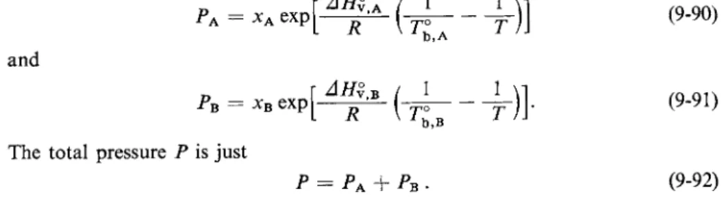
The material of Section 9-2 is now extended to show the various types of boiling point diagrams that one finds for a solution of two volatile liquids. It is first necessary to consider how the total vapor pressure of the solution should vary with composition and temperature. This is most easily done for the case of an ideal solution, for which the two partial pressures are, from Eq. (9-89),
and
r A m Β / 1 PB = xB e x p j ^ —γ — [~ψο The total pressure Ρ is just
b,B
•η-
P = PA + Pb-
(9-90)
(9-91)
(9-92) Substitution of the expressions for PA and PB into Eq. (9-92) gives the equation for the variation of Ρ with composition and temperature.
The general appearance of this function is shown in Fig. 9-14; it is assumed that component A is the one with the lower boiling point.
The upper surface gives the total vapor pressure and the lower one the vapor composition for solutions of a given composition and temperature. The front of the projection corresponds to a cross section at constant temperature, and thus constitutes the vapor pressure-composition diagram for that temperature, as shown in Fig. 9-15(a). The top surface in Fig. 9-14 corresponds to a cross section at constant pressure and therefore to the boiling point diagram for that pressure, as shown in Fig. 9-15(b). Notice that the liquid composition line is now curved and lies below rather than above the vapor composition line.
1 atm
FIG. 9-14. Variation of Ρ with temperature and composition for an ideal solution.
9-7 BOILING POINT DIAGRAMS 325
The normal boiling point diagram is given by a cross section at Ρ = 1 atm.
We can obtain the boiling point versus composition line analytically by setting Ρ = 1 in Eq. (9-92):
1
- '-Η^Ψ- (it ~
+4 ^ (it ~ *)!!·
(9-93) Equation (9-93) reduces to two variables since xA + xB = 1. Since it is trans
cendental, it is best solved by picking successive choices for 7b and solving for corresponding xA or xB . The resulting plot is shown in Fig. 9-15(b). The vapor line gives the compositions of vapor in equilibrium with boiling solutions and is calculated from the corresponding PA and PB values:
(9-94)
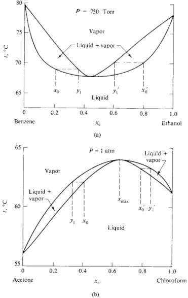
The boiling point diagram is again a phase map. Referring to 9-15(b), we see that if a system of composition x0 is contained in a cylinder with a piston arranged so that the pressure is always 1 atm, the system consists entirely of vapor if Τ > Tx. On cooling to Tx, liquid of composition x1 begins to condense out and by temperature T2 the system consists of liquid of composition x2 and vapor of composition y2. The relative amounts are given on application of the lever principle to the tie-line at T2. At Γ3 the last vapor, of composition v3, has condensed, and below Γ3 the system is entirely liquid.
Figure 9-15 illustrates another point, namely, that the boiling point diagram is (roughly) similar in appearance to that of the vapor pressure diagram turned upside down: The higher vapor pressure liquid is the lower boiling one, and the relative positions of the phase regions are reversed. A similar situation holds for nonideal systems as shown in Fig. 9-16. Positive deviation, leading to a maximum in the vapor pressure diagram, will usually give a minimum boiling system as in Fig.
0 0.2 0.4 0.6 0.8 1.0
Acetone xc Chloroform
(b)
FIG. 9-16. Vapor pressure and boiling point diagrams: (a) Positive deviation from Raoult's law, giving a minimum boiling diagram, (b) Negative deviation from Raoult's law, giving a maximum boiling diagram.
9-7 BOILING POINT DIAGRAMS 327
9-16(a), whereas a negatively deviating system with a minimum in the vapor pressure diagram usually shows maximum boiling behavior, as in Fig. 9-16(b).
Compare with Figs. 9-7 and 9-3.
B. Distillation
If a boiling system is arranged so that the vapors are continuously removed rather than being contained as in the cylinder and piston arrangement, a somewhat different sequence of events occurs. Referring to the case of Fig. 9-15(b), we see that liquid of composition xQ would first boil at T3, producing vapor of compo
sition y3. Since the vapor is richer in A than is the liquid, and is steadily being removed, the liquid composition progressively becomes richer in B, passing compositions x2 a nd Xi, respectively. Unlike the situation with the closed system, however, liquid remains when Tx is reached. This is because the overall vapor composition is not x0 , but rather the average of the compositions of the succession of vapors produced, ranging from y3 to x0. For example, this average vapor composition might be about equal to y2, in which case the relative amount of liquid remaining would be given by the lever (y2 — x0)l(y2 — Xi), or about 50%.
Continued boiling would continue to shift the liquid composition to the right, and the last drop of liquid remaining would be essentially pure B.
A similar analysis applies to Fig. 9-16(a). Liquids of composition either x0 or x0' produce initial vapors of composition yx o r j / j i n both cases the vapor composition is closer to the minimum boiling composition than is the liquid composition. As a a consequence, continued boiling of system JC0 moves the liquid composition progressively toward pure benzene, and continued boiling of system x0' moves it toward pure ethanol. If there is a maximum boiling point, the vapor compositions lie away from the maximum, as compared to the liquid composition, as shown in Fig. 9-16(b). The result is that continued boiling of either liquid x0 or x0' eventually produces liquid of composition xm ax , the maximum boiling composition. At this point the liquid and vapor compositions are the same and continued boiling produces no further change. The system now behaves as though it were a pure liquid and is called an azeotropic mixture. The value of xm ax depends on the pres
sure; Fig. 9-16(b) is, after all, merely one particular isobaric cross section of a general diagram of the type shown in Fig. 9-16. It is possible, however, to use this maximum boiling feature as a means of preparing a standard solution. An example is the hydrochloric acid-water system, for which the maximum boiling composition is 20.222 % HC1 at 760 Torr (but shifts to 20.360 % HC1 at 700 Torr). The standard
ization procedure consists simply in boiling a solution until no further change in boiling point occurs and recording the concentration appropriate to the ambient or barometric pressure.
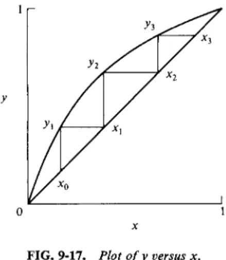
Fractional distillation comprises a series of evaporation-condensation steps.
It is helpful at this point to refer to a diagram of the type shown in Fig. 9-17, in which vapor composition y is plotted against liquid composition x. The case illustrated is that of a relatively ideal solution. Liquid of composition x0 produces some vapor of composition yx. If this vapor is condensed, the effect is to locate a new liquid composition xx on the diagonal. Liquid xx produces vapor y2 and on its condensation, liquid x2 results. The series of steps gives the number of operations needed to reach the final liquid composition xz. This analysis assumes that only a small amount of each liquid is vaporized; in actual practice the fraction is appreciable and so the vapor compositions are always less enriched in the more
FIG. 9-17. Plot of y versus x.
volatile component than in the ideal situation. The detailed treatment of fractional distillation constitutes a major subject in chemical engineering and is beyond the scope of this text.
A special case in distillation is that of two immiscible liquids. A mixture of two such liquids will boil when their combined vapor pressure reaches 1 atm. We thus write the separate Clausius-Clapeyron equations for each pure liquid:
The normal boiling point of the mixture of liquid phases is given by
1
- (it ~ # 1
+" *)]· <
w>
since we require that PA° + PB° = 1. The situation is illustrated in Fig. 9-18.
Boiling of such a mixture produces vapor of composition
= ρ
o
PZ
P Ο= PB°( if P = 1), (9-98)where PA° and PB° are the vapor pressures of the pure liquids at 7b . On continued boiling, one or the other liquid phase will eventually disappear and the boiling point will then revert to that of the remaining liquid.
A procedure of this type is often known as a steam distillation, since a frequent application is the distillation of a mixture of water and an insoluble organic liquid or oil. The advantage is that the oil is thereby distilled at a much lower temperature than would otherwise be needed and with less danger of decomposition. It is also possible to obtain the molecular weight of the oil from Eq. (9-98). If component
9-8 PARTIAL MISCIBILITY 329
A is water, then PA° is given by the measured 7b and PB° is then the ambient or barometric pressure minus PA° and yB is given by Eq. (9-98). With^B and the weight fraction of the distillate known, MB can be calculated.
As an example, suppose that a mixture of an insoluble organic liquid and water boiled at 90.2°C under a pressure of 740.2 Torr. The vapor pressure of pure water is 530.1 Torr at this temperature. The condensed distillate is 71 % by weight of the oil. Evidently PB° is 740.2 — 530.1 or 210.1 Torr; therefore yB = 210.1/740.2 = 0.2838. Since
WB\MB
(WB/MB) + (WA/MAY
where W denotes weight of substance, or
WB _ yB WA
MB 1 - yBMA
then, per 100 g of distillate,
WB 0.2838 29 MB 0.716218.02 and M2 = 71/0.638 111.2 g mole"1.
0.638
9-8 Partial Miscibility
The equilibrium between a liquid solution and a pure solid phase of one of the components is treated in Chapter 10 and that between liquid and solid solutions in Chapter 11. There remains the case of two partially miscible liquid phases. If liquid phases α and β are in equilibrium, then if the system is one of two compo-
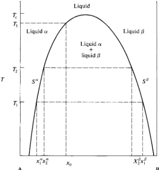
Figure 9-19 shows a schematic temperature-composition plot for two liquids A and B. The left-hand line gives the variation with temperature of Sa and the right- hand line the variation of S*. The behavior illustrated is the very common one in which both solubilities increase with increasing temperature. There is therefore a temperature Tc at which they have become equal and above which the two liquids are completely miscible. The temperature Tc is known as a consolute temperature, in this case, an upper consolute temperature. The figure again has the properties of a phase map. Systems whose overall composition and temperature locate a point in the region between the Sa and S® lines, such as system x0 at Tx, will consist of nents A and B, the condition for equilibrium is that
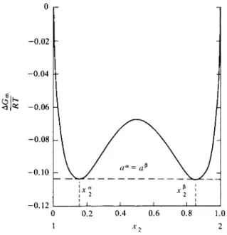
μΑ« = μΑ* and μΒ" = μΒ*. (9-99) As discussed in the Special Topics section, this means that a plot of the molar
free energy of the solution, G/(nA + nB), versus composition shows a double mini
mum, and therefore so, too, does a plot of AGmix versus composition.
The situation is one in which there is a limited solubility of Β in A, giving A-rich solutions designated as α phase, and a limited solubility of A in B, giving B-rich solutions designated as β phase. The maximum solubilities may then be designated as Sa and Ξβ, where Sa is the composition of a solution saturated with respect to Β and Ξβ is that of a solution saturated with respect to A. The compositions Sa and S0 are not very dependent on pressure; quite large pressures are needed to change the free energies of liquids appreciably. They are temperature-dependent, however, and this dependence is customarily shown in plots of solubility versus temperature at 1 atm pressure.