Thermodynamics of mixing methanol with supercritical CO

Thermodynamics of mixing methanol with supercritical CO

2

as seen from computer simulation and

thermodynamic integration

Réka A. Horváth,

¹

George Horvai,

¹

Abdenacer Idrissi,

²

and Pál Jedlovszky,

^3,*

1

Department of Inorganic and Analytical Chemistry, Budapest University of Technology and Economics, Szt. Gellért tér 4, H-1111 Budapest, Hungary

2

University of Lille, Faculty of Sciences and Technologies, LASIR (UMR CNRS 8516), 59655 Villeneuve d’Ascq, France

3

Department of Chemistry, Eszterházy Károly University, Leányka u. 6, H-3300 Eger, Hungary

Running title: Thermodynamics of Mixing Methanol and CO2

*Electronic mail: jedlovszky.pal@uni-eszterhazy.hu (PJ)

Graphical and textual abstract for the contents page:

Thermodynamics of mixing supercritical CO2 with liquid methanol is studied by computer simulation and thermodynamic integration

0

RT/2

A mix

CO2

MeOH

Abstract

The changes of extensive thermodynamic quantities, such as volume, energy, Helmholtz free energy and entropy, occurring upon mixing liquid methanol with supercritical CO2 are calculated by Monte Carlo simulation and thermodynamic integration for all eight combinations of four methanol and two CO2 potential models in the entire composition range at 313 K. The obtained results are also compared with experimental data whenever possible.

The transition of the system from liquid to supercritical state is found to occur at this temperature around the CO2 mole fraction value of 0.95 with all model combinations considered. This liquid to supercritical transition is always accompanied by positive Helmholtz free energy of mixing values and, consequently, by the non-miscibility of the two components. Further, both this non-miscibility around the liquid to supercritical transition and also the miscibility of the two components below this transition, in the liquid regime, are found to be primarily of energetic rather than entropic origin; the entropy of mixing turns out to be very close to zero, and around the liquid to supercritical transition even its qualitative behaviour is strongly model dependent. Finally, it is found that the methanol expansion coefficient is insensitive to the details of the potential models, and it is always in an excellent agreement with experimental data. On the other hand, both the volume and the energy of mixing depend strongly on the molar volume of neat CO2 in the model being used, and in this respect the TraPPE model of CO2 [J. J. Potoff and J. I. Siepmann, AIChE J. 2001, 47, 1676]

performs considerably better than that of Zhang and Duan [Z. Zhang and Z. Duan, J. Chem.

Phys. 2005, 122, 214507].

1. Introduction

In the past decades, supercritical fluids have been increasingly used to replace conventional, toxic organic solvents in a number of processes from nanotechnology to catalysis and from polymer technology to the environmentally friendly destruction of hazardous wastes. [!1-8]

Among the possible supercritical fluids, the most widely used solvent is clearly supercritical CO2 (scCO2) due to its natural abundance, not very high critical temperature, chemical inertness and non-flammability, non-toxicity, and low cost. The solvation ability of scCO2 can substantially be improved by adding other, co-solvent molecules to it. The physical and chemical properties of such mixtures, often referred to as CO2-expanded liquids, [!9] can then be fine tuned by changing, besides the temperature and pressure, also the composition of the system. Further, the chemical character of such solvents can also be altered by the choice of the co-solvent molecule, e.g., by adding a weak base or a hydrogen bonding liquid to the non H-bonding, weak acid, CO2. In this respect, the use of methanol as a co-solvent is of particular importance.

Mixtures of scCO2 and methanol have been intensively studied in the past decades in various respects, focusing on the properties of the one-phase mixture, [!10-14] including its solvation properties concerning various solutes, [!15-18] vapour-liquid equilibrium, [!19-35]

composition dependence of the critical point, [!21,25,26,29,36,37] or multicomponent mixtures including other co-solvents. [!19,20,26,38-40] These experimental studies have also been accompanied by a number of theoretical [!13,20,41-43] and computer simulation [!17,31,44-50] investigations. However, in spite of the large number of studies concerning the thermodynamic properties of this system, very little is known about the change of the thermodynamic quantities occurring upon mixing the two neat components. More precisely, while the expansion coefficient of the co-solvent by scCO2 has been determined at various thermodynamic states, [!21,28,30,31,35] we are not aware of any study concerning the change of the energy, entropy, enthalpy, or Helmholtz free energy accompanying the mixing of the two components, although these quantities could provide a deeper insight into the thermodynamic background, including the nature of the driving force that governs the mixing of these molecules.

The thermodynamics of mixing can be conveniently investigated by computer simulation methods, [!51] in which the appropriately chosen model of the system of interest is

seen at atomistic resolution, and hence the properties of this model system can be accessed in such a detail what cannot be offered by any experimental method. On the other hand, the validity of the model used needs to be tested against existing experimental data. In calculations targeting the thermodynamics of mixing two components, computer simulation methods are accompanied by thermodynamic integration (TI), [!52,53] performed along a fictitious path, in which the neat components are mixed in the ideal gas state, and the mixture is brought back to the thermodynamic state of interest. [!54] This combination of computer simulation and TI has been used to calculate the thermodynamics of mixing of various compounds, [!54-60] including also scCO2 [!56] in the past ten years. It should be noted that such calculations not only offer a deep insight into the nature of the mixture of interest at the molecular level, but the comparison of the results with existing experimental data also provides a stringent test of the validity of not only the potential models used in the simulations, but also that of their compatibility with each other. [!55,57]

In this paper, we investigate the thermodynamics of mixing liquid methanol with scCO2 by Monte Carlo simulation and thermodynamic integration in the entire composition range along the liquid-vapour coexistence line at 313 K. Besides the volume of mixing and expansion coefficient, calculated on the basis of constant pressure simulations, we also determine the energy, entropy, and Helmholtz free energy of mixing by constant volume simulations combined with TI. The calculations are repeated with all possible combinations of two potential models of CO2 and four models of methanol. The various model combinations are assessed by comparing the calculated volumetric properties with existing experimental data.

The paper is organized as follows. In sec. 2, a description of the methods used and details of the calculations performed are given. Thus, besides explaining the calculation of the quantities of mixing along the chosen fictitious thermodynamic path and also the basic principles of the TI method, here we provide also a description of the potential models considered and details of the Monte Carlo simulations and thermodynamic integrations performed. The obtained results are presented and discussed in detail in sec. 3. Finally, in sec.

4, the main conclusions of this study are summarized.

2. Methods

2.1. Calculating the change of thermodynamic quantities upon mixing

The change of the volume (V) and internal energy (U) of mixing can simply be calculated as

2 2 1 1 12

mix V xV x V

V    (1)

and

2 2 1 1 12

mix U xU x U

U    , (2)

where the indices 1, 2, and 12 stand for the neat components 1 and 2, and for their mixture, respectively, while x1 and x2 are the mole fractions of the respective components (for binary mixtures being x1 + x2 = 1). In calculating Vmix, the (molar) volume of the neat components and the mixture can simply be obtained by performing computer simulations of the respective systems on the isothermal-isobaric (N,p,T) ensemble at the temperature and pressure corresponding to the thermodynamic state of interest. Having the molar volumes (and, hence, also the densities) of the neat components and the mixture calculated, the expansion coefficient of component 1, 1, can be evaluated as

 

2 2 12

2 2 1 0 1 1 1

M x

M x M x



   ^ , (3)

where M1 and M2 are the molar mass of the respective neat components, while ₁⁰ and ₁₂ stand for the density of the neat component 1 at atmospheric pressure and that of the mixture at the pressure of interest, respectively.[!35] On the other hand, in calculating Umix, the internal energy of the neat components and the mixture can be obtained by performing simulations on the canonical (N,V,T) ensemble, using the volume obtained from the previous¸

(N,p,T) ensemble simulation.

The change of the Helmholtz free energy, A, occurring upon mixing the neat components 1 and 2, can be calculated as

A_mix A₁₂x₁A₁x₂A₂RT



x₁lnx₁x₂lnx₂



, (4) where A1, A2, and A12 denote the excess Helmholtz free energy of the corresponding systems (with respect to the ideal gas state), while R and T are the gas constant and temperature, respectively. This equation can be associated with the following fictitious thermodynamic path. In the first step, the neat components are brought, in an isochoric way, to the ideal gas state; this step is accompanied by the free energy change (-x1A1 – x2A2). Then, the neat components are mixed in the ideal gas state, accompanied by the free energy change corresponding to the ideal mixing of RT(x1lnx1 + x2lnx2). Finally, the mixture is brought

isochorically back to the thermodynamic state of interest, while the free energy changes by A12. This fictitious thermodynamic path is illustrated in Figure 1 of Ref. [!60]. To calculate the value of Amix by eq. 3, the quantities A1, A2, and A12 need to be evaluated, which can be done by the method of thermodynamic integration, as explained in the following sub-section.

Finally, having Amix and Umix already calculated, the entropy of mixing can simply be given as

T A S_mix U^mix  ^mix

 . (5)

2.2. Thermodynamic integration

The calculation of the Helmholtz free energy in a computer simulation is a far more demanding task than that of the internal energy, because it is proportional to the configurational part of the total canonical partition function (often referred to as the configurational integral), Q, and hence its evaluation requires sampling the entire configurational space rather than only its lowest energy domains. In practice, instead of the total free energy of a given state, usually only the free energy difference between this state of interest, Y, and a suitably chosen reference state, X, is accessible in a computer simulation. In the method of TI, [!52,53] this free energy difference is calculated as an integral along a (fictitious) path connecting the two states, i.e.,

 

) d

1 (

0 X

Y^{ }



^_^_ ^_^



 A

A A

A , (6)

where  is the coupling parameter that defines the path in such a way that its value is 0 and 1 in the reference state, X, and in the state of interest, Y, respectively. Considering the fundamental relations in statistical mechanics between A, Q, and U, i.e.,

Q T k

A _B ln (7)

and

^Q



^exp



^U/kBT



^{, (8)}

the integrand of eq. 6 can be rewritten as

 









 















 



 



 









 

 

 







_{( )}

d )) ( exp(

d )) ( ) exp(

( )

( ) ( )

( _B U

U U U

Q Q

T k A

N N

q q

. (9)

In these equations, kB stands for the Boltzmann constant, =1/kBT, q^N represents the spatial coordinates of all the N particles in the system, and the brackets <…> denote ensemble averaging at a given  value.

To evaluate the ensemble average in eq. 9, first the path connecting states X and Y or, in other words, the continuous function U() needs to be chosen. The conventional choice for this path is a fourth order polynomial, i.e.,

4 X 4 Y (1 ) )

( U U

U     , (10)

where UX and UY stand for the internal energies of the corresponding states. The choice of the fourth power is dictated by the fact that in systems of pairwise additive energy, where the leading term of the potential function decays with r^-12, the use of an exponent smaller than 4 in eq. 10 leads to a singularity (i.e., divergence of U()) at the  = 0 point. [!52] In cases when the Helmholtz free energy difference between the (isochoric) liquid and ideal gas states of a system is calculated, [!61-65] such as in the present study, the reference state X corresponds to the ideal gas, and hence UX ≡ 0. As a consequence, in such cases, eq. 10 simplifies to U() = ⁴UY, and thus, considering also eq. 9, eq. 6 can be rewritten as

  





d 4

) d

( ¹

0 1 3

0





^_^_ ^_^{ }



 A U_Y

A . (11)

It should be recalled that the ensemble averaging in eq. 11 needs to be done at a given value of , which can be done by performing a computer simulation with the potential function U(), as defined in eq. 10. However, considering that, in the present case, U() = ⁴UY, the Boltzmann factor in eq. 9, which is evaluated in each step of a Monte Carlo simulation, can be rewritten as

  

4 Y B

 

Y B ^*



B exp / exp /

/ ) (

exp U  k T   U k T  U k T , (12)

where T^* = T/⁴. In other words, technically the simulation performed at the temperature T with the potential U() is equivalent with that performed at the virtual temperature T^* using the full potential UY. In other words, instead of scaling down the interactions to zero, the ideal

gas state is approached by scaling up the temperature (and thus the kinetic energy of the particles) to infinity. It should again be emphasized that the chosen path connecting the state of interest, Y, and the ideal gas reference state, X, is fictitious, and hence the states along this path, corresponding to the T < T^* <  range of virtual temperatures, have no physical relevance themselves.

The integrand of eq. 11 has been evaluated by performing Monte Carlo simulations at six different  values, namely 0.046911, 0.230765, 0.5, 0.769235, 0.953089, and 1. The first five of these values correspond to the 5-point Gaussian quadrature, [!66] while simulation in

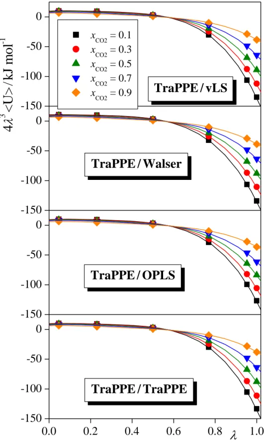
 = 1 has been performed in order to evaluate also the internal energy of the system. In order to perform the integral of eq. 11, a fourth order polynomial has been fitted to the obtained 4³<UY> vs.  data points, and the fitted polynomial has been integrated analytically. The calculated data points along with the fitted polynomials are shown in Figure 1 as obtained at the xCO2 values of 0.1, 0.3, 0.5, 0.7, and 0.9 from the simulations performed with the TraPPE model of CO2 in combination with all four methanol models considered.

2.3. Potential models

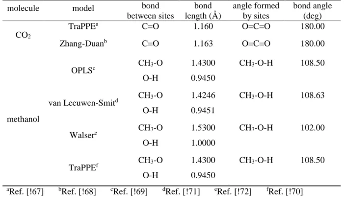
In this study, we consider two potential models of CO2, namely the model belonging to the TraPPE force field [!67] and the one proposed by Zhang and Duan (referred to here as ZD), [!68] and four models of methanol, including the potentials belonging to the OPLS [!69] and TraPPE [!70] force fields and the ones developed by van Leeuwen and Smit (referred to here as vLS) [!71] and by Walser et al. (referred to as Walser). [!72] All of these potential models are rigid, and the CH3 group of methanol is always treated as a united atom. The bond lengths and bond angles corresponding to these models are summarized in Table 1.

All models considered here describe the interaction energy of a molecule pair by the sum of the Lennard-Jones and charge-charge Coulomb interactions acting between all pairs of their sites (i.e., atoms or united atoms). Further, the total energy of the systems is calculated as the sum of the interaction energies of all molecule pairs, thus

   

      







































 ^N 

i

n

j i j

i j

i N

i j

i nj

r q q r

U r

1 1 1 0 ,

6

, 12

1 , 4

4 1

   















  



  . (13)

In this equation, indices i and j run over the molecules in the system,  and  run over all ni

and nj interaction sites of molecules i and j, respectively, N is the total number of molecules,

 and  are the Lennard-Jones distance and energy parameters, respectively, corresponding to the pair of sites  and , related to the parameters corresponding to the individual sites through the Lorentz-Berthelot combination rule: [!51]

2



  

  ^ (14)

and





  

  , (15)

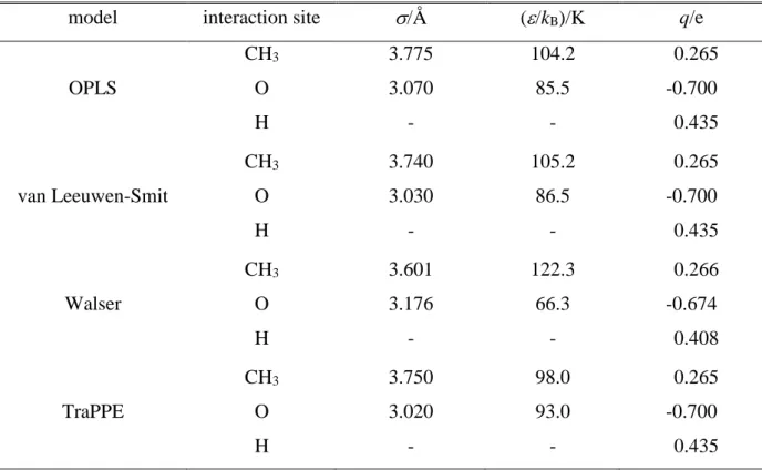
ri,j is the distance between site  of molecule i and site  of molecule j, 0 is the vacuum permittivity, while q and q are the fractional charges carried by the corresponding sites. The interaction parameters , , and q corresponding to the CO2 and methanol models considered are summarized in Tables 2 and 3, respectively.

2.4. Monte Carlo simulations

Monte Carlo simulations of methanol-CO2 mixtures of 12 different compositions, including the two neat systems, have been performed both on the isothermal-isobaric (N,p,T) and canonical (N,V,T) ensemble. The systems simulated have corresponded to the CO2 mole fraction (xCO2) values of 0, 0.1, 0.2, 0.3, 0.4, 0.5, 0.6, 0.7, 0.8, 0.9, 0.95, and 1; the cubic simulation box has always consisted of 500 molecules (see Table 4). Standard periodic boundary conditions have been applied in all simulations. The (N,p,T) ensemble simulations have been performed at the temperature of 313 K and at the pressure corresponding to the experimental vapour-liquid coexistence [!35] of the simulated temperature and composition;

these pressure values are included in Table 4. The choice of the simulation temperature of 313 K has been dictated by the wealth of experimental data available at this temperature, including data used as input of the simulations. [!11,35] The (N,V,T) ensemble simulations have been performed at 313 K (to evaluate Umix), and also at the five virtual temperatures corresponding to the  values of the 5-point Gaussian quadrature (see sec. 2.2.), to evaluate Amix. In these simulations, the volume of the cubic basic simulation box has been set to the equilibrium volume resulted from the corresponding (N,p,T) ensemble simulation.

Simulations have been repeated with all the eight combinations of the two CO2 and four methanol models considered (see sec. 2.3), thus, a total number of more than 600

simulations have been performed in this study. All interactions have been truncated to zero beyond the centre-centre cut-off distance of 12.5 Å, considering the C atom of CO2 and O atom of methanol as the molecular centres. The long range part of the electrostatic interaction has been accounted for by means of the reaction field correction method, [!51,74,75] using the experimental value of the dielectric constant [!11] (see Table 4) in each system.

Simulations have been performed by the program MMC. [!76] In a Monte Carlo step, a randomly chosen molecule has been attempted to be randomly translated by a distance no more than 0.25 Å and randomly rotated around a randomly chosen space-fixed axis by an angle no more than 10^o. In the case of the (N,p,T) ensemble simulations, every 500 particle displacement steps have been followed by a volume change attempt by no more than 150 ų. All moves have been accepted or rejected according to the standard Monte Carlo acceptance criteria. [!51] The ratio of the successful and attempted particle displacement and volume change moves have both been about 0.5. (N,p,T) ensemble simulations have been started from random arrangement of the molecules; (N,V,T) ensemble simulations at 313 K have been started from equilibrium configurations resulted from the preceding (N,p,T) runs, while (N,V,T) simulations at the five virtual temperatures have been started from the final configuration of the run at the previous temperature. In the (N,p,T) ensemble simulations, the systems have been equilibrated for 10⁸-10⁹ Monte Carlo steps, until the volume of the system has fluctuated around its equilibrium value. The volume of the system have been averaged over a subsequent, 10⁸ Monte Carlo steps long equilibrium trajectory. In the case of the (N,V,T) ensemble runs, the equilibration trajectory has been 5 × 10⁷ Monte Carlo steps long, and the energy of the system has been equilibrated in the subsequent, 10⁸ Monte Carlo steps long run in every case. Equilibrium snapshots of the systems corresponding to the xCO2 values of 0.3, 0.7, and 0.95 are shown in Figure 2, as taken out from the (N,V,T) ensemble simulations performed at 313 K with the ZD model of CO2 and vLS model of methanol.

3. Results and discussion

3.1. Volumetric results

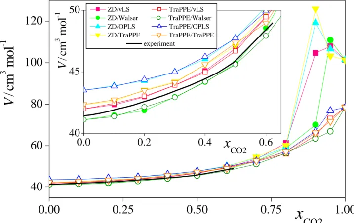
The composition dependence of the molar volume and volume of mixing of the eight model combinations of methanol and CO2 considered are plotted in Figure 3 and Figure 4, respectively, as resulted from the simulations. As is seen, the molar volume of the system increases with increasing CO2 mole fraction up to xCO2 = 0.8 in every case, reflecting the

gradual expansion of methanol by CO2. However, between the xCO2 values of 0.8 and 1, the systems described by different model combinations behave in noticeably different ways.

Thus, when CO2 is described by the ZD model, V always goes through a marked maximum in the xCO2 range of 0.9-0.95. Similar behaviour was observed earlier in the simulations of ethanol-CO2 and acetone-CO2 mixtures. [!56] The occurrence of this peak is related to the fact that the mixture of liquid methanol and scCO2, being in the liquid phase up to rather high CO2

mole fractions, becomes supercritical in this composition range at the temperature of the simulations, [!77] but methanol molecules still try to form a liquid droplet in the supercritical medium (see the rightmost panel of Fig. 2). On the other hand, in all cases corresponding to the TraPPE model of CO2, the obtained V(xCO2) curve is always monotonous, although its slope between the xCO2 values of 0.9 and 1 depends strongly on the methanol model used. It should be emphasized, however, that the fact that we have not found any peak of the V(xCO2) curve here does not necessarily mean that no such peak exists. Since this peak is rather narrow, its width being comparable with the composition resolution used in this study, it might well be the case that a narrow such peak is located either between the xCO2 values of 0.9 and 0.95, or between 0.95 and 1, i.e., in a sufficiently narrow composition range that has not been explored in the present study.

Nevertheless, the model combinations involving the ZD and the TraPPE models of CO2 have clearly showed different volumetric behaviour in mixtures of low methanol content.

Although experimental data are scarce in this composition range, the comparison of the molar volume of neat CO2 with the experimental value is decisive in this respect. Thus, while the molar volume obtained for the ZD model of CO2 at 313 K of 101.3 cm³/mol overestimates the experimental value of 67.2 cm³/mol [!78] by almost 50%, the molar volume of the TraPPE model of 78.5 cm³/mol agrees with this value within about 15%. Similar failure of the ZD model in predicting the pressure and density of neat CO2 was pointed out earlier by Merker et al. [!79] It should also be noted that the molar volume of scCO2 depends rather sensitively on the temperature, thus, at the simulation pressure of neat CO2 of 105.1 bar a temperature shift of 1 K leads to an about 2 cm³/mol change in the molar volume. Thus, the 11.3 cm³/mol deviation of the molar volume of the TraPPE model with respect to the experimental value corresponds to only an about 5-6 K temperature shift.

The inset of Fig. 3 shows the comparison of the obtained molar volumes with the experimental data of Aida et al [!35] in the composition range of this experimental data set, i.e., up to the xCO2 value of about 0.6, on an enlarged scale. Not surprisingly, in this low xCO2

range, the obtained results do not depend noticeably on the CO2 model chosen. Among the

methanol models considered, that of Walser et al. gives a slightly better, while OPLS a clearly worse reproduction of the experimental data in this respect than the other ones.

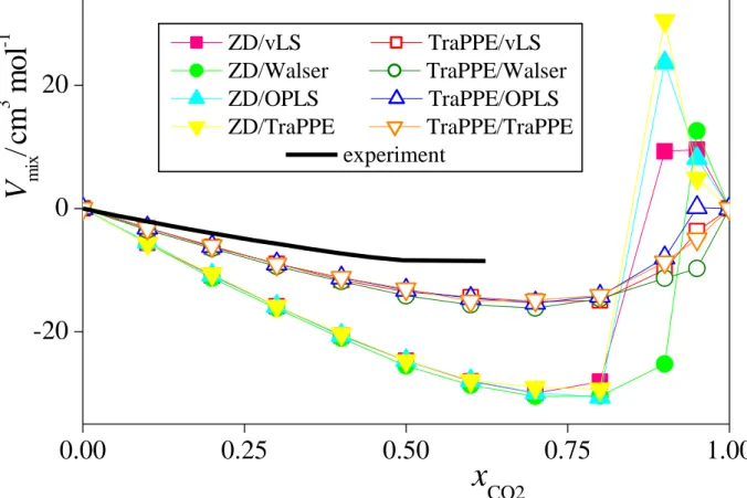
The differences between the obtained volumes of mixing data (Fig. 4) reflect primarily the difference in the molar volume of neat CO2 as obtained with the ZD and TraPPE models.

Thus, the Vmix(xCO2) curves corresponding to the same CO2 model are rather similar to each other up to xCO2 = 0.8, those corresponding to the ZD model giving consistently lower Vmix

values (as the molar volume of neat CO2, weighted with xCO2 in the mixture, is subtracted when calculating Vmix, see eq. 1), while those corresponding to the TraPPE model of CO2

being in a much better agreement with the experimental curve. Further, between the xCO2

values of 0.8 and 1, the Vmix(xCO2) curves corresponding to all model combinations involving the ZD potential of CO2 turn to positive values and go through a clear maximum, reflecting the large molar volume of these mixtures. No such maximum is seen, however, when the TraPPE model of CO2 is considered, except for the tiny peak of the TraPPE/OPLS model combination at xCO2 = 0.95.

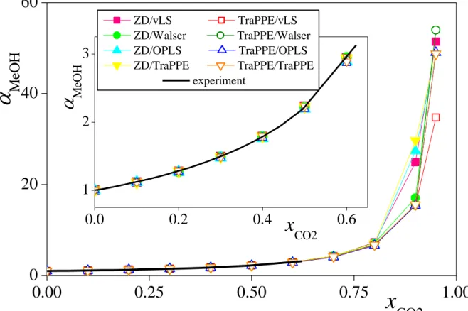
Finally, we have also calculated the expansion coefficient of liquid methanol, MeOH

(see eq. 3), for the eight model combinations considered. The obtained results are shown and compared with experimental data [!35] in Figure 5. As it is seen, the value of the expansion coefficient is rather insensitive to the details of the potential models. This is not surprising, since the expansion coefficient does not depend on the molar volume (or density) of neat CO2

(see eq. 3), the only quantity the value of which has turned out to be strongly model dependent. Thus, the results obtained with all the eight model combinations considered are almost indistinguishable from each other up to xCO2 = 0.8, being also in a perfect agreement with the experimental data in the entire range of their existence (see the inset of Fig. 5). At xCO2 > 0.8, different model combinations behave in different ways in this respect (although all of them result in a monotonously increasing curve), reflecting again the large differences in their molar volumes in this composition range, and, ultimately, the difference between the molar volumes of the ZD and TraPPE models of CO2.

3.2. Energetic results

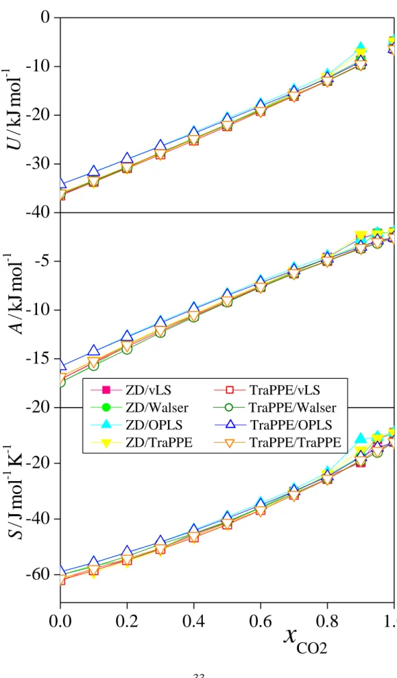
The composition dependence of the molar energy, Helmholtz free energy and entropy of the eight model combinations of methanol and CO2 considered are shown in Figure 6, while the corresponding energies, Helmholtz free energies and entropies of mixing are plotted in Figure 7, as obtained from the simulations. As is seen, the energy of the system increases almost linearly with xCO2, suggesting that the mixing of the two components, from the energetic point

of view, is close to ideal. The molar Helmholtz free energy and entropy also increase steadily with xCO2, although the A(xCO2) and S(xCO2) curves noticeably deviate from the linear shape.

When the TraPPE model of CO2 is considered, the shapes of all these three curves change smoothly in the entire composition range, while in the case of the ZD model they all exhibit a little hump in the xCO2 range of 0.9-0.95, reflecting the anomalously low density of these systems in this composition range (see Fig. 3). It is also seen that, at low CO2 mole fractions, the OPLS model of methanol corresponds to noticeably higher energy and free energy values of the mixtures than the other three methanol models considered. This difference probably cannot simply be explained by the 2-6% lower density of the systems involving the OPLS methanol model than that of the others (as similar density differences corresponding to the Walser and vLS or TraPPE methanol models are not reflected in the U and A values) . Instead, it might well be the consequence of some inaccuracies in the parameterization of OPLS, a model developed 1-1.5 decades earlier than the other ones considered here, which are likely related to the neglect of the long range part of the electrostatic interaction in the parameterization procedure. [!69]

The free energy of mixing of the eight model combinations behave rather similarly to each other in the entire composition range. Thus, apart from its peak at xCO2 = 0.95, its value is always negative, reflecting the miscibility of methanol with CO2 under these thermodynamic conditions. However, at xCO2 = 0.95, i.e., around the liquid to supercritical transition of the mixture, this miscibility is no longer preserved, methanol is separated from scCO2 and forms clusters of liquid-like density (see the right panel of Fig. 2), such as in the case of ethanol-CO2 and acetone-CO2 mixtures. [!56] It should also be noted that the thermodynamic driving force of the miscibility of the two components up to xCO2 = 0.9 is rather weak, as the Amix(xCO2) curves are always well above the curve corresponding to the ideal mixing (dotted line in Fig. 7), and the value of Amix remains always below RT/2, i.e., the average kinetic energy of the molecules along one degree of freedom. Similarly, the peak of the Amix(xCO2) curves at xCO2 = 0.95 is also considerably smaller than RT/2 in every case, indicating that the thermodynamic driving force of the non-miscibility of the system at this composition is also rather weak.

As is seen from Fig. 7, the Umix(xCO2) curve goes, for all model combinations considered, clearly below zero up to xCO2 = 0.8, reflecting presumably the attractive weak acid – weak base interactions occurring between the CO2 and methanol molecules, and becomes positive (with the exception of the TraPPE/Walser system) at xCO2 = 0.95, where the two components do not mix with each other. It is also seen that the too low density of the ZD

model of CO2, resulting also in too small energy (in magnitude) of neat CO2, amplifies the Umix data corresponding to all model combinations involving this model both below and above zero. On the other hand, the Smix(xCO2) data are rather close to zero in the entire composition range, being even consistently negative for certain model combinations (e.g., ZD/Walser or ZD/TraPPE). Further, Smix is clearly well below the value corresponding to the ideal mixing for all model combinations considered in the entire composition range. The reason for this entropy decrease (with respect to the ideal mixing), besides the orientational restrictions implied by the aforementioned weak acid – weak base interactions, is probably caused by the decrease of the molar volume (see Fig. 4), or increase of the density occurring upon mixing. Interestingly, even the qualitative behaviour of Smix is model dependent at the non-miscibility composition of xCO2 = 0.95. All these findings indicate that both the miscibility of methanol and CO2 up to the xCO2 value of about 0.9 and their non-miscibility around xCO2 = 0.95 are primarily of energetic rather than entropic origin.

4. Summary and conclusions

In this paper we have investigated in detail the changes of several extensive thermodynamic quantities, i.e., volume, energy, Helmholtz free energy, and entropy, occurring upon mixing liquid methanol and supercritical CO2 in different proportions at 313 K on the basis of Monte Carlo computer simulations and thermodynamic integration, considering all eight combinations of four selected methanol and two CO2 potential models. It has turned out that, with increasing mole fraction of CO2, the system enters into the supercritical regime in the xCO2 range of about 0.9-0.95, accompanied by either a clear maximum of the V(xCO2) curve, or, at lest, a change of its smooth slope. We cannot exclude the possibility that a similar maximum of V(xCO2) occurs, between two compositions considered in the present study, even in the case of those model combinations for which our results do not indicate the presence of such a maximum. This anomalous behaviour of the V(xCO2) curve around the liquid to supercritical transition is also reflected in the shape of the U(xCO2), A(xCO2), and S(xCO2) data, and hence also in the corresponding changes of these quantities occurring upon mixing. The Helmholtz free energy of mixing is negative up to the CO2 mole fraction of 0.8 and positive around 0.95 in every case, marking the composition ranges corresponding to the miscibility and non-miscibility, respectively, of the methanol and CO2 molecules. It is also found that the thermodynamic driving force is rather weak in both cases, as the magnitude of Amix remains

always below RT/2, i.e., the average kinetic energy of the molecules along one degree of freedom. Both the miscibility (up to xCO2 ≈ 0.8) and the non-miscibility (at xCO2 ≈ 0.95) of these molecules are found to be primarily of energetic rather than entropic origin, as the entropy of mixing remains close to zero in the entire composition range, and even the qualitative behaviour of the Smix(xCO2) curve, unlike that of Umix(xCO2), is also strongly model dependent.

Concerning the reliability of the various model combinations considered it is found, in accordance with earlier claims, [!56,79] that the ZD model of CO2 strongly overestimates the molar volume (and hence underestimates the density) of neat CO2, whereas the OPLS model of methanol somewhat overestimates the molar volume of the methanol-rich systems, for which it also results in smaller energies (in magnitude) than the other methanol models considered. The remaining three model combinations, i.e., TraPPE/vLS, TraPPE/Walser and TraPPE/TraPPE lead to rather similar results, which are also in good agreement with existing experimental data. Among these three model combinations, TraPPE/Walser reproduces the experimental molar volume of the mixtures somewhat better than the other two in the entire composition range in which it was measured.

Acknowledgements

This work has been supported by the Hungarian NKFIH Foundation under Project Nos.

119732, 120075 and 134596, and by the EFOP project “Complex Development of Research Capacities and Services at the Eszterhazy Karoly University” under project No. EFOP-3.6.1- 16-2016-00001.

References

1 C. A. Eckert, B. L. Knutson and P. G. Debenedetti, Supercritical fluids as solvents for chemical and materials processing, Nature 1996, 383, 313-318.

2 H. J. Bleyl, J. Abeln, N. Boukis, H. Goldacker, M. Kluth, A. Kruse, G. Petrich, H.

Schmieder and G. Wiegand, Hazardous Waste Disposal by Supercritical Fluids, Separation Sci. Technol. 1997, 32, 459-485.

3 J. F. Brennecke and J. E. Chateauneuf, Homogeneous Organic Reactions as Mechanistic Probes in Supercritical Fluids, Chem. Rev. 1999, 99, 433-452.

4 A. Baiker, Supercritical Fluids in Heterogeneous Catalysis, Chem. Rev. 1999, 99, 453- 474.

5 J. L. Kendall, D. A. Canelas, J. L. Young and J. M. DeSimone, Polymerizations in Supercritical Carbon Dioxide, Chem. Rev. 1999, 99, 543-564.

6 C. F. Kirby and M. A. McHugh, Phase Behavior of Polymers in Supercritical Fluid Solvents, Chem. Rev. 1999, 99, 565-602.

7 K. P. Johnston and P. Shah, Making Nanoscale Materials with Supercritical Fluids, Science 2004, 303, 482-

8 H. Weingärtner and E. U. Franck, Supercritical Water As a Solvent, Angew. Chem.

Int. Ed. 2005, 44, 2672-2692.

9 P. G. Jessop and Subramaniam, Gas-Expanded Liquids, Chem. Rev. 2007, 107, 2666- 2694.

10 T. A. Berger and J. F. Deye, Composition and Density Effects Using Methanol/Carbon Dioxide in Packed Column Supercritical Fluid Chromatography, Anal. Chem. 1990, 62, 1181-1185.

11 S. B. Lee, R. L. Smith, H. Inomata and K. Arai, Coaxial probe and apparatus for measuring the dielectric spectra of high pressure liquids and supercritical fluid mixtures. Rev. Sci. Instruments 2000, 71, 4226-4230.

12 M. Maiwald, H. Li, T. Schnabel, K. Braun and H. Hasse, On-line ¹H NMR spectroscopic investigation of hydrogen bonding in supercritical and near critical CO2- methanol up to 35 MPa and 403 K, J. Supercrit. Fluids 2007, 43, 267-275.

13 M. Kariznovi, H. Nourozieh and J. Abedi, Experimental measurements and predictions of density, viscosity, and carbon dioxide solubility in methanol, ethanol, and 1-propanol, J. Chem. Thermodyn. 2013, 57, 408-415.

14 C. Rivas, B. Gimeno, R. Bravo, M. Artal, J. Fernández, S. T. Blanco and M. I.

Velasco, Thermodynamic properties of a CO2 -rich mixture (CO2 + CH3OH) in conditions of interest for carbon dioxide capture and storage technology and other applications. J. Chem. Thermodyn. 2016, 98, 272-281.

15 M. Monserrate and S. V. Olesik, Evaluation of SFE-CO2 and Methanol-CO2 Mixtures for the Extraction of Polynuclear Aromatic Hydrocarbons from House Dust, J.

Cromatogr. Science 1997, 35, 82-90.

16 I. H. Lin and C. S. Tan, Measurement of diffusion coefficients of p- chloronitrobenzene in CO2-expanded methanol, J. Supercrit. Fluids 2008, 46, 112- 117.

17 J. L. Gohres, A. V. Popov, R. Hernandez, C. L. Liotta and C. A. Eckert, Molecular Dynamics Simulations of Solvation and Solvent Reorganization Dynamics in CO2- Expanded Methanol and Acetone, J. Chem. Theor. Comput. 2009, 5, 267-275.

18 M. Banchero, A. Ferri and L. Manna, The phase partition of disperse dyes in the dyeing of polyethylene terephtalate with a supercritical CO2/methanol mixture, J.

Supercrit. Fluids 2009, 48, 72-78.

19 W. Weber, S. Zeck and H. Knapp, Gas solubilities in liquid solvents at high pressures:

apparatus and results for binary and ternary systems of N2, CO2 and CH3OH. Fluid Phase Equil. 1984, 18, 253-278

20 T. Chang and R. W. Rousseau, Solubilities of carbon dioxide in methanol and methanol-water at high pressures: experimental data and modeling. Fluid Phase Equil.

1985, 23, 243-258.

21 E. Brunner, W. Hültenschmidt and G. Schlichthärle, Fluid mixtures at high pressures IV. Isothermal phase equilibria in binary mixtures consisting of (methanol + hydrogen or nitrogen or methane or carbon monoxide or carbon dioxide). J. Chem. Thermodyn.

1987, 19, 273-291.

22 J. H. Hong and R. Kobayashi, Vapor-liquid equilibrium studies for the carbon dioxide- methanol system. Fluid Phase Equil. 1988, 41, 269-276.

23 K. Suzuki, H. Sue, M. Itou, R. L. Smith, H. Inomata, K. Arai and S. Saito, Isothermal Vapor-Liquid Equilibrium Data for Binary Systems at High Pressures: Carbon Dioxide–Methanol, Carbon Dioxide–Ethanol, Carbon Dioxide–1-Propanol, Ethane–

Ethanol, and Ethane–1-Propanol Systems. J. Chem. Eng. Data 1990, 35, 63-66.

24 S. H. Page, S. R. Goates and M. L. Lee, Methanol/CO2 Phase Behavior in Supercritical Fluid Cromatography and Extraction. J. Supercrit. Fluids 1991, 4, 109- 117.

25 A. D. Leu, S. Y. K. Chung and D. B. Robinson, The equilibrium phase properties of (carbon dioxide + methanol). J. Chem. Thermodyn. 1991, 23, 979-985.

26 J. H. Yoon, H. S. Lee and H. Lee, High-Pressure Vapor-Liquid Equilibria for Carbon Dioxide + Methanol, Carbon Dioxide + Ethanol, and Carbon Dioxide + Methanol + Ethanol. J. Chem. Eng. Data 1993, 38, 53-55.

27 T. S. Reighard, S. T. Lee and S. V. Olesik, Determination of methanol/CO2 and acetonitrile/CO2 phase equilibria using a variable-volume view cell. Fluid Phase Equil. 1996, 123, 215-230.

28 C. J. Chang, K. L. Chiu and C. Y. Day, A new apparatus for the determination of P-x- y diagrams and henry’s constants in high pressure alcohols with critical carbon dioxide. J. Supercrit. Fluids 1998, 12, 223-237.

29 S. N. Joung, C. W. Yoo, H. Y. Shin, S. Y. Kim, K. P. Yoo, C. S. Lee and W. S. Huh, Measurements and correlation of high-pressure VLE of binary CO2-alcohol systems (methanol, ethanol, 2-methoxyethanol and 2-ethoxyethanol). Fluid Phase Equil. 2001, 185, 219-230.

30 K. Bezanehtak, G. B. Combes, F. Dehghani, N. R. Foster and D. L. Tomasko, Vapor- Liquid Equilibrium for Binary Systems of Carbon Dioxide + Methanol, Hydrogen + Methanol, and Hydrogen + Carbon Dioxide at High Pressures. J. Chem. Eng. Data 2002, 47, 161-168.

31 Y. Houndonougbo, H. Jin, B. Rajagopalan, K. Wong, K. Kuczera, B. Subramaniam and B. Laird, Phase Equilibria in Carbon Dioxide Expanded Solvents: Experiments and Molecular Simulations. J. Phys. Chem. B 2006, 110, 13195-13202.

32 C. Secuianu, V. Feroiu and D. Geană, Phase Equilibria experiments and calculations for carbon dioxide + methanol binary system. Cent. Eur. J. Chem. 2009, 7, 1-7.

33 K. Tochigi, T. Namae, T. Suga, H. Matsuda, K. Kurihara, M. C. dos Ramos and C.

McCabe, Measurement and prediction of high-pressure vapor-liquid equilibria for binary mixtures of carbon dioxide + n-octane, methanol, ethanol, and perfluorohexane.

J. Supercrit. Fluids 2010, 55, 682-689.

34 Y. Sato, N. Hosaka, K. Yamamoto and H. Inomata, Compact apparatus for rapid measurement of high-pressure phase equilibria of carbon dioxide expanded liquids.

Fluid Phase Equil. 2010, 296, 25-29.

35 T. Aida, T. Aizawa, M. Kanakubo and H. Nanjo, Relation between Volume Expansion and Hydrogen Bond Networks for CO2-Alcohol Mixtures at 40 ^oC. J. Phys. Chem. B 2010, 114, 13628-13636.

36 E. Brunner, Fluid mixtures at high pressures I. Phase separation and critical phenomena of 10 binary mixtures of (a gas + methanol). J. Chem. Thermodyn. 1985, 17, 671-679.

37 J. W. Ziegler, J. G. Dorsey, T. L. Chester and D. P. Innis, Estimation of Liquid-Vapor Critical Loci for CO2-Solvent Mixtures Using Peak-Shape Method. Anal. Chem. 1995, 67, 456-461.

38 K. Suzuki, H. Sue, M. Itou, R. L. Smith, H. Inomata, K. Arai and S. Saito, High Pressure Vapor-Liquid Equilibrium Data of the 10-Component System Hydrogen,

Carbon Monoxide, Carbon Dioxide, Water, Methane, Ethane, Propane, Methanol, Ethanol, and 1-Propanol at 313.4 and 333.4 K. J. Chem. Eng. Data 1990, 35, 67-69.

39 S. T. Lee, T. S. Reighard and S. V. Olesik, Phase diagram studies of methanol-H2O- CO2 and acetonitrile- H2O-CO2 mixtures. Fluid Phase Equilib. 1996, 122, 223-241.

40 G. V. S. M. Carrera, Z. P. Visak, R. M. Lukasik and M. Nunes da Ponte, CO2 + methanol + glycerol: multiphase behaviour, J. Supercrit. Fluids 2018, 141, 260-264.

41 S. G. Cardoso, G. M. N. Costa and S. A. B. Vieira de Melo, Assessment of the liquid mixture density effect on the prediction of supercritical carbon dioxide volume expansion of organic solvents by Peng-Robinson equation of state. Fluid Phase Equilib. 2016, 425, 196-205.

42 M. Khalifa, B. Housam and B. Ahmed, Modeling of the phase behavior of CO2 in water, methanol, ethanol and acetone by different equations of state. Fluid Phase Equilib. 2018, 469, 9-25.

43 S. Abdolbaghi, A. Mohamadnazar, M. Hasanipanah and A. Barati-Harooni, Comparison between a soft computing model and thermodynamic models for prediction of phase equilibria in binary mixtures containing 1-alkanol, n-alkane, and CO2. Fluid Phase Equilib. 2020, 503, 112307-1-22.

44 G. Chatzis and J. Samios, Binary mixtures of supercritical carbon dioxide with methanol. a molecular dynamics simulation study. Chem. Phys. Letters 2003, 374, 187-193.

45 T. Aida and H. Inomata, MD simulation of the self-diffusion coefficient and dielectric properties of expanded liquids — I. Methanol and carbon dioxide mixtures, Mol.

Simul. 2004, 30, 407–412.

46 C. L. Shukla, J. P. Hallett, A. V. Popov, R. Hernandez, C. L. Liotta and C. A. Eckert, Molecular Dynamics Simulation of the Cybotactic Region in Gas-Expanded Methanol-Carbon Dioxide and Acetone-Carbon Dioxide Mixtures. J. Phys. Chem. B 2006, 110, 24101-24111.

47 T. Schnabel, A. Srivastava, J. Vrabec and H. Hasse, Hydrogen Bonding of Methanol in Supercritical CO2: Comparison between ¹H NMR Spectroscopic Data and Molecular Simulation Results. J. Phys. Chem. B 2007, 111, 9871-9878.

48 Houndonougbo, Y. Kuczera, K. Subramaniam, B. Laird, B. Prediction of phase equilibria and transport properties in carbon dioxide expanded solvents by molecular simulation. Mol. Simul. 2007, 33, 861-869.

49 Gohres, J. L. Kitchens, C. L. Hallett, J. P. Popov, A. V. Hernandez, R. Liotta, C. L.

Eckert, C. A. A Spectroscopic and Computational Exploration of the Cybotactic Region of Gas-Expanded Liquids: Methanol and Acetone. J. Phys. Chem. B 2008, 112, 4666-4673.

50 Gurina, D. L. Antipova, M. L. Odintsova, E. G. Petrenko, V. E. Selective solvation in cosolvent-modified supercritical carbon dioxide on the example of hydroxycinnamic acids. The role of cosolvent self-association. J. Supercrit. Fluids 2018, 139, 19-29.

51 M. P. Allen and D. J. Tildesley, Computer Simulation of Liquids, Clarendon Press, Oxford, 1987.

52 M. Mezei and D. L. Beveridge, Free Energy Simulations. Ann. Acad. Sci. N.Y. 1986, 482, 1-23.

53 A. R. Leach, Molecular Modelling, Longman, Singapore, 1996.

54 M. Darvas, P. Jedlovszky and G. Jancsó, Free Energy of Mixing of Pyridine and Its Methyl-Substituted Derivatives with Water, As Seen from Computer Simulations. J.

Phys. Chem. B 2009, 113, 7615-7620.

55 P. Jedlovszky, A. Idrissi and G. Jancsó, Can existing models qualitatively describe the mixing behavior of acetone with water? J. Chem. Phys. 2009, 130, 124516-1-7.

56 A. Idrissi, I. Vyalov, M. Kiselev and P. Jedlovszky, Assessment of the potential models of acetone/CO2 and ethanol/CO2 mixtures by computer simulation and thermodynamic integration in liquid and supercritical states. Phys. Chem. Chem. Phys.

2011, 13, 16272-16281.

57 A. Pinke and P. Jedlovszky, Modeling of Mixing Acetone and Water: How Can Their Full Miscibility Be Reproduced in Computer Simulations? J. Phys. Chem. B 2012, 116, 5977-5984.

58 A. Idrissi, K. Polok, M. Barj, B. Marekha, M. Kiselev and P. Jedlovszky, Free Energy of Mixing of Acetone and Methanol – a Computer Simulation Investigation. J. Phys.

Chem. B 2013, 117, 16157-16164.

59 A. Idrissi, B. Marekha, M. Barj and P. Jedlovszky, Thermodynamics of Mixing Water with Dimethyl Sulfoxide, As Seen from Computer Simulations. J. Phys. Chem. B 2014, 118, 8724-8733.

60 B. Kiss, B. Fábián, A. Idrissi, M. Szőri and P. Jedlovszky, Miscibility and Thermodynamics of Mixing of Different Models of Formamide and Water in Computer Simulation, J. Phys. Chem. B 2017, 121, 7147-7155, erratum: J. Phys.

Chem. B 2017, 121, 9319-9319.

61 M. Mezei, S. Swaminathan and D. L. Beveridge, Ab Initio Calculation of the Free Energy of Liquid Water. J. Am. Chem. Soc. 1978, 100, 3255-3256.

62 M. Mezei, Direct calculation of the excess free energy of the dense lennard-jones fluid Mol. Simul. 1989, 2, 201-207.

63 M. Mezei, Polynomial Path for the Calculation of Liquid State Free Energies from Computer Simulations Tested on Liquid Water. J. Comp. Chem. 1992, 13, 651-656.

64 P. Mináry, P. Jedlovszky, M. Mezei and L. Turi, A Comprehensive Liquid Simulation Study of Neat Formic Acid. J. Phys. Chem. B 2000, 104, 8287-8294..

65 P. Jedlovszky, L. B. Pártay, A. P. Bartók, V. P. Voloshin, N. N. Medvedev, G.

Garberoglio and R. Vallauri, Structural and thermodynamic properties of different phases of supercooled liquid water. J. Chem. Phys. 2008, 128, 244503-1-12.

66 P. J. Davis and I. Polonsky, in Handbook of Mathematical Functions with Formulas, Graphs, and Mathematical Tables, eds. M. Abramowitz and I. A. Stegun, National Bureau of Standards: Washington, D. C., 1972, pp. 875-924.

67 J. J. Potoff and J. I. Siepmann, Vapor-Liquid Equilibria of Mixtures Containing Alkanes, Carbon Dioxide, and Nitrogen. AIChE J. 2001, 47, 1676-1682.

68 Z. Zhang and Z. Duan, An optimized molecular potential for carbon dioxide, J. Chem.

Phys. 2005, 122, 214507-1-15.

69 W. L. Jorgensen, Optimized Intermolecular Potential Functions for Liquid Alcohols. J.

Phys. Chem. 1986, 90, 1276-1284.

70 B. Chen, J. J. Potoff and J. I. Siepmann, Monte Carlo Calculations for Alcohols and Their Mixtures with Alkanes. Transferable Potentials for Phase Equilibria. 5. United- Atom Description of Primary, Secondary, and Tertiary Alcohols. J. Phys. Chem. B 2001, 105, 3093-3104.

71 M. E. van Leeuwen and B. Smit, Molecular Simulation of the Vapor-Liquid Coexistence Curve of Methanol, J. Phys. Chem. 1995, 99, 1831-1833.

72 R. Walser, A. E. Mark, W. F. van Gunsteren, M. Lauterbach and G. Wipff, The effect of force-field parameters on properties of liquids: Parametrization of a simple three- site model for methanol. J. Chem. Phys. 2000, 112, 10450-10459.

73 CRC Handbook of Chemistry and Physics, 44^th Edition, NIST, Washington D. C., 1962-1963.

74 J. A. Barker and R. O. Watts, Monte Carlo studies of the dielectric properties of water- like models. Mol. Phys. 1973, 26, 789-792.

75 M. Neumann, The dielectric constant of water. Computer simulations with the MCY potential. J. Chem. Phys. 1985, 82, 5663-5672.

76 M. Mezei, MMC: Monte Carlo program for simulation of molecular assemblies. URL:

http://inka.mssm.edu/~mezei/mmc (last accessed: 03/03/2020).

77 B. Fábián, G. Horvai, A. Idrissi and P. Jedlovszky, Vapour-liquid equilibrium of acetone-CO2 mixtures of different compositions at the vicinity of the critical point. J.

CO2 Utiliz. 2019, 34, 465-471.

78 NIST Standard Reference Simulation Website, NIST Standard Reference Database Number 173, eds, V. K. Shen, D. W. Siderius, W. P. Krekelberg and H. W. Hatch, NIST, Gaithersburg, http://doi.org/10.18434/T4M88Q (last accessed: 03/03/2020).

79 T. Merker, J. Vrabec and H. Hasse, Comment on “An optimized potential for carbon dioxide” [J. Chem. Phys. 122, 214507 (2005)]. J. Chem. Phys. 2008, 129, 087101.

Tables

Table 1 Geometry parameters of the potential models considered

molecule model bond

between sites

bond length (Å)

angle formed by sites

bond angle (deg) CO2

TraPPE^a C=O 1.160 O=C=O 180.00

Zhang-Duan^b C=O 1.163 O=C=O 180.00

methanol

OPLS^c CH3-O 1.4300 CH3-O-H 108.50

O-H 0.9450

van Leeuwen-Smit^d CH3-O 1.4246 CH3-O-H 108.63

O-H 0.9451

Walser^e CH3-O 1.5300 CH3-O-H 102.00

O-H 1.0000

TraPPE^f CH3-O 1.4300 CH3-O-H 108.50

O-H 0.9450

aRef. [!67] ^bRef. [!68] ^cRef. [!69] ^dRef. [!71] ^eRef. [!72] ^fRef. [!70]

Table 2 Interaction parameters of the CO2 models condsidered

model atom /Å (/kB)/K q/e

TraPPE C 2.800 27.0 0.7000

O 3.050 79.0 -0.3500

Zhang-Duan C 2.792 28.8 0.5888

O 3.000 82.6 -0.2944

Table 3 Interaction parameters of the methanol models condsidered

model interaction site /Å (/kB)/K q/e

CH3 3.775 104.2 0.265

OPLS O 3.070 85.5 -0.700

H - - 0.435

CH3 3.740 105.2 0.265

van Leeuwen-Smit O 3.030 86.5 -0.700

H - - 0.435

CH3 3.601 122.3 0.266

Walser O 3.176 66.3 -0.674

H - - 0.408

CH3 3.750 98.0 0.265

TraPPE O 3.020 93.0 -0.700

H - - 0.435

Table 4 Characteristics of the systems simulated

xCO2 NCO2 Nmethanol p/bar^a ^e

0.0 0 500 0.423^b 28.6

0.1 50 450 18.6 25.2

0.2 100 400 36.2 19.8

0.3 150 350 49.1 14.9

0.4 200 300 60.5 11.0

0.5 250 250 69.9 7.45

0.6 300 200 74.6 4.93

0.7 350 150 78.93 3.92

0.8 400 100 82.9 2.83

0.9 450 50 87.1 2.01

0.95 475 25 95.0^c 1.72

1.0 500 0 105.1^b,d 1.37

aRef. [!35] ^bRef. [!73] ^cExtrapolated using data of Refs. [!35] and [!73] ^dValue along the supercritical extension of the vapour-liquid coexistence curve ^eRef. [!11]

Figure legend

Fig 1 Integrand of the thermodynamic integration (eq. 11), obtained at six  points for the combination of the TraPPE model of CO2 with the vLS (top panel), Walser (second panel), OPLS (third panel), and TraPPE (bottom panel) models of methanol (full symbols), together with the fourth order polynomials fitted to these data (solid curves) at the CO2 mole fraction values of 0.1 (black, squares), 0.3 (red, circles), 0.5 (green, up triangles), 0.7 (blue, down triangles), and 0.9 (orange, diamonds).

Fig. 2 Equilibrium snapshots of the systems corresponding to the CO2 mole fraction values of 0.3 (left), 0.7 (middle), and 0.95 (right), as obtained from the (N,V,T) ensemble simulations performed at 313 K with the ZD/vLS model combination. CO2 and methanol molecules are shown by green and red sticks, respectively. In the case of the xCO2=0.95 system, the atoms of the methanol molecules are represented by balls, in order to emphasize their separation from scCO2.

Fig. 3 Composition dependence of the molar volume of CO2-methanol mixtures, as obtained with the model combinations involving the ZD (full symbols, lighter shades) and TraPPE (open symbols, darker shades) models of CO2 and the vLS (red squares), Walser (green circles), OPLS (blue up triangles) and TraPPE (yellow down triangles) models of methanol.

The lines connecting the points are just guides to the eye. Experimental data of Aida et al.

(ref. [!35]) are shown by a thick black solid curve. Error bars are smaller than the symbols.

The inset shows the comparison with the experimental data in the composition range of their existence on a magnified scale.

Fig. 4 Composition dependence of the volume of mixing of CO2-methanol mixtures, as obtained from the simulations with the eight model combinations considered. Coding of the symbols is the same as in Fig. 3. The lines connecting the points are just guides to the eye.

Experimental data of Aida et al. (ref. [!35]) are shown by a thick black solid curve.

Fig. 5 Composition dependence of the methanol expansion coefficient (see eq. 3) in CO2- methanol mixtures, as obtained from the simulations with the eight model combinations considered. Coding of the symbols is the same as in Fig. 3. The lines connecting the points are just guides to the eye. Experimental data of Aida et al. (ref. [!35]) are shown by a thick black solid curve. The inset shows the comparison with the experimental data in the composition range of their existence on a magnified scale.

Fig. 6 Composition dependence of the molar energy (top panel), Helmholtz free energy (middle panel), and entropy (bottom panel) of CO2-methanol mixtures, as obtained from the simulations with the eight model combinations considered. Coding of the symbols is the same as in Fig. 3. Error bars are smaller than the symbols. The lines connecting the points are just guides to the eye.

Fig. 7 Composition dependence of the energy (top panel), Helmholtz free energy (middle panel), and entropy (bottom panel) of mixing of CO2-methanol mixtures, as obtained from the simulations with the eight model combinations considered. Coding of the symbols is the same as in Fig. 3. The lines connecting the points are just guides to the eye. Zero value is indicated by dashed lines, the changes of the Helmholtz free energy and entropy corresponding to the ideal mixing are shown by dotted lines. The average kinetic energy of the molecules along one degree of freedom of RT/2 (for the energy and Helmholtz free energy of mixing) and R/2 (for the entropy of mixing) is also shown for reference by bars.

Figure 1.

Horváth et al.

-150 -100 -50 0

-150 -100 -50 0

-150 -100 -50 0

0.0 0.2 0.4 0.6 0.8 1.0

-150 -100 -50 0

4 

3

< U > / k J m o l

-1

TraPPE / Walser

TraPPE / OPLS

TraPPE / TraPPE

TraPPE / vLS

x

CO2

= 0.1 x

CO2

= 0.3 x

CO2

= 0.5 x

CO2

= 0.7 x

CO2

= 0.9



Figure 2.

Horváth et al.

x

CO2

= 0.3 x

CO2

= 0.3 x

CO2

= 0.95

Figure 3.

Horváth et al.

0.00 0.25 0.50 0.75 1.00

40 60 80 100 120

0.0 0.2 0.4 0.6

40 45 50

V / cm

3

m o l

-1

x CO2

ZD/vLS TraPPE/vLS ZD/Walser TraPPE/Walser ZD/OPLS TraPPE/OPLS ZD/TraPPE TraPPE/TraPPE experiment

x

CO2

V / cm

3

m o l

-1

Figure 4.

Horváth et al.

0.00 0.25 0.50 0.75 1.00

-20 0 20

V

mix

/ cm

3

m o l

-1

x

CO2 ZD/vLS TraPPE/vLS ZD/Walser TraPPE/Walser ZD/OPLS TraPPE/OPLS ZD/TraPPE TraPPE/TraPPE experiment

Figure 5.

Horváth et al.

0.00 0.25 0.50 0.75 1.00

0 20 40 60

0.0 0.2 0.4 0.6

1 2 3



MeOH

x

CO2

ZD/vLS TraPPE/vLS ZD/Walser TraPPE/Walser ZD/OPLS TraPPE/OPLS ZD/TraPPE TraPPE/TraPPE experiment



MeOH

x

_CO2

Figure 6.

Horváth et al.

0.0 0.2 0.4 0.6 0.8 1.0

-60 -40 -20 -20 -15 -10 -5 -40 -30 -20 -10 0

S / J m o l

-1

K

-1

x

ZD/vLS TraPPE/vLS ZD/Walser TraPPE/Walser ZD/OPLS TraPPE/OPLS ZD/TraPPE TraPPE/TraPPE

A / kJ m o l

-1

U / kJ m o l

-1

Figure 7.

Horváth et al.

0.0 0.2 0.4 0.6 0.8 1.0

-4 -2 0 2 4 -2 -1 0 -2 -1 0 1 2

R/2

S

mix

/ J m o l

-1

K

-1

x CO2

-1

A / k J m o l

mix RT/2

-1

U / k J m o l

mix RT/2