CHAPTER EIGHT
LIQUIDS AND THEIR
SIMPLE PHASE EQUILIBRIA
8-1 Introduction
The study of the liquid state may be approached from several points of view.
On the macroscopic level there is a body of phenomenological data dealing with the thermodynamic properties of a liquid, including surface energy and free energy, and with the equilibrium between a liquid and either its vapor or its solid. This aspect will make up the bulk of the present chapter. Still at the macroscopic level are dynamic coefficients such as those of viscosity and diffusion; some features of viscosity that are special for liquids will be mentioned, but the subject of diffusion is deferred until Chapter 10.
The molecular or microscopic treatment of liquids constitutes a rather difficult field. Some qualitative material on the structure of liquids is given in the Commen- tary and Notes section. The problem here is that liquids are neither so dilute that intermolecular forces can be neglected in a first approximation, as with gases, nor so highly regular in molecular structure that they can be treated in terms of a repeating lattice, as with solids. The time scale over which a measurement applies makes a difference. The vibrational frequencies of molecules are around 101 3 s e c- 1 and properties that depend on the average behavior over intervals long compared to 1 0 "1 3 sec tend to equate a liquid to a rather dense gas. For example, the various equations of state for nonideal gases predict the thermodynamic properties of liquids fairly well. The picture is one of molecules in random motion, although strongly experiencing each other's potential fields.
On the other hand, x-ray diffraction studies suggest a different emphasis.
Although the diffraction patterns are very diffuse, they are not as diffuse as they would be if intermolecular distances were entirely random. The x-ray findings may be reported as the density, relative to the average density, of molecules at a given distance from some particular molecule. Two such results are illustrated in Fig. 8-1.
In the case of liquid potassium it is probable that a potassium atom will have a neighbor at a distance of about 4.5 A; the probability of finding one at twice this distance is larger than for a random distribution, but beyond this the liquid appears isotropic. The result for mercury is similar, the nearest-neighbor spacing being about 3 A. In the case of liquid water the nearest neighbors are at about 2.9 A.
251
I I I I 1 1 0 2 4 6 8 10
r,A (b)
F I G . 8-1. Radial distribution functions, (a) Liquid potassium. [From C. D. Thomas and N. S.
Gingrich, J. Chem. Phys. 6, 4 1 2 ( 1 9 3 8 ) . ] (b) Liquid mercury. [See C. N. J. Wagner, H. Ocken and M. L. Jashi, Z. Naturforsch. 20a, 3 2 5 ( 1 9 6 5 ) . ]
The general picture of a liquid is thus one of a semicrystalline local order, with each molecule tending to have a certain number and geometry of nearest neighbors.
The structure fluctuates with time, however, and is not perfectly regular. The consequence is that any regularity around a given molecule has essentially vanished by the third or fourth molecular diameter distance away.
This local crystallinity or organization is often called the liquid or solvent cage.
Individual molecules are regarded as vibrating within their nearest-neighbor confines somewhat as though they were in a crystal, but only for a relatively few vibrational periods. Fluctuations break the cage and establish a new one. This structural picture of a liquid becomes very important in dealings with dynamic processes—viscous flow, diffusion, and rates of chemical reaction. It will be invoked in Chapter 15 (on chemical kinetics).
The central problem of the statistical mechanics of liquids should now be evident. On the one hand, the properties to be determined are thermodynamic quantities whose values depend on average rather than transient structures. On the other hand, specific, detailed assumptions as to structure are necessary if energy states or thermodynamic probability functions are to be formulated, and any accurate picture will lead to extremely complex mathematics. The natural result is that various model structures are tried which are designed not to be too unrealistic but also with an eye on mathematical tractability. It is consequently difficult to assert that more than semiempirical agreement with experiment has resulted.
This discussion has been intended to explain why the central part of this chapter
8-2 The Vapor Pressure of Liquids (and Solids)
Perhaps the most important thermodynamic leverage on the properties of either a liquid or a solid substance is that obtained through its vapor pressure. The reason is that at equilibrium the molar free energy of the condensed phase must be the same as that of the vapor phase—otherwise, by the free energy criterion for equilibrium, Eq. (6-42), spontaneous evaporation or condensation should occur.
The vapor phase will generally be nearly ideal as a gas, and will be so treated here;
this means that the thermodynamics of an ideal gas can be related to that of a solid or a liquid.
We can write Eq. (6-43) for each phase separately. Thus, for the gas phase we have
dGg = - Sg dT + Kg dP (8-1)
for any small change in temperature and pressure. Similarly, for the condensed phase, solid or liquid, but for the moment designated as liquid we have
dGl = -St dT + Vt dP, (8-2)
where Ρ must be the vapor pressure since no other gas is present in the vapor phase. If the two phases are in equilibrium, Gg must equal Gz, and if they are to remain in equilibrium after a small change in temperature, then for this change dGe must equal dGx. This means that dP and dT must so change that
- Sg dT +VgdP= -S% dT + Vx dP (8-3)
or
dP_ _ Sg-Sl = AS_
dT Vg-V% AV9 K }
where AS and A V refer to the process
liquid(P, T) = vapor(P, T). (8-5) This is a constant-temperature process and is reversible, so that AS = q/T; it is
also at constant pressure, so that q = qP = AH. Equation (8-4) can therefore be written
dP AH
dT TAV (8-6)
Equation (8-6) is known as the Clapeyron equation. On looking back over the derivation, we see that it applies to any phase transition. This includes not only a solid-vapor equilibrium, but also that between two condensed phases. Equation (8-6) is thus valid for the general process:
substance in phase oc(P, T) = substance in phase j8(P, 7 ) , (8-7) where α and β may be any two coexisting phases. Of course, if α and β are both
is mainly phenomenological. Much of the formal thermodynamic material is, incidentally, as applicable to solids as to liquids.
condensed phases, then no vapor is present, and the pressure is whatever mechanical pressure is established. The most important example of this situation is that of the equilibrium between a solid and a liquid, discussed in Section 8-4.
Where β is a vapor phase we customarily make two approximations. The first is to neglect Vx as compared to Vg—for vapor pressures around 1 atm, the molar volume of the vapor will be a thousand times or more that of the liquid. We then further assume the vapor to be ideal and replace Vg by RT/P.f Equation (8-6) then becomes
dP° AHW
dT T(RT/P°) or
d(\n P°) = ΔΗν
dT ~ RT2 ' (8-8)
The superscript to Ρ is introduced to make it clear that the pressure is the equilib
rium vapor pressure, and AH is now specifically designated as an enthalpy of vaporization. Equation (8-8) is known as the Clausius-Clapeyron equation. It is of sufficient importance that its behavior should be examined in detail.
Integration, assuming that AHy does not vary with temperature, gives
\nP° = A-?j£, (8-9)
or, if performed between the limits of 7\ and T2,
h
£ - ^ (£-£)·
(8-
10>
Equation (8-9) leads us to expect that a plot of In P° versus l/T should be a straight line. Moreover, the slope of the line should give —AHY/R. This expectation is fairly accurately met, provided that the equilibrium vapor density is not too high.
This means that the liquid should be well below its critical temperature; there is usually no problem with solids.
Liquid or solid vapor pressure is just that—the equilibrium pressure of vapor in the presence of the condensed phase. In the experimental procedure, however, one must make sure that the measured pressure does not include that of air or any other foreign gas. A simple way of doing this is by means of the isotensiscope, illustrated in Fig. 8-2. A sample of the liquid is vaporized to form, by condensation, a manometer of liquid in the adjacent U-tube and, in the process, to sweep out any foreign gases. One then adjusts the level of the mercury manometer outside so that the levels of the inside manometer are the same and reads the vapor pressure on the mercury manometer. One may, alternatively, bubble a known amount of inert gas through a known weight of liquid and determine the weight loss of the liquid. The exiting gas is saturated with respect to the liquid vapor, whose partial pressure is therefore P°. By Dalton's law, the ratio P°/P, where Ρ is the atmospheric pressure, must equal the mole fraction of vapor present:
"v P° (8-11)
η A + ny Ρ
+ The approximation m a y alternatively be thought of as writing P(Vg — Vt) = RT, which amounts to neglecting a\ V2 in the van der Waals equation.
F I G . 8-2. Vapor pressure determination, (a) The isotensiscope. (b) The evaporation method.
The number of moles of inert gas nA is known and the number of moles of liquid vaporized «v is given by the weight loss. Thus P° can be calculated from Eq. (8-11).
Some experimental vapor pressures are plotted in Fig. 8-3(a) as a function of temperature and again in Fig. 8-3(b) in the form of a semilogarithmic graph of P° versus l/T. Note that Eq. (8-9) is rather well obeyed, not only for the liquids but also for the solids. The normal boiling point may be read off the graphs as well since it is, by definition, the temperature at which the vapor pressure is 1 atm.
A s an illustration o f the use of Eqs. (8-9) and (8-10), let us use the data for water. The normal boiling point of water is, of course, 100°C. Its vapor pressure at 80°C is 0.4672 atm. On rearrange
ment of Eq. (8-10), we have
where ΔΤ=Τ2-ΤΧ. T h e n , since Ι η ^ / Ρ ^ ) = 0.7610, w e h a v e
A u (1.987)(373.15)(353.15)(0.7610)
ΔΗν = 2 0
= 9 9 6 0 cal m o l e- 1.
Alternatively, the plot for water in Fig. 8-3(b) is, around 100°C, a straight line for which 1/Γ = 2.456 x 1 0 "8 at P° = 3 a t m and 2.919 χ 1 0 "8 at P° = 0.3 atm. T h e slope o f the line
is then
= 2 . 3 0 3 ( l o g 3 - l o g 0 . 3 ) =
S l 0 p e (2.456 - 2 . 9 1 9 ) 1 0 "8 4 ,*/ 4 X 1 U *
B y Eq. (8-9), ΔΗν is
ΔΗν = - ( l ? ) ( s l o p e ) = - ( 1 . 9 8 7 ) ( - 4 . 9 7 4 χ 1 08) = 9 8 8 0 cal.
This result is lower than the first o n e mainly because the log Ρ versus l / r p l o t is slightly curved, and w e have in effect taken the slope of the straight line between t w o fairly well-separated points.
This curvature is discussed further below.
2.0 2.5 3.0 1 03/ Γ
(b)
F I G . 8-3. Temperature dependence of some liquid vapor pressures.
One of the assumptions that we made in obtaining the integrated forms, Eqs.
(8-9) and (8-10), was that AHV does not vary with temperature. Figure 8-3(b) shows that this is a fairly good assumption but that curvature does set in at the higher pressures. Some curvature is expected at all temperatures; we know from Eq. (5-27) that [d(AHv)ldT]P = ACP. For water ACP is about - 1 0 cal K "1 m o l e "1, so at low pressures, where constancy of pressure is not an important restriction, AHV for water should decrease by about 10 cal K "1— n o t a very large effect. The situation at high pressures is more serious. At the critical temperature the two phases have become the same and AHV must approach zero. This decrease toward zero is not strong, however, until the vapor density is several per cent of that of the liquid or until perhaps eight-tenths of the critical temperature has been reached. This is illustrated in Fig. 8-4 for C 02, which shows the liquid and vapor enthalpies (relative to that of the liquid at 0°C) as functions of temperature. The difference between the two enthalpies gives the heat of vaporization at each temperature. AHY is dropping fairly rapidly even at —30°C, which is about 0.8 Tc ; the vapor density at this point is about 4 % of that of liquid C Oa. For this region, then, one must go back to Eq. (8-6) in treating the data; in fact the fugacity or thermodynamic pressure of the gas should be used in place of Ρ (see Section 6-ST-2) since gaseous C 02 has become appreciably nonideal.
F I G . 8-4. Liquid and vapor enthalpies for C Oa, and the heat of vaporization of C 02 as functions of temperature.
8-3 Enthalpy and Entropy of Vaporization; Trouton's Rule
The Clapeyron equation, the Clausius-Clapeyron equation, and the van't Hoff equation, which apply to chemical equilibrium (Section 7-4), belong to a family which marks one of the major achievements of thermodynamics. They all rest on the combined first and second laws of thermodynamics and have in common that the temperature dependence of an intensive quantity, vapor pressure in the present case, gives a thermochemical property, AH. That is, from vapor pressure measure
ments alone one is able to calculate the calorimetric heat of vaporization. In the case of the van't Hoff equation the temperature dependence of the equilibrium constant gives the AH0 of reaction. The relationships are phenomenological—no model or other picture of molecular properties is needed. Except for deliberately introduced approximations, as in the Clausius-Clapeyron equation, they are as exact and as valid as the laws of thermodynamics themselves; and they can be verified by doing the calorimetry. These equations have become commonplace in physical chemistry, but we should not therefore become inured to their remarkable power. One prac
tical consequence is that much laborious calorimetric work is made unnecessary;
many thermochemical quantities are determined indirectly through these relation
ships.
With this preamble, let us look at some actual enthalpies of vaporization, assembled in Table 8-1, and mostly calculated from vapor pressure data. Enthalpies of vaporization are usually reported at the normal boiling point of the liquid, as in the table. This is partly a matter of convenience and of convention. Also, how
ever, the normal boiling temperatures represent approximately corresponding states (Section 1-10); the normal boiling temperature of a liquid is often about two-thirds its critical temperature. In a related series of compounds, such as the w-alkanes, AHV increases regularly with increasing molecular weight; otherwise, however, there is little consistency in this respect. Thus oxygen although it has a higher molecular weight than water, has a much lower enthalpy of vaporization.
Iodine is heavier than most metals and yet the latter have far higher AHV values.
This matter is important because it bears directly on the size and nature of inter- molecular forces. We have many indications that these forces are short-range. One is that the ordering in a liquid does not extend much beyond immediate neighbors, as mentioned in Section 8-1. Van der Waals forces, responsible for the nonideality of vapors, fall off with the inverse sixth power of the intermolecular distance [Section 1-9 and Eq. (1-70)]. Other indications of the short-range nature of inter
molecular forces come from surface chemistry. Thus the surface tension of a liquid is established within a surface layer only a few molecular diameters in depth.
The conclusion that intermolecular forces are short-range means that, to a first approximation, the vaporization process can be viewed as shown in Fig. 8-5.
Figure 8-5(a) illustrates schematically an attractive potential between two molecules eventually overridden by a short-range repulsion. The maximum attractive potential
<f>o occurs at the equilibrium separation r0 . If in the liquid a molecule has η nearest neighbors, then, to a first approximation, its total interaction with them is ηφ.
As illustrated in Fig. 8-5(b), the energy of vaporization should then be ηφ/2, the factor of two entering because φ is a shared energy between two molecules.
The wide variation in enthalpies and hence in energies of vaporization then implies a wide variation in φ between different kinds of atoms and molecules.
Intermolecular forces in fact fall into several main categories. The potential φ
T A B L E 8-1.
Liquid ^ Vapor Solid ^ Liquid
AHy<> J 5f°
Substance tnbp (°C) (kcal m o l e-^(cal K ^ m o l e "1) tt(°C) (kcal m o l e- 1) (cal K -1 mole-
H e - 2 6 8 . 9 4 4 0.020 4.7 - 2 6 9 . 7 0.005 1.5
H2 - 2 5 2 . 7 7 0.216 10.6 - 2 5 9 . 2 0 0.028 2.0 N2 - 1 9 5 . 8 2 1.333 17.24 - 2 1 0 . 0 1 0.172 2.72 o2 - 1 8 2 . 9 7 1.630 18.07 - 2 1 8 . 7 6 0.106 1.95 C H4 - 1 6 1 . 4 9 1.955 17.51 - 8 2 . 4 8 0.225 2.48 C2H6 - 8 8 . 6 3 3.517 19.06 - 1 8 3 . 2 7 0.683 7.60
HC1 - 8 5 . 0 5 3.86 20.5 - 1 1 4 . 2 0.476 2.99
C l2 - 3 4 . 0 6 4.878 20.40 - 1 0 1 . 0 1.531 8.89
N H3 - 3 3 . 4 3 5.581 23.28 - 7 7 . 7 6 1.351 6.914
s o2 - 1 0 . 0 2 5.955 22.63 - 7 5 . 4 8 1.769 8.95
/ i - C4H1 0 - 0 . 5 0 5.353 19.63 - 1 3 8 . 3 5 0 1.114 8.263
C H3O H 64.7 8.43 24.95 - 9 7 . 9 0 0.757 4.32
CCU 76.7 7.17 20.5 - 2 2 . 9 0.60 2.4
C2H5O H 78.5 9.22 26.22 - 1 1 4 . 6 1.200 7.57
C e He 80.10 7.353 20.81 5.533 2.531 8.436
HzO 100.00 9.7171 26.040 0.000 1.4363 5.2581
F e ( C O )5 105 8.9 23.5 - 2 1 3.25 12.9
C H 3 C O O H 118.3 5.82 14.8 16.61 2.80 9.66
H g 356.57 13.89 22.06 - 3 8 . 8 7 0.557 2.37
Cs 690 16.32 16.95 28.7 0.50 1.6
Zn 907 27.43 23.24 419.5 1.595 2.303
N a C l 1465 40.8 23.8 808 6.5 6.3
Pb 1750 43.0 21.3 327.4 1.22 2.03
A g 2193 60.72 24.62 960.8 2.70 2.19
Graphite6 4347 170.9 — — — —
β F r o m F. A . Rossini et al., Tables of Selected Values of Chemical Thermodynamic Quantities.
N a t . Bur. Std. Circ. N o . 500. U . S. Govt. Printing Office, Washington, D . C . , 1959.
b Sublimes.
may arise from direct chemical bonding, as in diamond or graphite; it may reflect the metallic bond, as in metals; or it may result largely from direct Coulomb's law interactions, as in the alkali halide crystals. In many cases none of these types of interaction can be present, and we observe a weaker but very general attraction between molecules. These secondary forces are responsible for condensation to molecular liquids and crystals, as in the case of the rare gases, nitrogen, and the hydrocarbons. Such interactions have come to be known as van der Waals forces because of their representation in the a constant of that equation. Finally,
molecules having a somewhat acidic proton, such as water and alcohols, can hydrogen-bond. Thus in ice each oxygen has four hydrogens around it, two closer and two farther away; if stretched out, a single chain of oxygens would look like this:
Η Η
! Η ί I ! - Ο - Η Ο - Η - Ο - Η - .
I ! ί Η ! ! Η Η Enthalpies and Entropies of Vaporization and Fusiona
(b)
F I G . 8-5. (a) Qualitative potential function for the interaction between two molecules having a van der Waals type of mutual attraction, (b) Schematic process for estimating energies of vapori- zation.
F I G . 8-6. Hydrogen-bonded clusters in liquid water. [From A. Nemethy and H. A. Scheraga, J. Chem. Phys. 3 6 , 3382 (1962).]
The actual crystal of ice has a three-dimensional network of such hydrogen bonds as shown in Fig. 8-6, and liquid water is confidently thought to have local regions of hydrogen-bonded clusters. The structure of water is discussed further in the Commentary and Notes section and the subject of van der Waals forces is taken up
in the Special Topics section. It is sufficient for the present to have emphasized the molecular significance of enthalpies of vaporization.
Returning to Table 8-1, we observe one very great regularity, namely that enthalpies of vaporization increase almost linearly with TnX)V . The result is that the entropy of vaporization is nearly constant. With the principal exceptions of He and Η2, the values lie between 17 and 26 cal K "1 m o l e "1 over a range of boiling points from — 195°C to over 2000°C. A good average value for most ordinary liquids is about 2 1 ; this consistency of behavior was noted as early as 1884, in what is known as TroutorCs rule:
^ ^ 2 1 cal K "1 m o l e "1 or 88 J R e m o t e "1. (8-13)
•* nbp
Trouton's rule may be rationalized on a very simple basis and one which has suggested a useful model for liquids. Most liquids are somewhat expanded in comparison to their solid phase, usually by about 10 % (the exception, water, is explained as due to the partial collapse of the very open ice crystal structure on melting). This expansion provides an extra or free volume Kfree for the molecules to move around in; it amounts to perhaps 3 c m3 m o l e- 1 for an ordinary liquid.
If we assume that the liquid is merely a highly compressed gas whose effective
Φ
(a)
F I G . 8- 7 . Potential function and correspond
ing energy levels for (a) a gas, with extremely closely spaced translational energy levels, (b) a liquid with each molecule in a liquid cell or cage, with closely spaced energy levels corresponding to vibrations in a relatively flat potential well, and (c) a solid with each molecule in a crystal
line lattice with rather widely spaced vibrational
levels corresponding to harmonic oscillation. (c)
volume, or V — b term in the van der Waals equation, is about 3 cm3 m o l e- 1 and further assume that Qi n t is the same for both vapor and liquid (that is, that the rotational and vibrational partition functions are the same), then ASY is assigned entirely to the difference in translational entropy between liquid and vapor. By the Sackur-Tetrode equation, Eq. (6-83), .Strans = constant + R In K, so <4.SV(trans) = R ln( Vgj Kfree). The molar vapor volume for a liquid boiling around 80°C is about 30,000 c m3 m o l e- 1 and so we compute ^.SV(trans) to be about R ln(104) or about 18 cal K "1 m o l e "1.
This is too simple to be more than suggestive of an approach to the statistical thermodynamics of liquids. One of the more serious treatments assumes each molecule to be in a cell formed by its near neighbors, that is, a cage. Its potential function along a cross section might look as in Fig. 8-7(b), as compared to that for an atom in a crystalline solid, illustrated in Fig. 8-7(c). The model allows esti
mations of energy levels and hence of the partition function. An alternative has been to view the free volume as present in the form of actual pockets or holes, each of about molecular size. The liquid can then be treated as an intimate mixture of condensed, even crystalline, phase and rapidly moving holes. In fact, the law of the rectilinear diameter (Section 1-CN) suggests that if molecular size holes are present, the concentration of holes in the liquid is always about equal to the concentration of molecules in the equilibrium vapor. In this way the average density of the two phases remains nearly independent of temperature. The " h o l e " model has been useful in the treatment of rate processes, such as viscous flow and diffusion (see Special Topics section).
To return to the data of Table 8-1, we see that water is unusual in having both a larger heat of vaporization and a larger entropy of vaporization than other liquids of similar molecular weight. We regard these differences as reflections of a relatively high degree of structure in liquid water as a result of hydrogen bonding. Hydrogen bonds have a bond energy of 5-7 kcal m o l e- 1 and the breaking of such bonds on vaporization gives water a much higher heat of vaporization than would be expected were only ordinary van der Waals interactions present. (Compare, for example, water with methane.) The entropy of vaporization is high because of structure in the liquid. Structure reduces the number of ways in which a system can have energy, and hence reduces its thermodynamic probability and therefore its entropy.
The entropy of liquid water is thus abnormally low, so ASY is high.
Other molecules capable of hydrogen bonding generally show the same type of behavior; the Trouton constants are large for methanol and ethanol, for example.
Liquid ammonia also is. classified as hydrogen-bonded, as is acetic acid. In this last case, however, an unusually low entropy of vaporization is observed because the vapor contains a high percentage of dimers. In fact, it is the study of the dissociation of dimeric acetic acid vapor that provides one estimate of hydrogen bond energies. The dimer is believed to have the structure
H3C—C C—CH3
xo — H - c r
and its heat of dissociation of 14 kcal m o l e- 1 gives the value of 7 kcal m o l e- 1 per hydrogen bond quoted earlier. A better average value for an Ο—Η Ο type of hydrogen bond would be about 5 kcal m o l e- 1, as estimated for water and various alcohols.
8-4 Liquid-Solid and
Solid-Solid Equilibria. Phase Maps
It was noted that Eq. (8-6) applies to any phase equilibrium. We can apply it to the process
solid(P, T) = liquid(P, T). (8-14) The equation now reads
dP AHt
dT TtAVty (8-15)
where, in the absence of an equilibrium vapor phase, Ρ is the pressure applied, either mechanically or by means of an inert gas, A Vt is the molar volume difference Vi — V8; and AHt is the enthalpy of fusion. Equation (8-15) is not amenable to much simplification, although for a small range of pressure A Vt will be approxi
mately constant. The equation then represents a straight-line plot of Ρ versus Tt.
This is illustrated in Fig. 8-8(a) for the important case of the ice-water equilibrium.
Here A Vt is negative; the molar volume of water is 18.02 c m3 m o l e- 1 and that of ice is 19.63 c m3 mole"1 at 0°C. From Table 8-1 AHt = 1436 cal mole"1, so we have
dP (1436X82.06/1.987)
dT (273.2)(18.02 - 19.63) ' Thus around 0°C the freezing point of ice decreases by 0.74°C per 100 atm pressure.
To obtain a more exact result, we would have to know AHt and A Vt as functions of temperature and of pressure. We will not concern ourselves with this level of complication.
As further illustrated in the figure, A Vt is positive for most liquids, so the slope of the Ρ versus Tt plot is usually positive, with the melting point increasing with pressure.
A number of enthalpies and entropies of fusion are also given in Table 8-1.
N o particular regularities are present—there is no equivalent to Trouton's rule in the case of entropy of fusion. This quantity is now very dependent on the degree of structural loosening that occurs on melting. As indicated in Fig. 8-7, the potential function for the vibration of a molecule in a liquid is weaker than that in a solid;
the energy level spacings are closer, the partition function is larger, and hence so is the entropy. The effect is too sensitive to details of structure to allow much generalization, although a simple monatomic liquid and its solid, such as argon, can be treated fairly well, and so can small, nonhydrogen-bonded molecules.
Returning to Fig. 8-8(a), we see that a rather large pressure is needed to produce a significant change in a melting point. The field of high-pressure chemistry is an interesting one and much of the work in this area has been done by Bridgman and his co-workers [see Bridgman (1949)]. Values as high as 400,000 atm have been reached using special construction materials, hydraulic presses, and other devices.
Parenthetically, the very measurement of such large pressures becomes difficult.
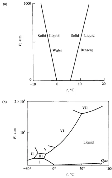
High-pressure chemistry leads to more than just simple extensions of diagrams such as Fig. 8-8(a). Reactions become feasible that do not occur ordinarily, such as the conversion of graphite into diamonds (small ones) and the formation of new types of crystal phases. The water system now looks as shown in Fig. 8-8(b). At around 2000 atm, the ordinary hexagonal structure of ice rearranges, that is, undergoes a phase transition, to a different and denser crystal structure known as
FIG. 8-8. (a) Variation of melting point with pressure for water and for benzene, (b) Phase map or phase diagram for water, including the various high-pressure forms.
ice III. The freezing point curve now slopes to the right. Further phase transitions take place at successively higher pressures to give ice V, ice VI and, finally, ice VII.
Equation (8-6) applies also to transitions between two solid phases and governs the lines showing the effect of pressure on the transition temperature between any two of the solid forms of ice. The figure has taken on the appearance of a phase map.
At a temperature below a two-phase equilibrium line only the lower-temperature phase is present; conversely, at a temperature to the right of the line only the higher-temperature phase exists. The various marked regions thus each consist of a single phase only and the boundaries are lines of two-phase equilibrium.
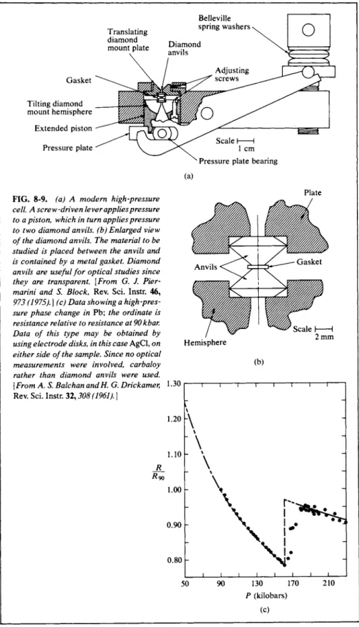
An interesting current story is that of the development of the phase diagram for C(graphite), C(liquid), and diamond. The key to the synthesis of diamond from graphite, incidentally, has been the inclusion of catalysts, along with the use of high temperature and pressure. Figure 8-9 shows an example of a modern piece of high-pressure equipment. Such devices can be compact. A diamond anvil unit capable of producing 105 atm pressure can, for example, be held in the hand.
We return to the low-pressure region to include the liquid-vapor equilibrium
Translating diamond mount plate
Belleville spring washers >
Gasket Tilting diamond mount hemisphere
Extended piston Pressure plate
FIG. 8-9. (a) A modern high-pressure cell. A screw-driven lever applies pressure to a piston, which in turn applies pressure to two diamond anvils, (b) Enlarged view of the diamond anvils. The material to be studied is placed between the anvils and is contained by a metal gasket. Diamond anvils are useful for optical studies since they are transparent. [From G. J. Pier- marini and S. Block, Rev. Sci. Instr. 46, 973 (1975). ] (c) Data showing a high-pres
sure phase change in Pb; the ordinate is resistance relative to resistance at 90kbar.
Data of this type may be obtained by using electrode disks, in this case AgCl, on either side of the sample. Since no optical measurements were involved, carbaloy rather than diamond anvils were used.
[From A. S. Balchan andH. G. Drickamer, Rev. Sci. Instr. 32,308 (1961). \
1 cm
s Pressure plate bearing (a)
Plate
Hemisphere 2 mm
(b) 1.30
1.20
1.10 h R
^ 9 0 1.00 h
0.90
0.80 h
50 90 130 170 210 Ρ (kilobars)
(c)
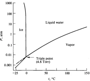
line in the phase map for water, shown schematically in Fig. 8-10. Included as well is the ice-vapor equilibrium line, or the plot of the sublimation pressure of ice versus temperature to which the Clausius-Clapeyron equation (8-8) applies. The pressure scale of a diagram of this sort has a dual significance. In the case of the solid-vapor and liquid-vapor lines, pressure is the vapor pressure of the phase in question. For the solid-liquid line, however, no vapor phase is present, and pressure is now mechanically applied pressure.
Note that the solid-vapor line is steeper than the liquid-vapor line; this is because the enthalpy of sublimation is greater than that of vaporization of the
F I G . 8 - 1 1 . Phase diagram for sulfur. Dashed lines represent metastable equilibria.
95 125
/, ° C
FIG. 8-10. Phase diagram for water in the low-pressure region, showing the ice I-liquid-vapor triple point at 4.6 Torr.
liquid. This must always be so:
(a) solid = liquid, (b) liquid = vapor,
f 5
(8-16) (c) = (a) + (b) solid = vapor, ΔΗ% = AHt + ΔΗν .
Δ Ha must be the sum of Δ Hi and ΔΗν , and since both are positive, the conclusion follows that ΔΗβ > ΔΗν. One consequence is that the solid-vapor and liquid- vapor lines must cross in the manner shown. In the case of water, they do so at 0.0099°C and at the common vapor pressure of 4.579 Torr. This crossing is known as the triple point since three phases are in equilibrium: solid, liquid, and vapor.
A further consequence is that the solid-liquid equilibrium line must also cross the other two at the triple point. The general rule is that any triple point marks the intersection of the lines representing the three ways of taking two phases at a time.
Figure 8-8(b), for example, shows several triple points.
The subject of phase equilibria and phase maps, commonly called phase diagrams, is taken up in Chapter 11. However, one other often encountered phase diagram is that for sulfur, shown in Fig. 8-11. The pressure scale is somewhat schematic, so as to make the diagram more easily displayed. Below 95°C rhombic sulfur is the stable crystal modification and line ab gives the sublimation pressure for this form.
Transformation to monoclinic sulfur occurs at 95°C and line be gives its sublimation pressure: point b is then the rhombic-monoclinic-vapor triple point. Monoclinic sulfur melts at about 125°C and the vapor pressure of liquid sulfur is given by segment cd. A second triple point, at c, marks the monoclinic-liquid-vapor point.
Rhombic sulfur is denser than monoclinic sulfur so the two-phase equilibrium line be slopes to the right; and monoclinic sulfur is denser than the liquid, so that line ce also slopes to the right. The relative slopes are such, however, that the two lines intersect at point e, a third triple point, at which one has a rhombic-monoclinic- liquid equilibrium.
An additional aspect shown in Figs. 8-10 and 8-11 is metastable phase equilibrium.
Thus liquid water may be cooled below its freezing point (to as low as — 40°C);
the liquid-vapor line in this region represents a metastable equilibrium since the liquid is unstable toward freezing. Such lines are shown in the figures as dashed lines. In the water diagram the extension of the liquid-vapor line is possible;
a solid cannot be metastable toward melting, however, nor can a liquid or a solid be metastable toward establishing an equilibrium vapor pressure. However, one crystal modification can be metastable with respect to another. Thus rhombic sulfur can be heated above 95°C without immediately converting to the more stable monoclinic form; its metastable vapor pressure curve is given by line bf in Fig. 8-11. Liquid sulfur can be supercooled along line cf. The diagram therefore shows a fourth, metastable triple point for the rhombic-liquid-vapor equilibrium.
This completes the possibilities; that is, four phases can show a maximum of six two-phase equilibrium lines and four triple points. A triple point may be entirely hypothetical, however, and not just metastable. For example, if rhombic sulfur happened to be less dense than monoclinic sulfur, line be of Fig. 8-11 would then slope to the left, and the rhombic-monoclinic-liquid triple point would be a hypothetical or totally unstable one lying somewhere in the vapor phase region.
F I G . 8-12. Plot ofG as a function of Ρ and Τ for a liquid and its vapor. The crossing of the two surfaces marks the line of liquid-vapor equilibrium and hence gives vapor pressure versus tem
perature for the liquid.
8-5 The Free Energy of a Liquid and Its Vapor
Equation (8-1) gives Gg as a function of Γ and P; values of (Gg — E0) (E0 being the internal energy at 0 K) can be obtained, for example, from the spectro
scopic constants for the gas, using the appropriate partition functions, as discussed in the preceding chapter. The graphical display of Gg would look approximately as shown in Fig. 8-12; Ge decreases with increasing temperature and increases with increasing pressure. The function Gt for the liquid is not easily evaluated theoret
ically but should have the qualitative appearance shown in the figure; the pressure dependence should be much less than for Gg , for example, and at low temperatures the surface must lie below that for Gg since the liquid is then the stable phase. We also know that the line of intersection of the two surfaces must correspond to the P-T line of liquid-vapor equilibrium. A third surface for G8 also exists; its inter
section with the other two would give the solid-liquid and solid-vapor equilibrium lines.
Along the liquid-vapor line, then, Gg = Gt, and a convenient way of describing Gi is in terms of the free energy of the vapor. We ordinarily deal with vapor pressures not much over 1 atm and will therefore make the assumption that the vapor behaves ideally. The free energy of a gas is given by Eq. (6-49), which becomes, in the present context,
dGg = RT d{ln P) (ideal gas) (8-17)
or
Gg = Gg° + RTln Ρ (ideal gas) (8-18)
for a change in pressure at constant temperature. Here Gg° is the free energy of
8-6 The Surface Tension of Liquids.
Surface Tension as a Thermodynamic Quantity
We have so far considered only bulk properties, that is, properties of a portion of matter which, if extensive, are proportional to the amount of substance or which, if intensive, apply to the interior of the phase. We now recognize that energy resides in the interface between two phases and, more specifically, that work is required to form or to extend an interface. For the present, the discussion is limited to the liquid-vapor interface of pure liquids. The treatment of solutions is deferred to Section 9-ST-2.
The requirement of work to increase a liquid-vapor surface is most easily demonstrated experimentally by means of soap films, since these persist long enough to be handled. As illustrated in Fig. 8-13(a), if a soap film is formed in a the vapor or gas phase at the temperature in question and 1 atm pressure, and is thus the standard-state free energy. It follows that
Gt° = Gg° + RTlnP°, (8-19)
where Gi° is the free energy of the liquid in its standard state and P° is the liquid vapor pressure. Strictly speaking, Gt° refers to the liquid under its own vapor pressure, but the small difference between this value and that for the usual standard state of 1 atm pressure can be neglected here.
Equation (8-19) will be very useful in dealing with solutions. An immediate application is as follows. Returning to Eq. (8-2), we see that the free energy of a liquid increases with pressure at constant temperature; integration gives
Git2 = G° + Γ Vl dP~GQ + Vl ΔΡ, (8-20)
J po
where P° is the vapor pressure of the liquid and Ρ is some imposed mechanical pressure. If this higher pressure is established by using an inert gas to compress the liquid, there will still be a gas phase and the liquid will still have an equilibrium vapor pressure P°'. This vapor pressure P°' corresponds to a vapor free energy of Gg° + RT In P°', so we have
Gl2 = Gg° + RT In (8-21)
On combining Eqs. (8-19)—(8-21), we obtain
RT In 4ΪΓ = Γ Vi dP ~ Vx ΔΡ. (8-22)
Γ J po
Returning to Fig. 8-12, Glt2 corresponds to point a located on the free energy surface for the liquid at temperature Τ and mechanical pressure P2. The vapor having the same free energy at Τ is in the state given by point b, or at vapor or gas pressure P°'.
A numerical illustration is as follows. Water has a molar volume of 18 c m8 m o l e- 1 and if w e neglect its compressibility, then for 100 atm pressure, the integral of Eq. (8-22) is just (18)(100) = 1800 c m8 atm. A t 2 5 ° C , RT = (82.06)(298.2) = 24,470 c m8 a t m and l n ( P0 ,/ P0) b e c o m e s (1800)/
(24,470) = 0.0736 and P°'/P° = 1.076. T h e vapor pressure is thus increased 7.6% by the application o f 100 a t m pressure.
F I G . 8-13. Work of extending a surface: (a) Extending a soap film held in a wire frame by moving a side, (b) Extending the surface of a liquid by sliding back a cover of inert material.
frame one side of which can move freely, one finds that the film will spontaneously contract, and that to prevent contraction, a f o r c e / m u s t be applied. If / i s decreased slightly, contraction occurs, and if / is increased, the film extends. The process is then a reversible one, and the work involved is reversible, constant-temperature and constant-pressure work. It therefore corresponds to a free energy quantity.
For a small displacement dx of the movable side of the frame the work done by the film is
where γ is the force per unit length exerted by the film and is called the surface tension. The units of surface tension are evidently force per unit length, or, in the cgs system, dyne per centimeter. Since / dx is the change in area of the film ds/, a less geometrically specific form of Eq. (8-23) is
Evidently, γ can also be expressed in units of energy per unit area, or as erg per square centimeter. The two sets of units are equivalent, and surface tension may be stated in either way. The experiment with a pure liquid, rather than a soap solution, is the hypothetical one shown in Fig. 8-13(b). We imagine a container filled with the liquid and at a given Τ and P. There is a movable lid that can be slid back and forth to change the amount of liquid surface. (We stipulate that there is no inter
action between the liquid and the material of the lid.) The force on the lid is then yl as before.
The free energy change associated with a change in surface area can be added to the usual statement of the combined first and second laws [Eq. (6-43)] to give
w = —f dx = —yl dx, (8-23)
= —yds/. (8-24)
dG = -SdT+ VdP + γ dsf. (8-25)
Thus
y = ( w )r. , = °s> <8-2 6>
where GB denotes the surface free energy per unit area. Further, since the process of Fig. 8-13(b) is a reversible one, the q associated with it is a qrey , and we have
dq = TdS= TS* d&, (8-27) where SB is the surface entropy, also per unit area. Other thermodynamic relation
ships apply. By Eq. (6-45), (dG/dT)P = - 5 , and likewise,
3G8
'p or
Also
HB = GB + TSB. (8-29)
Often, and as a good approximation, HB and the surface energy EB are not distin
guished, so Eq. (8-29) is usually given in the form
E*=G* + TSB (8-30)
or
EB = γ - T ^ (8-31)
(constancy of pressure being assumed for dy/dT).
The thermodynamics of curved interfaces constitutes a very important topic, one aspect of which is developed here. This is known as the Laplace equation and relates the mechanical pressure across an interface and its curvature. To illustrate the physical reality of the effect, we again use a soap film, now in the form of a soap bubble. As shown in Fig. 8-14, a manometer is attached to the soap bubble pipe, and after the bubble has been blown, the stem of the pipe is closed off. The manometer will now show a pressure difference. For an actual soap bubble this is about 1mm H2O f o r a bubble of 2 mm radius. The physical explanation for the higher pressure inside the bubble is that the film tends spontaneously to decrease its area and hence its total surface free energy but, in doing so, shrinks the bubble to the point that the increased pressure prevents further change.
The relevant equation may be derived as follows. Consider a bubble of radius R as shown in Fig. 8-14(b). Its total surface free energy is AnR2y and if the radius were to decrease by dR, then the change in surface free energy would be SnRy dR. Since shrinking decreases the total surface free energy, at equilibrium the tendency to shrink must be balanced by a pressure difference across the film Δ Ρ such that the work against this pressure difference (AP)4nR2 dR is just equal to the decrease in surface free energy. Thus we have
( J P) 4T T ^2 dR = SwRy dR
(b)
F I G . 8-14. (a) The pressure inside a soap bubble is larger than that outside, (b) Derivation of the Laplace equation for a spherical surface.
or
ΔΡ = Ο-. (8-32)
Equation (8-32) is the Laplace equation for a spherical interface. An important conclusion is that the smaller the bubble, that is, the smaller the value of R9 the larger is ΔΡ. Conversely, J P goes to zero in the limit of R - > o o , which corresponds to the case of a plane interface.
Parenthetically, c o m m o n usage defines γ as the surface tension for o n e interface. Because of this it would be better to use 2y instead of y in relationships such as Eq. (8-32) when they are applied to soap or other films.
In summary, the two most important relationships developed so far are Eq. (8-31) for surface energy, EB = γ — T(dy/dT)9 and the Laplace equation (8-32), ΔΡ = Ιγ/R. The latter is one of the four principal special equations of surface chemistry, the other three being the Kelvin equation (Section 8-9), the Gibbs equation (Section 9-ST-2), and Young's equation [see Adamson (1976)].
8-7 Measurement of Surface Tension
We do not usually devote much space to experimental procedures, but the various ways of measuring surface tension are so closely related to basic surface phenomena that discussion of the former illustrates the latter.
F I G . 8-15. (a) The capillary rise phe
nomenon, (b) Detail for the case of a spherical meniscus.
A. Capillary Rise
If a small-bore tube is partially immersed in a liquid as shown in Fig. 8-15(a), one usually observes that the liquid rises to some height h above the level of the general liquid surface. This phenomenon may be treated by means of the Laplace equation. If, as shown in more detail in Fig. 8-15(b), the liquid wets the wall of the capillary tube, then if the radius of the tube r is small, the meniscus will be hemi
spherical in shape. Its radius of curvature is then equal to r, that is, R = r, and Eq. (8-32) becomes
ΔΡ = . (8-33)
If, as further illustrated in the figure, Px is the general atmospheric pressure, then the pressure just under the meniscus must be P j — (2y/r). The J P in the Laplace equation is always such that the higher pressure is on the concave side of the curved surface. The pressure Px is also the pressure on the flat portion of the liquid surface outside the capillary tube, and hence the pressure at that liquid level inside the capillary. Then P1 — P2 must correspond to the change in hydrostatic pressure of
the liquid, pgh. We can thus write
Pgh = ^~ (8-34)
or
(8-35) (Strictly speaking, one should use Δρ9 the difference in density between the liquid and vapor phases.) The quantity Ιγ/pg is a property of the liquid alone and Eq.
(8-35) may be put in the form
where a is called the capillary constant. Equation (8-36) tells us that the plot of capillary rise h versus r is a hyperbola. Equation (8-36) is exact only in the limit of small r; otherwise corrections are needed.
A more general case is that in which the liquid meets the capillary wall at some angle θ as illustrated in Fig. 8-16. Without going through the details of the geom
etry, we can say that the radius of curvature of the meniscus R is now given by R = r/cos θ (assuming the meniscus is still spherical in shape) and Eq. (8-35) becomes
A liquid making an angle of 90° with the wall would show no capillary rise at all.
Mercury, whose contact angle against glass is about 140°, shows a capillary depression. That is, cos θ is now negative and so is h.
The following is an alternative approach, but one which is equivalent to the preceding in the first approximation. The spontaneous contractile tendency of a liquid surface acts as though there were a surface force γ per unit length. In the capillary rise situation, the total such force is 2nry (or, more generally, the vertical component would be lirry cos Θ). This force is balanced by the force exerted by gravity on the column of liquid which is supported, or {frrr2){pgh). On equating these
two forces, we have Eq. (8-34) [or (8-37)].
a2 = rh9 (8-36)
h = 2γ cos θ
pgr (8-37)
F I G . 8-16. Capillary rise in the case of a nonwetting liquid. Detail shows the meniscus profile assuming a spherical shape.
F I G . 8-17. Mechanism of water repellancy.
The capillary rise phenoJmenon is not only the basis for an absolute and accurate means of measuring surface tension but is also one of its major manifestations.
The phenomenon accounts for the general tendency of wetting liquids to enter pores and fine cracks. The absorption of vapors by porous solids to fill their capillary channels and the displacement of oil by gas or water in petroleum formations constitute specific examples of capillarity effects. The waterproofing of fabrics involves a direct application of Eq. (8-37). Fabrics are porous materials, the spaces between fibers amounting to small capillary tubes. As shown in Fig.
8-17(a), coating the fibers with material on which water has a contact angle of greater than 90° provides a Laplace pressure which opposes the entry or "rise" of water into the fabric. The material is not waterproof; once the Laplace pressure is exceeded (as, for example, by directing a jet of water onto the fabric o r merely by rubbing of the wet fabric), then penetration occurs, and water will seep freely through the filled channels as illustrated in Fig. 8-17(b).
β. D r o p Weight M e t h o d
It was pointed out earlier that one can assign a force γ per unit length of a liquid surface as giving the maximum pull the surface can support. In the case of a drop of liquid which is formed at the tip of a tube and allowed to grow by delivering liquid slowly through the tube, a size is reached such that surface tension can no longer support the weight of the drop, and it falls. The approximate sequence of
F I G . 8-18. Sequence of shapes for a drop that detaches from a tip. [From A. W. Adamson,
"The Physical Chemistry of Surfaces" 3rd ed. Copyright 1976, Wiley {Interscience), New York.
Used with permission of John Wiley & Sons, Inc.]
shapes is shown in Fig. 8-18. To a first approximation, we write
^ideal = 2nry, (8-38) where FKideai denotes the weight of the drop that should fall and r is the radius of
the tube (outside radius if the liquid wets the tube). Equation (8-38) is known as Tate's law.
As also illustrated in the figure, the detached drop leaves behind a considerable residue of liquid, and the actual weight of a drop is given by
^act = ^ideal/, (8-39) where / is a correction factor which can be expressed either as a function of r/a,
where a is the square root of the capillary constant, or of r/K1/3, where V is the volume of the drop. Table 8-2 gives some values of / ; a more complete table is given in the reference cited therein. Note that the correction is considerable. The method, using the correction table, is accurate and convenient, however. In practice, one forms the drops within a closed space to avoid evaporation and in sufficient number that the weight per drop can be determined accurately. It is only necessary to form each drop slowly during the final stages of its growth.
C. Detachment Methods
A set of methods that are somewhat related in treatment to the drop weight method have in common that one determines the maximum pull to detach an
T A B L E 8-2. Correction Factors for the Drop Weight Methoda
/ r/yi/z f
0.30 0.7256 0.80 0.6000
0.40 0.6828 0.90 0.5998
0.50 0.6515 1.00 0.6098
0.60 0.6250 1.10 0.6280
0.70 0.6093 1.20 0.6535
a See A . W . A d a m s o n , "Physical Chemistry o f Sur- faces," 3rd ed. Wiley (Interscience), N e w Y o r k , 1976.
F I G . 8-19. The Wilhelmy slide method. A thin plate is suspended from a balance.
object from the surface. If the perimeter of the object is p, then the maximum weight of meniscus that the surface tension can support is just
^ i d e a l = ργ. (8-40)
The so-called du Nouy tensiometer uses a wire ring, usually made of platinum, and ρ is then 4nR9 where R is the radius of the ring, and one is allowing for both the inside and the outside meniscus. As with the drop weight method, rather large correction factors are involved, and these have been tabulated [see Adamson (1976)].
If, instead of a ring, one uses a thin slide, either an actual microscope slide or a metal one of similar size, then it turns out that Eq. (8-40) is quite accurate and may be applied directly. The method is now known as the Wilhelmy slide method and is shown schematically in Fig. 8-19. Alternatively, the slide need not be detached but need merely be brought into contact with the liquid and then raised until the end is just slightly above the liquid surface. The extra weight is again the meniscus weight and is given by Eq. (8-40). The Wilhelmy method is one of those most widely used today. It is especially valuable in studying the surface tension of solutions and of films of insoluble substances.
8-8 Results of Surface Tension Measurements
Some representative surface tension values are assembled in Table 8-3. Notice the very wide range in values, from 0.308 dyn c m- 1 for liquid helium to 1880 dyn c m- 1 for molten iron. An important datum is the value for water, 72.88 dyn c m "1 at 20°C; other common solvents have surface tensions around 20-30 dyn c m- 1. Some values for the interfacial tension between two liquids are included. The SI unit of surface tension is newton per meter ( N m "1) ; l N m ~1 = 103 dyn c m "1.
O n e m a y use the table t o illustrate characteristic values in the various m e t h o d s for determining surface tension. F o r example, the constant a2 is 0.15 c m2 for water, about 0.05 c m2 for a typical organic liquid, and around 0.5 for a m o l t e n metal. E q u a t i o n (8-36) then allows a n easy estimate o f the capillary rise. T h u s , for water in a 0.1-cm-diameter capillary, h = 0.15/0.05 = 3.0 c m and for a 0.01-cm-diameter capillary, h = 30 c m .
H a d the drop weight m e t h o d been used, a n average weight o f a b o u t 0.085 g w o u l d h a v e been f o u n d using a tip o f 0.3 c m outside radius. T h e quantity rjVllz is 0.68 and from Table 8-2,