Cost Sharing Models in Game Theory

(1)

Cost Sharing Models in Game Theory

PhD Thesis

by

Anna Ráhel Radványi

Doctoral School of Economics, Business and Informatics Corvinus University of Budapest

Supervisors:

István Deák, DSc

Department of Computer Science

Institute of Information Technology, Corvinus University of Budapest

Miklós Pintér, PhD Institute of Mathematics

Budapest University of Technology and Economics;

Department of Operations Research and Actuarial Sciences

Institute of Mathematics and Statistical Modelling, Corvinus University of Budapest

Corvinus University of Budapest 2020

(2)

List of Figures

2.1 Ditch represented by a tree-structure in Example 2.4 . . . 7

2.4 Tree structure in Example 2.28 . . . 20

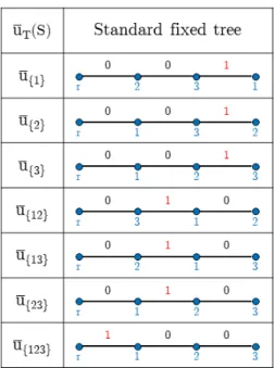
4.1 u¯_T(S) games represented as standard xed trees . . . 41

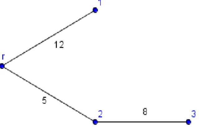
4.2 Fixed tree network in Example 4.7 . . . 42

5.1 Cost tree (G, c) of irrigation problem in Example 5.2 . . . 53

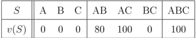
5.2 Cost tree (G, c) of airport problem in Example 5.5 . . . 54

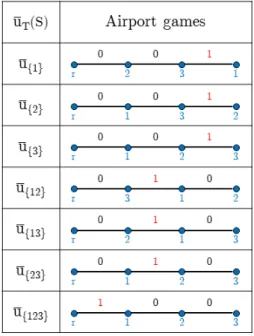
5.3 Duals of unanimity games as airport games . . . 55

5.4 Cost tree (G, c) of irrigation problems in Examples 5.2 and 5.9 . . 56

6.1 Cost tree (G, c) of UR game in Example 6.2 . . . 73

6.2 Duals of unanimity games as UR games . . . 73

6.3 Duals of unanimity games as irrigation and UR games . . . 75

7.1 Graph of shortest path cooperative situation in Example 7.7 . . . 86

(5)

List of Tables

2.1 Properties of allocations . . . 14

3.1 The horse market game . . . 32

3.2 The horse market game and its Shapley value . . . 35

7.1 Shortest path game induced by Example 7.7 . . . 87

(6)

Notations

Cost allocation models

N ={1,2, . . . , n} the nite set of players L ⊆N the set of leaves of a tree

i ∈N a given user/player

c_i the cost of the ith segment/edge

I_i⁻ ={j ∈N|j < i}the set of users preceding i I_i⁺ ={j ∈N|i < j}the set of users following i ξ_i^a the average cost allocation rule

ξ_i^s the serial cost allocation rule

ξ_i^eq the allocation rule based on the equal allocation of the non-separable cost ξ_i^riu the allocation rule based on the ratio of individual use of the non-

separable cost

ξ_i^r the restricted average cost allocation rule Introduction to cooperative game theory

TU game cooperative game with transferable utility

|N| the cardinality of N

2^N the class of all subsets ofN A⊂B A⊆B, but A6=B

A]B the disjoint union of sets A and B

(N, v) the cooperative game dened by the set of players N and the characteristic function v

v(S) the value of coalition S ⊆N

G^N the class of games dened on the set of players N

the cost game with the set of players and cost function

(7)

I^∗(N, v) the set of preimputations I(N, v) the set of imputations

C(N, v);C(v) the set of core allocations; the core of a cooperative game X^∗(N, v) =

x∈R^N| x(N)≤v(N) , the set of feasible payo vectors ψ(v) = (ψi(v))i∈N ∈R^N, the single-valued solution of a game v v⁰_i(S) =v(S∪ {i})−v(S), the player i's individual marginal contri-

bution to coalition S

φ_i(v) the Shapley value of player i

φ(v) = (φi(v))i∈N the Shapley value of a game v π an ordering of the players

ΠN the set of the possible orderings of set of playersN Fixed tree games

Γ(V, E, b, c, N) a xed tree network

G(V, E) directed graph with the sets of nodes V and edges E

r ∈V the root node

c the non-negative cost function dened on the set of edges Si(G) = {j ∈V :i≤j} the set of nodes accessible from i via a di-

rected graph

Pi(G) = {j ∈ V : j ≤ i} the set of nodes on the unique path connecting i to the root

S¯ the trunk of the tree containing the members of coalition S (the union of unique paths connecting nodes of members of coalition S to the root)

u_T the unanimity game on coalition T

¯

uT the dual of the unanimity game on coalition T Airport and irrigation games

(G, c) the cost tree dened by the graph Gand cost function c G_I^A the class of airport games on the set of players N

G_I^N the class of irrigation games on the set of players N

(8)

GG the subclass of irrigation games induced by cost tree problems dened on rooted tree G

Cone {vi}i∈N the convex cone spanned by given vi games i− ={j ∈V :ji∈E} the player preceding player i virr the irrigation game

i∼^v j i and j are equivalent players in game v, i.e. v_i⁰(S) =v⁰_j(S) for all S⊆N \ {i, j}

ξ^SEC sequential equal contributions cost allocation rule Upstream responsibility

ij~ the directed edge pointing from i toj

E_i the set of edges whose corresponding emissions are the direct or indirect responsibility of i

ES the set of edges whose corresponding emissions are the direct or indirect responsibilities of players inS

G_{U R}^N the class of UR games corresponding to the set of players of N Shortest path tree games

Σ(V, A, L, S, T) the shortest path tree problem

(V, A) directed, acyclic graph dened by the sets of nodes V and edges A

L(a) the length of the edge a

S ⊆N the nonempty set of sources T ⊆N the nonempty set of sinks

P the path connecting the nodes of{x₀, . . . , x_p} L(P) the length of path P

o({x}) function dening the owners of node x

o(P) denes the owners of the nodes on the path P

g the income from transporting a good from a source to a sink σ(Σ, N, o, g) the shortest path cooperative situation

v_σ the shortest path game

(9)

Acknowledgements

There is a long journey leading to nishing a doctoral thesis, and if we are lucky, we are not alone on this journey. Our companions are our families, friends, men- tors, all playing an important role in shaping how dicult we feel the journey is.

When arriving at a crossroads they also undoubtedly inuence where we go next.

My journey started in primary school, when mathematics became my favorite subject. My silent adoration for the principle was rst truly recognized by Milán Lukovits (OFM), it was him who started my career as a mathematician, and also saw my passion for teaching. I am thankful to him for his realization and provocative remarks that made me eventually build up my courage to continue my studies as a mathematician. The other highly important gure of my high school years was László Ern® Pintér (OFM) who not only as a teacher, but a recognized natural sciences researcher has passed on values to his students such as intellectual humility, modesty, and commitment to research of a high standard.

These values stay with me forever, no matter where I am.

I am very grateful to my supervisors, István Deák and Miklós Pintér. I have learned a lot from István Deák, not only within the realm of doctoral studies, but beyond, about the practical aspects of research, what a researcher at the beginning of her career should focus on. I would like to thank him for his wisdom, professional and fatherly advice, I am grateful that his caring attention has been with me all along. I am deeply grateful to Miklós Pintér, whose contributions I probably could not even list exhaustively. At the beginning he appointed me as teaching assistant, thereby in practice deciding my professional career onward. In the inspiring atmosphere he created it has been a great experience working with him rst as a teaching assistant, and later as a researcher, together with his other students. He has started the researcher career of many of us. He has troubled

(10)

himself throughout the years helping me with my work. I can never be grateful enough for his professional and friendly advice. I thank him for proof-reading and correcting my thesis down to the most minute details.

I am thankful to Béla Vízvári for raising what has become the topic of my MSc, and later PhD thesis. I would like to thank Gergely Kovács for supervising my MSc thesis in Mathematics, and later co-authoring my rst publication. His encouragement has been a great motivation for my starting the doctoral program.

Our collaboration is the basis of Chapter 2.

I am thankful to Judit Márkus for our collaboration whose result is Chapter 5.

I am very grateful to Tamás Solymosi, who introduced me to the basics of cooperative game theory, and László Á. Kóczy. I thank both of them for giving me the opportunity to be a member of their research groups, and for their thoughtful work as reviewers of my draft thesis. Their advice and suggestions helped a lot in formulating the nal version of the thesis.

I will never forget the words of György Elekes from my university years, who at the end of an exam thanked me for thinking. He probably never thought, how many low points his words would help me get over. I am thankful for his kindness, a rare treasure. I would like to thank my classmates and friends Erika Bérczi- Kovács, Viktor Harangi, Gyuri Hermann, and Feri Illés for all the encouragement, for studying, and preparing for exams together. Without them I would probably still not be a mathematician. I thank Eszter Szilvási not only for her friendship, but also for preparing me for the economics entrance exam.

I could not imagine my years spent at Corvinus University without Balázs Nagy. His friendship, and our cheerful study sessions have been with me up to graduation, and later to nishing the doctoral school. We have gone through all important professional landmarks together, he is an exceptional friend, and great study partner. I thank him for having been mathematicians among economists together.

I thank my classmates Peti Vakhal, Tomi Tibori, Laci Mohácsi, and Eszter Monda for making the years of my doctoral studies colorful.

I am indebted to my colleagues at the Department of Mathematics for their support. I would like to thank especially Péter Tallos, Attila Tasnádi, Kolos Ágos-

(11)

ton, Imre Szabó, and Dezs® Bednay. Without their support this dissertation could not have been nished on time.

I am grateful to my family, especially the family members in Szentendre for their support and encouragement. I would like to thank my husband, Ádám Sipos, for always helping me focus on the important things. I thank him for his support and his help in the nalization of the thesis. I thank our children, Balázs and Eszti for their patience, understanding, and unconditional love.

I dedicate this thesis to the memories of my parents and grandparents.

(12)

Foreword

Dear Reader,

When someone asks me what I do, usually my short answer is: I'm researching cooperative game theory. Having given this answer, from members of the general public I usually get more questions, so I tend to add that I attempt to distribute costs fairly. This is usually an attention grabber, because it seems to be an understandable, tangible goal. From this point we continue the discussion and the questions I get (in case the person is still interested, of course) are usually the following. What kind of costs are these? Among whom are we distributing them? What does fair mean? Is there a fair allocation at all? If yes, is it unique?

Can it be easily calculated?

The rst two questions are interrelated: in a specic economic situation costs arise, if there are participants that perform some activity. This is usually easy to word when we have a concrete example. Those without deeper mathematical knowledge usually stop at these two questions. However, modeling itself is already an important mathematical step. Since we are discussing concrete and (many times) common situations, we do not necessarily think that describing the situation, the participants, and their relationships has in eect given the (prac- tically mathematical) answer to two simple, everyday questions. In other words, modeling does not necessarily require complex mathematical methods. As an example, let us consider an everyday situation, building a water supply network in a village. This network connects to a provider source, and the entire water supply network branches o from this point. It is easy to imagine what this system might look like: from a linear branch further segments branch o providing access to water for all residents. Of course, there are no circles in this system, it is suf-

(13)

tree structure. However, this system must be built, maintained, and so forth. We can already see the costs that the residents of the village will have to pay for, therefore we have now dened the agents of the model as well. The structure of the network describes the relationships among the agents, which is essential for the distribution.

Let us consider the next question, fairness. Not everybody might phrase the question as what makes a distribution fair. Clearly, the costs must be covered by someone(s). Let us give a distribution for this implicit requirement. Those more interested in the topic may also be curious about the mathematician's expected complicated answer to a question that seems so simple. Instead, the mathematician replies with a question: What should the distribution be like?

More precisely, what conditions should it satisfy? What do we expect from the distribution? That the entire cost is covered? Is this sucient? Would it be a good answer that the last house in the village should pay for all the costs? In the end, it is because of this resident that such a long pipeline must be built. What if the resident is (rightfully) displeased with this decision, is not willing to pay, and instead chooses not to join the system? This may delay, or even halt the entire project, for which external monetary funding could be acquired only if everybody joins and the entire village is covered by the network. How about considering another alternative then, let us make everybody pay evenly. This could be an ac- ceptable solution, but after giving it more consideration we might nd that this solution is also unfair to a certain degree. It is possible that the rst resident in the system now pays more than as if it was building the system alone, therefore in practice the resident subsidizes those further back in the system. There is no clear advantage to be gained from such a setup, what's more, it may be downright undesirable for the resident. Therefore, it is yet another rightful expectation that all participants' payments should be proportional to the segments they use in the water supply network. Those closer to the source should pay less, and those further back should pay more, since they use a larger section of the system. Several further aspects could be taken into consideration (e.g. the quantity of water used by the participants, these are the so called weighted solutions). It is the modeler's task to explore the requirements and customize the solution to the specic prob-

(14)

lem, adding conditions regarding the distribution to the model. These conditions will be given in the form of axioms, and for each solution proposal it must be examined whether it satises the axioms and therefore the expectations as well.

The next step is the question of existence. Is it at all possible to give a solution that satises all expected properties, or has the denition been perhaps too strict, too demanding? Namely, in certain cases some conditions cannot all be satised at the same time. Then we need to do with less, and after removing one (or more) conditions we can look for solutions that satisfy the remaining conditions.

Of course, this raises the question, which condition(s) we want to remove, which are removable, if at all. This is not a simple question and always depends on the specic model, the modeler, and the expectations as well. In some fortunate cases, not only one, but multiple solutions satisfy the expected properties. Then we can analyze what further good properties these solutions possess, and choose the ttest for our purposes accordingly. Probably the most favorable cases are those for which there is exactly one solution, in other words, the distribution solving the problem is unique. Therefore, there are no further questions, choices, or any aspects to be debated. The answer is given, unambiguous, and therefore (probably) undisputable.

The last question to be raised is just as important, if not more so, than the previous ones. We have created the model, dened the problem, the requirements, and have even found a theoretical solution. But can it be calculated? Can the solution be implemented in practice? What is the use of a solution, if we can never learn, how much the participants really have to pay? It can happen that there are too many participants, the model is too complex, the network is too large, and we cannot arrive at a precise number for the solution even by leveraging computers and algorithmic methods. Fortunately, in several cases the structure of the network is such that in spite of its vastness, an ecient algorithm exists for computing a concrete solution. These problems belong to the area of computational complexity.

In the present thesis we will examine these questions for specic types of situations, focusing primarily on the denition of fairness. We analyze the theory behind models of several economic problems, and give answers applicable

(15)

in practice to the questions raised regarding distribution. As we progress from question to question in the case of specic situations, the methodology will seemingly become increasingly more abstract, the answers more theoretical. All along, however, we do not lose sight of our main objective: providing fair results applicable in practice as a solution. What does cooperative game theory add to all this? It adds methodology, models, axioms, solution proposals, and many more.

The details emerge in the following chapters. Thank you for joining me!

(16)

Chapter 1 Introduction

In the present thesis we examine economic situations that can be modeled using special directed networks. A special network in Chapters 2, 4, 5, and 6 will trans- late into rooted trees, while in Chapter 7 will mean directed, acyclic graph. Even though the basic scenarios are dierent, we will be looking for answers to similar questions in both cases. The dierence stems only from the relationships of the agents in the economic situation. Namely, we will be examining problems where economic agents (companies, individuals, cities, states, so forth) collaboratively create (in a wider sense) an end product, a measurable result. Our goal is to fairly distribute this result among the players.

For example, we will be discussing situations, where a group of users are provided a service by a utility (e.g. water supply through an infrastructure). A network (graph) comprises all users, who receive the service through this network. The building, maintenance, and consuming of the service may incur costs.

Another example is a problem related to the manufacturing and transportation of a product. A graph describes the relationships among suppliers, companies, and consumers during the manufacturing process. In this case, transportation costs are incurred, or prots and gains are achieved from the sales of the product.

In the case of both examples we will be looking for the answer to the question of fairly allocating the arising costs or achieved gains among the participants.

This raises further questions, one is what it means for an allocation to be fair, what properties are expected from a fair allocation? A further important question is whether such allocation exists at all, and if it exists, is it unique? If multiple

(17)

distributions satisfy the criteria, then how should we choose from them? Another important aspect is that we must provide an allocation that can be calculated in the given situation. In the thesis we are going to discuss these questions in the case of concrete models, leveraging the toolset of cooperative game theory.

The structure of the thesis is as follows. After the introduction, in Chapter 2 we are analyzing a real-life problem and its possible solutions. Aadland and Kolpin (2004) studied cost allocation models applied by farmers for decades in the state of Montana, this work is the origin for the average cost-sharing rule, the serial cost sharing rule, and the restricted average cost-sharing rule. We present two further water management problems that arose during the planning of the economic development of Tennessee Valley. We discuss the two problems and their solution proposals (Stran and Heaney, 1981). We formulate axioms that are meant to describe the fairness of an allocation, and we discuss which axioms are satised by the aforementioned allocations.

In Chapter 3 we introduce the fundamental notions and concepts of cooperative game theory, focusing primarily on those areas that are relevant to the present thesis. We discuss in detail the core (Shapley, 1955; Gillies, 1959) and the Shapley value (Shapley, 1953), that play an important role in nding a fair allocation.

In Chapter 4 we present the class of xed-tree games. We provide the rep- resentation of a xed-tree game, and examine what properties the core and the Shapley value of the games possess. We present several application domains stem- ming from water management problems.

In Chapter 5 we discuss the classes of airport and irrigation games, and the characterizations of these classes. Furthermore, we extend the results of Dubey (1982) and Moulin and Shenker (1992) on axiomatization of the Shapley value on the class of airport games to the class of irrigation games. We compare the axioms used in cost allocation literature with the axioms of TU games, thereby providing two new versions of the results of Shapley (1953) and Young (1985b).

In Chapter 6 we introduce the upstream responsibility games and characterize the game class. We show that Shapley's and Young's characterizations are valid on this class as well.

(18)

In Chapter 7 we discuss shortest path games, which are dened on graph structures dierent from those in the previous chapters. After introducing the notion of a shortest path game, we show that this game class is equal to the class of monotone games. Then we present further axiomatizations of the Shapley value, namely Shapley (1953)'s, Young (1985b)'s, Chun (1989)'s, and van den Brink (2001)'s characterizations, and examine if they are valid in the case of shortest path games.

In Chapter 8 we summarize our results.

We will annotate our own results (lemmata, claims, theorems, and new proofs of known theorems) in the thesis by framing their names. The author of present thesis and the co-authors of the publications have participated equally in the work leading to these results.

(19)

Chapter 2 Cost allocation models

This chapter and our entire thesis discusses cost allocation problems. The problem is described as follows. A group of farmers acquire water supply for their land from a ditch that is connected to a main ditch. Operation and maintenance of the ditch incur costs which are jointly covered by the group. The question is how the farmers (henceforth users) may fairly divide the aforementioned costs among the group. After the introduction we shall present the basic models and the axioms aiming to dene the notion of fairness. The axioms are based on the work of Aadland and Kolpin (1998).

The basis of our models are solution proposals for real-life problems. In Aad- land and Kolpin (2004) cost allocation patterns are examined, utilized for decades in practice by Montana ranchers. In their paper they describe two cost allocation mechanisms, the serial and the average cost share rules. Furthermore, they present the restricted cost share method (Aadland and Kolpin, 1998), which uni- es the advantages of the previous two methods. Their results were dened on non-branching trees, i.e. chains.

In this chapter we generalize the above models for problems described by tree- structures, and show that they uphold the properties of cost allocations described for chains. These results were presented in our paper (Kovács and Radványi, 2011, in Hungarian).

The basis of two further models we analyzed are also solution proposals for questions arising in connection with water management problems. The Tennessee Valley Authority was established in 1933 with the purpose of creating the plans

(20)

for the economic development of Tennessee Valley. TVA's work was rst presented in economics and game theory literature by Stran and Heaney (1981), and is the origin for methods based on separable - non-separable costs. The basis for the description of our models is the work of Solymosi (2007) (in Hungarian).

For formal analysis let us rst summarize the two most important properties of the ditch in our example. Firstly, all users utilize water rst and foremost for the irrigation of their own land, and the water quantity required for and costs related to livestock are negligible. Experience shows that the capacity of ditches is sucient for the irrigation of all lands. Therefore, the problem we dene is not the allocation of the water supply, but the allocation of operation, maintenance, and other costs among users.

2.1 Basic models

Let us represent the problem with a tree, let the root of the tree be the main ditch (denoted by r), and let the nodes of the tree be the users. We denote the set of leaves of the tree by L.

LetN ={1,2, . . . , n}be the ordered, nite set of users connected to the main ditch (r /∈N, L⊆ N). There exists a reexive, transitive ordering on the set of users, which is not necessarily a total ordering, since not all two users' positions may be comparable. Let us, for example, consider the access order of a depth-rst search starting from the root of the graph. In this ordering leti denote aith user from the ood gate. Let the ith segment of the ditch (i.e. the ith edge of the graph) be the segment through which theith user connects to the system. For all i ∈N let c_i denote the yearly maintenance cost of the ith segment of the ditch, and let the cost vector dened by these costs be denoted by c = (c_i)_i∈N ∈ R^N+. The sought result is a fair allocation of the summed cost P

i∈Nc_i.

Remark 2.1 In special cases the problem can be represented by a single chain, whose rst node is the main ditch, while the users are the chain's following nodes, and the ordering is self-evident. The associated problem, representable by a single chain, is the well-known airport problem (Littlechild and Thompson, 1977). We discuss this problem, and the associated cooperative game in detail in Chapter 5.

(21)

In the following we dene dierent cost allocation patterns, and examine their inherent properties. For this end we introduce new notations.

For user i we disambiguate between the sets of preceding and following users.

LetI_i⁻ denote the set of nodes residing on the unambiguous path connecting ito the root. This is the set of users preceding i. Let us consider a direction consisting of edges pointing outwards from the root of the tree as source, and exactly one edge directed to each node. In this tree let I_i⁺ denote the set of nodes accessible from ivia a directed path. This is the set of users following i.

In other words, I_i⁻ ={j ∈N|j < i}, I_i⁺={j ∈N|i < j}, where the relation j < i denotes that there exists a directed path from j to i.

In our example we rst examine two cost allocation rules, the (a) average and the (b) serial allocations. Costs may be measured per area in acres, in units of con- sumed water, or per individual user, we will use the latter method. Denition 2.2.

and the axioms presented in this section are based on the work of Aadland and Kolpin (1998).

Denition 2.2 A ξ : R^N+ → R^N+ mapping is a cost allocation rule, if ∀c ∈ R^N+

P

i∈N

ξ_i(c) = P

i∈N

c_i, where(ξ_i(c))_i∈N =ξ(c).

(a) According to the average cost allocation rule the operation and maintenance costs of the ditch are distributed evenly among users, i.e. ∀i∈N:

ξ_i^a(c) =X

j∈N

c_j n

(b) According to the serial cost allocation rule the costs associated with each segment are distributed evenly among those who utilize the segment, i.e. ∀i∈N:

ξ_i^s(c) = X

j∈I_i⁻∪{i}

c_j

|I_j⁺|+ 1

Remark 2.3 The latter may be dened as follows for the special case of chains, where ∀i∈N:

ξ_i^s(c) = c₁

n +· · ·+ c_i (n−i+ 1).

We demonstrate the denition through the following two examples.

(22)

Example 2.4 Let us consider the chain in Figure 2.1, where N ={1,2,3} and c = {6,1,5}. According to the average cost share principle, the aggregated costs are evenly distributed among users, i.e. ξ^a(c) = (4,4,4). On the other hand, applying the serial cost share rule the costs of the rst segment shall be divided among all three users, the costs of the second segment among 2 and 3, while the third segment's costs are covered by user 3 alone. Therefore, we get the following allocation: ξ^s(c) = (2, 2.5, 7.5).

Figure 2.1: Ditch represented by a tree-structure in Example 2.4 Let us examine the result we acquire in the case represented by Figure 2.2.

Figure 2.2: Ditch represented by a tree-structure in Example 2.5

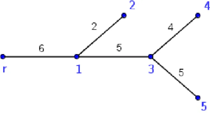
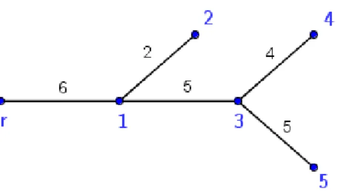
Example 2.5 Figure 2.2 describes a ditch, in which the set of users is N = {1,2,3,4,5}, andc= (6,2,5,4,5)is the cost vector describing the costs associated with the respective segments. The root of the tree is denoted by r, representing the main ditch to which our ditch connects. In this case we get the following results:

ξ^a(c) = 22

5 , 22 5 , 22

5

, and ξ^s(c) = 6

5, 16 5 , 43

15, 103 15 , 118

15

. In the case of the average cost share rule we divided the overall cost sum (22) into 5 equal parts. In the serial cost share case the cost of segment c1 was divided into 5 parts, since it is utilized by all 5 users. The costs of c₂ are covered by the second user alone, while costs of c3 must be divided evenly among users 3, 4, and 5. Costs of

(23)

c₄ are covered by user 4 alone, and similarly, costs of c₅ are covered by user 5.

These partial sums must be added up for all segments associated with each user.

In the following we characterize the above cost allocation rules, and introduce axioms which are expected to be fullled for proper modeling. Comparison of vectors is always done by comparing each coordinate, i.e. c ≤ c⁰, if ∀i ∈ N: c_i ≤c⁰_i.

Axiom 2.6 A rule ξ is cost monotone, if ∀c≤c⁰: ξ(c)≤ξ(c⁰).

Axiom 2.7 A rule ξ satises ranking, if ∀c ∈ R^N+ and ∀j ∀i ∈ I_j⁻ ∪ {j}: ξi(c)≤ξj(c).

Remark 2.8 In the case of chains ξ satises ranking, if ∀i≤j: ξ_i(c)≤ξ_j(c). Axiom 2.9 A rule ξ is subsidy-free, if ∀c∈R^N+ and ∀I ={i₁, i₂, . . . , i_k} ⊆N:

X

j∈J

ξj(c)≤X

j∈J

cj, where for the sake of brevity J := I_i⁻

1 ∪ · · · ∪I_i⁻

k ∪ I, where J is the sub-tree generated by I.

Remark 2.10 In the case of chains setJ will always be the setI_i⁻∪{i}associated with I's highest index member i, i.e. j ∈J if and only if j ≤i. In this case ξ is subsidy-free if ∀i∈N and c∈R^N+:

X

j≤i

ξ_j(c)≤X

j≤i

c_j.

The interpretation of the three axioms is straightforward. Cost monotonicity ensures that in case of increasing costs, the cost of no user shall decrease.

Therefore, no user shall prot from any transaction that increases the overall cost.

If ranking is satised, cost allocations can be ordered by the ratio of ditch usage of each user. In other words, if i∈I_j⁻, then by denition user j utilizes more segments of the ditch than i, i.e. the cost for j is at least as much as for i. The subsidy-free property prevents any group of users having to pay more than the overall cost of the entire group. If this is not satised then some groups

(24)

of users would have to pay for segments they are using, and pay further subsidy for users further down in the system. This would prevent us from achieving our goal of providing a fair cost allocation. (In a properly dened cooperative game, i.e. in irrigation games, the subsidy-free property ensures that core allocation is achieved as a result, see Radványi (2010) (in Hungarian) and Theorem 5.16 of present thesis.)

Furthermore, it may be easily veried that the serial cost allocation rule satises all three axioms, while the average cost allocation rule satises only the rst two (Aadland and Kolpin, 1998).

In the following we introduce two further allocation concepts and examine which axioms they satisfy. These models are based on the work of Solymosi (2007).

Let us introduce the following denitions.

Letc(N)denote the total cost of operations and maintenance of the ditch, i.e.

P

i∈Nc_i. The sum s_i =c(N)−c(N \ {i}) is the separable cost, wherec(N \ {i}) denotes the cost of the maintenance of the ditch, if i is not served. (Note that on the leaves, s_i always equals to c_i, otherwise it's 0.) We seek a cost allocation ξ(c) that satises theξ_i(c)≥s_i inequality for all i∈N. A further open question is how much individual users should cover from the remaining non-separable (or common) cost

k(N) = c(N)−X

i∈N

s_i =c(N)−X

i∈L

c_i.

The users do not utilize the ditch to the same degree, they only require its dierent segments. Therefore, we do not want users to pay more than as if they were using the ditch alone. Let e(i)denote the individual cost of user i∈N:

e(i) = X

j∈I_i⁻∪{i}

c_j.

Fairness, therefore, means that the ξi(c)≤e(i) inequality must be satised for all i∈N. Of course, the aforementioned two conditions can only be met if

c(N)≤c(N \ {i}) +e(i),

for alli∈N. In our case this is always true. By rearranging the inequality we get

− \ {i})≤ , i.e. ≤

(25)

Ifiis not a leaf, then the value ofs_i is 0, while e(i)is trivially non-negative. If i is a leaf, thens_i =c_i, consequentlyc_i ≤e(i)must be satised, as the denition ofe(i)shows. By subtracting the separable costs from the individual costs we get the (k(i) =e(i)−s_i)i∈N vector containing the costs of individual use of common segments.

Based on the above let us consider the below cost allocations:

The non-separable cost's equal allocation:

ξ_i^eq(c) = s_i+ 1

|N|k(N) ∀i∈N

The non-separable cost's allocation based on the ratio of individual use:

ξ_i^riu(c) =si+ k_i P

j∈N

k_jk(N) ∀i∈N

The above dened cost allocation rules are also known in the literature as equal allocation of non-separable costs and alternative cost avoided methods, respectively (Stran and Heaney, 1981).

Example 2.11 Let us consider the ditch in Example 2.5 (Figure 2.2). The previous two allocations can therefore be calculated as follows: c(N) = 22, s = (0,2,0,4,5), k(N) = 11, e = (6,8,11,15,16), and k = (6,6,11,11,11). This means

ξ^eq(c) = 11

5 , 21 5 , 11

5 , 31 5 , 36

5

and

ξ^riu(c) = 66

45, 156 45 , 121

45 , 301 45 , 346

45

.

In the following we examine which axioms these cost allocation rules satisfy.

Let us rst consider the case of even distribution of the non-separable part.

Lemma 2.12 The rule ξ^eq is cost monotone.

Proof: We must show that if c≤c⁰ then ξ^eq(c)≤ξ^eq(c⁰). Vector s(c) comprising separable costs is as follows: for all i ∈ L: s_i = c_i, otherwise 0. Accordingly, we consider two dierent cases, rst when the cost increase is not realized on a leaf,

(26)

and secondly when the cost increases on leaves. In the rst case vectorsdoes not change, but k_c(N)≤k_c⁰(N), since

k_c(N) = c(N)−X

i∈L

c_i,

kc⁰(N) =c⁰(N)−X

i∈L

c⁰_i =c⁰(N)−X

i∈L

ci

and c(N)≤c⁰(N), therefore the claim holds.

However, in the second case for i∈L: s_i(c)≤s_i(c⁰), k_c(N) = X

i∈N\L

c_i = X

i∈N\L

c⁰_i =k_c⁰(N),

hence k(N) does not change, in other words, the value of ξ_n^eq could not have decreased. If these two cases hold at the same time, then there is an increase in both vector s and k(N), therefore their sum could not have decreased, either.

Lemma 2.13 The rule ξ^eq satises ranking.

Proof: We must verify that for any i and j, in case of i ∈ I_j⁻: ξ_iêq(c) ≤ ξ_jêq(c) holds. Since for a xed c in case of ξ_iêq(c) = ξ_hêq ∀i, h ∈I_j⁻, and j ∈ L: ξêq_i < ξ_jêq

∀i∈I_j⁻, the property is satised.

Lemma 2.14 The rule ξ^eq (with cost vector c 6= 0) is not subsidy-free if and only if the tree representing the problem contains a chain with length of at least 3.

Proof: If the tree consists of chains with length of 1, the property is trivially satised, since for all cases ξ_i =c_i.

If the tree comprises chains with length of 2, the property is also satised, since for a given chain we know that:c(N) =c₁+c₂, s= (0, c₂), k(N) = c₁. Therefore ξ₁(c) = 0 +^c₂¹,ξ₂(c) = c₂+^c₂¹, meaning thatξ₁(c)≤c₁ and ξ₁(c) +ξ₂(c)≤c₁+c₂, consequently the allocation is subsidy-free if |N|= 2.

We must mention one more case, when the tree consists of chains with length of at most 2, but these are not independent, but branching. This means that from the rst node two further separate nodes branch out (for 3 nodes this is a

(27)

is satised in these cases as well, since the c₁ cost is further divided into as many parts as the number of connected nodes. Therefore, for chains with length of at most 2, the subsidy-free property is still satised. If this is true for a tree comprising chains of length of at most 2, then the nodes may be chosen in any way, the subsidy-free property will still be satised, since for all associated inequalities we know the property is satised, hence it will hold for the sums of the inequalities, too.

Let us now consider the case when there is a chain with length of 3. Since the property must be satised for all cost structures, it is sucient to give one example when it does not. For a chain with length of at least 3 (if there are more, then for any of them) we can write the following: c(N) =c₁+c₂+· · ·+c_n, s= (0,0,· · ·0, c_n),k(N) = c₁+c₂+· · ·+cn−1. Based on thisξ₁(c) = 0+^c¹^+···+c_n ⁿ⁻¹, meaning that c₁ can be chosen in all cases such that ξ₁(c) ≤ c₁ condition is not met.

Example 2.15 Let us demonstrate the above with a counter-example for a chain of length of 3. In this special case, ξ₁ = ^c¹^+c₃ ², therefore it is sucient to choose a smaller c₁, i.e. c₂ >2c₁. For example, let c= (3,9,1) on the chain, accordingly c(N) = 13, s= (0,0,1), k(N) = 12, therefore ξ^eq(c) = (0 + ¹²₃,0 + ¹²₃,1 + ¹²₃ ) = (4,4,5). Note that the rst user must pay more than its entry fee, and by paying more the user subsidizes other users further down in the system. This shows that the subsidy-free property is not satised, if the tree comprises a chain with length of at least 3.

Let us now consider the allocation based on the ratio of individual use from non-separable costs.

Lemma 2.16 The rule ξ^riu is not cost monotone.

Proof: We present a simple counter-example: let us consider a chain with length of 4, let N ={1,2,3,4}, c= (1,1,3,1), c⁰ = (1,2,3,1). Cost is increased in case of i= 2. Therefore, cost monotonicity is already falsied for the rst coordinates of ξ^riu(c) and ξ^riu(c⁰), since ξ₁^riu(c) = 5

13 = 0.384, and ξ₁^riu(c⁰) = 6

16 = 0.375, accordingly ξ^riu(c)≥ξ^riu(c⁰) does not hold.

(28)

Lemma 2.17 The rule ξ^riu satises ranking.

Proof: We must show that for i∈I_j⁻:ξ_i(c)≤ξ_j(c). Based on the denition:

ξ_i(c) = s_i+ k(i) P

l∈N

k(l)k(N),

ξ_j(c) = s_j + k(j) P

l∈N

k(l)k(N).

We know that for all i ∈ I_j⁻: s_i ≤ s_j, since i ∈ N \L, therefore s_i = 0, while s_j is 0, if j ∈ N \L or c_j, if j ∈ L. We still have to analyze the relationships of k(i) = e(i)−s_i and k(j) = e(j)−s_j. We must show that k(i) ≤ k(j), for all i∈I_j⁻, because in this caseξ_i(c)≤ξ_j(c).

1. i∈I_j⁻,j /∈L

Therefore s_i = s_j = 0 and e(i) ≤ e(j), since e(i) = P

l∈I_i⁻∪{i}

c_l and e(j) = P

l∈I_j⁻∪{j}

c_l, while I_i⁻∪ {i} ⊂I_j⁻∪ {j}, if i∈I_j⁻. Hence, k(i)≤k(j). 2. i∈I_j⁻,j ∈L

This means that 0 =s_i < s_j =c_j. In this case:

k(i) = e(i)−s_i = X

l∈I_i⁻∪{i}

c_l−0 = X

l∈I_i⁻∪{i}

c_l,

k(j) =e(j)−s_j = X

l∈I_j⁻∪{j}

c_l−c_j = X

l∈I_j⁻

c_l.

i=j−1-re k(i) = k(j),

i∈I_j−1⁻ -re k(i)≤k(j).

To summarize, for all cases k(i)≤k(j), proving our lemma.

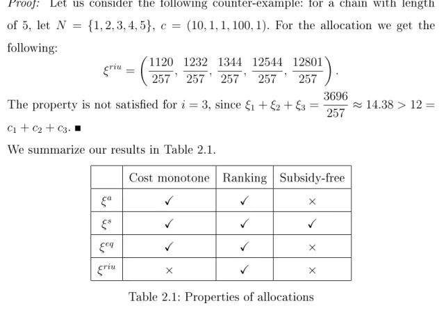
Lemma 2.18 The rule ξ^riu does not satisfy the subsidy-free property for all cases when c∈R⁺.

(29)

Proof: Let us consider the following counter-example: for a chain with length of 5, let N = {1,2,3,4,5}, c = (10,1,1,100,1). For the allocation we get the following:

ξ^riu =

1120 257 , 1232

257 , 1344

257 , 12544

257 , 12801 257

. The property is not satised for i= 3, since ξ₁+ξ₂+ξ₃ = 3696

257 ≈14.38>12 = c₁+c₂+c₃.

We summarize our results in Table 2.1.

Cost monotone Ranking Subsidy-free

ξ^a X X ×

ξ^s X X X

ξ^eq X X ×

ξ^riu × X ×

Table 2.1: Properties of allocations

Based on the above results we shall analyze whether the axioms are independent. The following claim gives an answer to this question.

Claim 2.19 In the case of cost allocation problems represented by tree structures, the properties cost monotonicity, ranking, and subsidy-free are independent of each other.

Let us consider all cases separately:

The subsidy-free property does not depend on the other two properties.

Based on our previous results (see for example Table 2.1), for such cost allocationξ^a is a good example, since it is cost monotone, satises ranking, but is not subsidy-free.

The ranking property is independent of the other two properties. As an example let us consider the allocation known in the literature as Bird's rule. According to this allocation all users pay for the rst segment of the path leading from the root to the user, i.e. ξ_i^Bird =c_i ∀i. It can be shown that this allocation is cost monotone and subsidy-free, but does not satisfy ranking.

(30)

The cost monotone property does not depend on the other two properties. Let us consider the following example with a chain with length of 4, N ={1,2,3,4}, and c={c₁, c₂, c₃, c₄} weights. Let c_m = min{c₁, c₂, c₃, c₄} and c^m = max{c₁, c₂, c₃, c₄}, while C = c^m−c_m. Let us now consider the following cost allocation rule:

ξ_i(c) =







c_m/C, if i6= 4

4

P

i=1

c_i−

3

P

i=1

ξ(c_i) if i= 4.

In other words, user 4 covers the remaining part from the total sum after the rst three users. Trivially, this allocation satises ranking and is subsidy- free. However, with c= (1,2,3,4)and c⁰ = (1,2,3,10) cost vectors (c⁰ ≥c) the allocation is not cost monotone, since if i 6= 4 then ξ_i(c) = 1/3 and ξ_i(c⁰) = 1/9, i.e. ξ_i(c)> ξ_i(c⁰), which contradicts cost monotonicity.

2.2 Restricted average cost allocation

The results of a survey among farmers showed that violating any of the above axioms results in a sense of unfairness (Aadland and Kolpin, 2004). At the same time, we may feel that in the case of serial cost allocation the users further down in the system would in some cases have to pay too much, which may also prevent us from creating a fair allocation. We must harmonize these ndings with the existence of a seemingly average cost allocation. Therefore, we dene a modied rule, which is as close as possible to the average cost allocation rule, and satises all three axioms at the same time. In this section we are generalizing the notions and results of Aadland and Kolpin (1998) from chain to tree.

Denition 2.20 A restricted average cost allocation is a cost monotone, ranking, subsidy-free cost allocation, where the dierence between the highest and lowest distributed costs is the lowest possible, considering all possible allocation prin- ciples.

Naturally, in the case of average cost share the highest and lowest costs are equal. The restricted average cost allocation attempts to make this possible, while

(31)

preserving the expected criteria, in other words, satisfying the axioms. However, the above denition guarantees neither the existence nor the uniqueness of such an allocation. The question of existence is included in the problem of whether dierent cost proles lead to dierent minimization procedures with respect to the dierences in distributed costs. Moreover, uniqueness is an open question too, since the aforementioned minimization does not give direct requirements regarding the internal costs. Theorem 2.21 describes the existence and uniqueness of the restricted average cost share rule.

Let us introduce the following. Let there be given sub-trees H ⊂I and let

P(H, I) = P

j∈I\H

c_j

|I| − |H|·

P (H, I)represents the user costs for theI\H ditch segments, distributed among the associated users.

Theorem 2.21 There exists a restricted average cost share allocation ξ^r and it is unique. The rule can be constructed recursively as follows. Let

µ₁ = min{P (0, J)|J sub-tree}, J₁ = max{J|P(0, J) = µ₁}, µ₂ = min{P (J₁, J)|J₁ ⊂J sub-tree}, J₂ = max{J|P(J₁, J) = µ₂},

... ...

µ_j = min{P (Jj−1, J)|Jj−1 ⊂J sub-tree}, J_j = max{J|P (Jj−1, J) = µ_j},

... ...

and ξ_i^r(c) =µj ∀j = 1, . . . , n⁰, J1 ⊂J2 ⊂. . .⊂Jn⁰ =N, where i∈Jj\Jj−1. The above formula may be interpreted as follows. The value ofµ₁ is the lowest possible among the costs for an individual user, while J1 is the widest sub-tree of ditch segments on which the cost is the lowest possible. The lowest individual user's cost of ditch segments starting fromJ1 isµ2, which is applied to theJ2\J1

subsystem, and so forth.

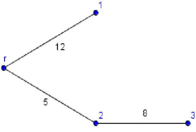
Example 2.22 Let us consider Figure 2.3. In this case the minimum average cost for an individual user is 4, the widest sub-tree on which this is applied is J1 = {1,2}, therefore µ1 = 4. On the remaining sub-tree the minimum average cost for an individual user is 4.5 on the J₂ = {3,4} sub-tree, therefore µ₂ =

(32)

(c3+c4)

2 = 4.5. The remaining c₅ cost applies to J₃ = {5}, i.e. µ₃ = 5. Based on the above ξ^r(c) = (4, 4, 4.5, 4.5, 5).

Figure 2.3: Ditch represented by a tree-structure in Example 2.22 Let us now consider the proof of Theorem 2.21.

Proof: Based on the denition of P(H, I) it is easy to see that ξ^r as given by the above construction does satisfy the basic properties. Let us assume that there exists another ξ that is at least as good with respect to the objective function, i.e. besides ξ^r, ξ also satises the properties. Let us consider a tree and cost vector cfor which ξ provides a dierent result than ξ^r, and let the value ofn⁰ in the construction of ξ^r be minimal. If ξ(c) 6= ξ^r(c), then there exists i for which ξ_i(c) > ξ_i^r(c), among these let us consider the rst (i.e. the rst node with such properties in the xed order of nodes). This is i ∈ Jk\Jk−1, or ξ^r_i(c) = µk. We analyze two cases:

1. k < n⁰:

The construction of ξ^r implies that P

j∈J_kξ^r_j(c) = P

j∈J_kc_j ≥ P

j∈J_kξ_j(c), with the latter inequality a consequence of the subsidy-free property. Since the inequality holds, it follows that there exists h∈J_k, for which ξ_h^r(c)> ξ_h(c).

In addition, let c⁰ < c be as follows: In the case of j ∈ Jk, c⁰_j = cj, while for j /∈J_k it holds thatξ_j^r(c⁰) = µ_k. The latter decrease is a valid step, since in c for all not in Jk the value of ξ_j^r(c) was larger than µk, because of the construction.

Because of cost-monotonicity, the selection of h, and the construction of c⁰, the following holds:

ξ_h(c⁰)≤ξ_h(c)< ξ^r_h(c) = ξ_h^r(c⁰) =µ_k.

(33)

Consequently, ξ_h(c)< ξ_h^r(c), and in the case of c⁰ the construction consist of only k < n⁰ steps, which contradicts that n⁰ is minimal (ifn⁰ = 1then ξ^r equals to the average and is therefore unique).

2. k=n⁰:

In this case ξ_i(c)> ξ_i^r(c) =µ_n⁰, and at the same time ξ₁(c)≤ξ₁^r(c)(since due to k = n⁰ there is no earlier that is greater). Consequently, in the case of ξ the dierence between the distributed minimum and maximum costs is larger than for ξ^r, which contradicts the minimization condition.

By denition the restricted average cost allocation was constructed by minimizing the dierence between the smallest and largest cost, at the same time preserving the cost monotone, ranking and subsidy-free properties. In their article Dutta and Ray (1989) introduce the so called egalitarian allocation, describing a fair allocation in connection with Lorenz-maximization. They have shown that for irrigation problems dened on chains (and irrigation games, which we dene later) the egalitarian allocation is identical to the restricted average cost allocation. Moreover, for convex games the allocation can be uniquely dened using an algorithm similar to the above.

According to our next theorem the same result can be achieved by simply minimizing the largest value calculated as a result of the cost allocation. If we measure usefulness as a negative cost, the problem becomes equivalent to maximizing Rawlsian welfare (according to Rawlsian welfare the increase of society's welfare can be achieved by increasing the welfare of those worst-o). Namely, in our case maximizing Rawlsian welfare is equivalent to minimizing the costs of the nth user. Accordingly, the restricted average cost allocation can be perceived as a collective aspiration towards maximizing societal welfare, on the basis of equity.

Theorem 2.23 The restricted average cost rule is the only cost monotone, ranking, subsidy-free method providing maximal Rawlsian welfare.

Proof: The proof is analogous to that of Theorem 2.21. The ξ_i(c)> ξ_i^r(c) = µ_n⁰ result in the last step of the aforementioned proof also means that in the case of ξ allocation Rawlsian welfare cannot be maximal, leading to a contradiction.

In the following we discuss an additional property of the restricted average cost rule, which helps expressing fairness of cost allocations in a more subtle

(34)

way. We introduce an axiom that enforces a group of users that has so far been subsidized to partake in paying for increased total costs, should such an increase be introduced in the system. This axiom and Theorem 2.25 as shown by Aadland and Kolpin (1998) are as follows:

Axiom 2.24 A rule ξ satises the reciprocity axiom, if ∀i the points (a) P

h≤iξ_h(c)≤P

h≤ic_h (b) c⁰ ≥c and

(c) P

h≤i(c_h−ξ_h(c))≥P

j>i(c⁰_j −c_j)

imply that the following is not true: ξ_h(c⁰)−ξ_h(c) < ξ_j(c⁰)−ξ_j(c) ∀h ≤ i and j > i.

The reciprocity axiom describes that if (a) users{1, ..., i}receive (even a small) subsidy, (b) costs increase from c to c⁰, and (c) in case the additional costs are higher on the segments afteri than the subsidy received by group{1, ..., i}, then it would be inequitable if the members of the subsidized group had to incur less additional cost than the {i+ 1, ..., n} segment subsidizing them. Intuitively, as long as the cost increase of users {i+ 1, ..., n} is no greater than the subsidy given to users {1, ..., i}, the subsidized group is indebted towards the subsidizing group (even if only to a small degree). The reciprocity axiom ensures that for at least one member of the subsidizing group the cost increase is no greater than the highest cost increase in the subsidized group.

Theorem 2.25 (Aadland and Kolpin, 1998) The restricted average cost allocation, when applied to chains meets cost monotonicity, ranking, subsidy-free and reciprocity.

2.3 Additional properties of serial cost allocation

The serial cost allocation rule is also of high importance with respect to our original problem statement. In this section we present further properties of this allocation. The axioms and theorems are based on the article of Aadland and Kolpin (1998).

(35)

Axiom 2.26 A rule ξ is semi-marginal, if ∀i ∈ N \L: ξ_i+1(c) ≤ ξ_i(c) +c_i+1, where i+ 1 denotes a direct successor of i in I_i⁺.

Axiom 2.27 A rule ξ is incremental subsidy-free, if ∀i∈N and c≤c⁰: X

h∈I_i⁻∪{i}

(ξh(c⁰)−ξh(c))≤ X

h∈I_i⁻∪{i}

(c⁰_h−ch).

Semi-marginality expresses that if ξ_i(c) is a fair allocation onI_i⁻∪ {i}, then user i+ 1 must not pay more than ξ_i(c) +c_i+1. Increasing subsidy-free ensures that starting fromξ(c)in case of a cost increase no group of users shall pay more than the total additional cost.

For sake of completeness we note that increasing subsidy-free does not imply subsidy-free as dened earlier (see Axiom 2.9). We demonstrate this with the following counter-example.

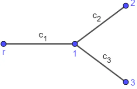
Example 2.28 Let us consider an example with 3 users, and dened by the cost vector c= (c₁, c₂, c₃) and Figure 2.4.

Figure 2.4: Tree structure in Example 2.28

Let the cost allocation in question be the following:ξ(c) = (0, c₂−1, c₁+c₃+1). This allocation is incremental subsidy-free with arbitrary c⁰ = (c⁰₁, c⁰₂, c⁰₃), given that c≤c⁰. This can be demonstrated with a simple calculation: