INTERNATIONAL ECONOMICS LECTURE NOTES
This note is based on
Gyula Bock, György Martin Hajdu, András Réz, Ferenc Tóth (1991):
Nemzatközi gazdaságtan, Bíbor Kiadó, Miskolc
Nedelka Erzsébet
SOPRONI EGYETEM
LÁMFALUSSY SÁNDOR KÖZGAZDASÁGTUDOMÁNYI KAR Sopron 2019
Jelen tananyag az „EFOP-3.4.3-16-2016-00022„QUALITAS” Minőségi felsőoktatás fejlesztés Sopronban, Szombathelyen és Tatán” projekt keretén belül jött létre.
This note was supported by EFOP-3.4.3-16-2016-00022 „QUALITAS”
Minőségi felsőoktatás fejlesztés Sopronban, Szombathelyen, és Tatán project
Nedelka Erzsébet a Nyugat-magyarországi Egyetem Közgazdaságtudományi Karán végzett okleveles közgazdászkén, majd az egyetem falain belül maradva, megkezdte a doktori képzést nappalis doktoranduszként a Széchényi István Gazdálkodás- és Szervezéstudományi Doktori Iskolában. 2018-ban szerzett fokozatot. Öt éve tanít az azóta már Soproni Egyetem Lámfalussy Sándor Közgazdaságtudományi Karként ismert felsőoktatási intézményben.
Fő területe a nemzetközi gazdaságtan, az Európai Uniós ismeretek, nemzetközi gazdasági elemzések, az interkulturális menedzsment és kommunikáció.
Erzsébet Nedelka graduated at University of West Hungary Faculty of Economics in 2010 but she remained at the University and started a PhD course in Management and Organisational Sciences. She defended successfully her thesis in 2018. For 5 years she has been teaching international economics, European studies, international economic analysis, intercultural management and communication at University of Sopron, Alexandre Lamfalussy Faculty of Economics.
Table of contents
1. The theory of absolute and comparative advantages ... 1
1.1 Adam Smith and absolute advantages ... 2
1.2 David Ricardo and Comparative advantages ... 5
1.3 Specialization and foreign trade in case of constant opportunity cost ... 6
1.4 World transformation/production curve in case of constant opportunity costs ... 8
1.5 Specialization and foreign trade in case of increasing opportunity cost... 9
1.6 World transformation/production curve in case of increasing opportunity costs .11 1.7 Specialization and foreign trade in case of increasing opportunity cost from the Aspect of Ricardo’s comparative advantages ...12
2. The effect of production conditions on foreign trade ...14
2.1 Production function and transformation curve in the case of constant returns to scale 14 2.1.1 Edgeworth-box and transformation curve ...17
2.2 Non-linear production function – increasing and decreasing returns to scale ...19
2.3 Heckscher-Ohlin Hypothesis – Heckscher-Ohlin model...20
2.3.1 Leontief-paradox ...22
2.4 Factor price equalization ...23
2.4.1 Equalization of factor prices in the real economy ...27
3. Demand, terms of trade and general equilibrium in international trade ...29
3.1 Demand in the model ...29
3.1.1 Effect of trade and specialization on social utility in case of constant opportunity cost...30
3.1.2 Effect of trade and specialization on social utility in case of increasing opportunity cost... -32
3.1.3 Effect of trade and specialization on social utility in case of different consumer preferences ...35
3.2 Offer curve and international terms of trade ...36
3.2.1 Disequilibrium and equilibrium – Restoring balance ...38
3.2.2 Different offer curves in international trade ...40
3.3 Trade indifference curve ...41
3.3.1 Offer curve and trade indifference curve ...42
3.4 Meade’s General equilibrium model ...44
4. Protectionism ...45
4.1 Customs ...46
4.1.1 Overview of customs ...46
4.1.2 Carrying the burdens of customs ...48
4.2 Effect of customs on domestic market ...51
4.3 Effect of Quotas on domestic market ...53
List of Figures
1. Figure: Production possibility frontier/transformation curve/production curve ... 4
2. Figure. Specialization and foreign trade in case of constant opportunity cost. ... 6
3. Figure. World tranformation curve – Constatnt opportunity costs ... 9
4. Figure. Specialization and foreign trade in case of increasing opportunity costs. ...10
5. Figure. World transofrmation curve – Increasing opportunity costs ...11
6. Figure. Ricardo’s comparativ advantages ...13
7. Figure. Lack of comparative advantages and disadvantages ...13
8. Figure. Conditions of production for two products...15
9. Figure. Edgeworth-box ...17
10. Figure. Transformation curve derived from Edgeworth-boksz ...18
11. Figure. The shape of contract curve. ...18
12. Figure. Hechscher-Ohlin model ...21
13. Figure. Equalization of price ratio of factors of production...25
14. Figure. Cost of labour within the European Union in 2018 ...28
15. Figure. Socail indifference curve in case of constant opportunity costs – world model ..31
16. Figure. Social indifference curve in case of increasing opportunity costs ...32
17. Figure. Socail indifference curve in case of increasing opportunity costs – world model ...33
18. Figure. Advantages of foreign trade without specialization ...35
19. Figure. Trade and specialization in case of different consumer preferences ...36
20. Figure. Offer curve ...37
21. Figure. Restoring equilibrium ...39
22. Figure. International terms of trade, export-import and different consumer preferences 40 23. Figure. Trade indifference curve derived from social indifference curve ...42
24. Figure. Explanation of trade indifference curve ...42
25. Figure. Offer curve derived from trade indifference curve ...43
26. Figure. Meade’s General Equilibrium Model of ...44
27. Figure. Equal distribution of burden of customs ...48
28. Figure. Unequal distribution of burden of customs ...50
29. Figure. Internal/domestic effect of customs ...52
30. Figure. Internal/domestic effects of quotas ...54
List of abbreviations d – deadweight loss EX (or X) – export G – offer curve IM – import
J – social indifference curve K – capital
L – labour
MP – marginal product
MRS – marginal rate of substitution MRT – marginal rate of transportation MU – marginal utility
PD – the price ratio of demand px – price of X product
py – price of Y product
T – trade indifference curve and customs/tariffs
1
PREFACE
The aim of this note was to give an overview about the theory of international economics to our students. Of course, there are many good books in English about this topic, but most of them do not fit to our requirements or they are too complex, and we do not have enough time. Therefore, we decided to use a Hungarian book in the English language course as well which was written in 1991 but still one of the best about the main theories of international economics. In order to help foreign student, beside of our presentations, we give written explanation to models we made this note for. Most of the figures are from the above-mentioned book and our explanations and comments are also based on it. Therefore, we do not refer the book in every case. Just at the cover page and after figures.
We hope this note helps students to learn those theories of international economics which are essential to an economist. To better understand models, you should use videos available on our e-learning portal. Videos contain animated models with narrations.
2
1. THE THEORY OF ABSOLUTE AND COMPARATIVE ADVANTAGES
1.1 ADAM SMITH AND ABSOLUTE ADVANTAGES
Adam Smith was a Scottish economist and philosopher who was born in 1723. During his working years, the economy was in the age of colonial type international division of labour. The main features of this age were the well- organized foreign traded and financial processes. The emperors exploited their colonies and wanted to increase the volume of export in order to get more and more surplus from international trade. Beside of the increasing volume of foreign trade, economies got another impulse. This impulse was the first industrial revolution. Finally, this is the age of classical capitalism and Adam Smith was the one who posed its principles.
In this period, the condition of production varied or was different from country to country. Based on differences countries shared their production and produced only those products in which they had absolute advantages compared to the other countries. This was and still is the main principle of division of labour. (However, in Adam Smith’s time this concept was not used, Emile Durkheim was the one who used this phrase but in another sense). According to Adam Smith, countries trade with each other because they are different from each other and want to achieve economies of scale in production. If each country produces only a limited range of goods, it can produce each of these goods at a larger scale and hence more efficiently than if it tries to produce everything by itself. Nowadays, this kind of trade appears among brands and less among different types of goods. In order to be able to explain absolute advantages, we have to pose some conditions. In this model, we have two countries (I and II), two products (X and Y) and only one factor of production
3 which is labour. The two countries have different production conditions. If the I. country can produce X products on a lower cost per unit, while the II. country can produce Y products on a lower cost per unit, than I. country has absolute advantage in the X production and II. country has absolute advantage in the Y production. Therefore, first country has to give up the production of Y products (even one unit of Y product is not efficient, but in our models efficiency is important), second country has to give up the production of X products, so first country will produce only X products, while second country will produce only Y products after they finished the specialization.
We can explain the process with functions as well, but first some phrases have to be clear up:
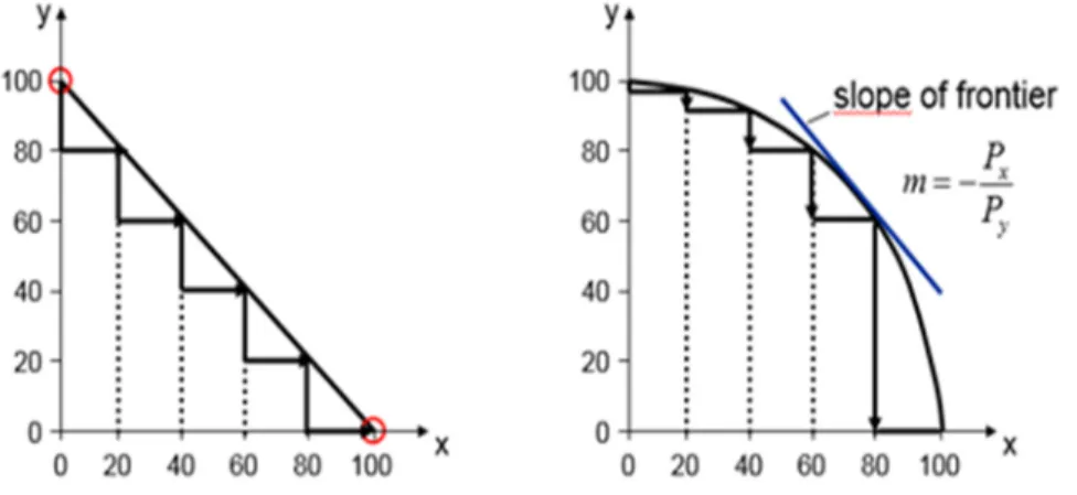
production curve/production possibility frontier: the curve represents graphically alternative production possibilities between two products when there is a fixed amount or availability of resources. The curve represents the point at which an economy is the most efficient.
linear production curve: opportunity costs are constant
bulging downward curve: opportunity costs are increasing
opportunity cost (alternative): the cost of choosing between alternatives, it represents the benefit an economy missed out on when choosing one alternative over another.
First figure represents the constant; the second figure represents the increasing opportunity cost. In case of linear transformation curve, you always have to give up the same number of Y products in order to produce one unit of additional X product. According to the figure, you have to give up 20 Y products in order to produce additional 20 X products. Which means that in this example the opportunity cost is 1. If you have increasing opportunity cost, you have to give up a greater number of Y products in order to produce one
4 unit of addition X product. According to the figure, you have to give up approx.
5 Y in order to get 20 X, but if you want to get 20 more X you have to give up 10 more Y and so on.
1. Figure: Production possibility frontier/transformation curve/production curve
Source: Bock et. al., 1991.
The reason for increasing alternative cost can be the specific factors of production. At the first phase of specialization, countries redistribute easily mobilizable factors but after we finished their redistribution we should mobilize our specific factors as well, but we cannot reach as much output as before or better to say our losses will increase. Determination of opportunity cost is not as easy an in case of linear production curve. We have to introduce a new phase, which is the marginal rate of transformation (MRT). Marginal rate of transformation shows that how many units of one product have to be reduced in order to increase the production of the other product at a given point of production curve. Marginal rate of transformation is equal with alternative cost:
marginal alternative cost of X product:
marginal alternative cots of Y product:
5 1.2 DAVID RICARDO AND COMPARATIVE ADVANTAGES
David Ricardo developed or better to say published this theory in 1817.
Comparative advantages theory offered a solution for a problem that arose after Adam Smith introduced absolute advantages. The problem was that many countries traded with each other despite of the fact that one of them can produce every single good more efficient than the other one, so according to Smith’s theory there was no reason for their trade. David Ricardo discovered that the answer is in their opportunity costs. Until the opportunity cost is not the same in two countries, they have reason for trade. A classic example is Portugal wine and English cloth. Portugal has absolute advantage in wine and cloth production as well, but in a different scale. As you can see in the first table, 1.5 times more working hour required UK to produce one unit of wine and 1.1 times more working hour for cloth. With other words, Portugal needs fewer working hour for production of wine and cloth; it can produce more products during the same period. According to Ricardo’s theory, there is still opportunity for trade. Because of the difference is larger in case of wine than cloth therefore, Portugal should specialize for wine and United Kingdom should specialize for cloth. United Kingdom has namely comparative advantages in cloth and comparative disadvantages in wine, while Portugal has comparative advantages in wine and disadvantages in cloth.
1. Table: Example for Ricardo’s comparative advantages
working hour required wine – one unit cloth – one unit
Portugal 80 90
United Kingdom 120 100
12080 1,5 100 90 1,11
Source: Bock et. al., 1991
6 The existence of comparative advantages does not mean that countries can or want to utilize them. Really good example for this is when countries have to face with some trade barriers like quotas, customs or any other similar restrictions. But if we do not have to struggle with any kind of trade barriers, in a perfect market, market mechanisms lead to the redistribution of production factors, so specialization. Ricardo’s theory gives also explanation how mutually beneficial trade can be between or among countries with different level of development.
1.3 SPECIALIZATION AND FOREIGN TRADE IN CASE OF CONSTANT OPPORTUNITY COST
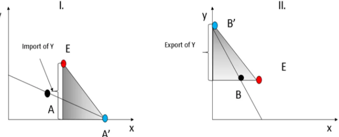
Assuming that there are two countries, which start to trade with each other, and both of them have constant opportunity cost (PPF line is linear) we can draw the following model:
2. Figure. Specialization and foreign trade in case of constant opportunity cost.
Source: Bock et. al., 1991.
7 I. country has better conditions in the production of X product; the opportunity cost of one X product is approx. ⅓ Y products. From the aspect of Y product, its opportunity cost is three X products. So, the inner terms of trade before foreign trade: 1 X = ⅓ Y in the I. country.
In the second country, we can see the opposite. II. country has better conditions in the production of Y product, the opportunity cost of one Y product is approx. ⅓ X product, from the aspect of X product, its opportunity cost is 3Y products. So, the inner terms of trade before foreign trade: 1 X = 3Y.
For the II. country is better to import X product from I. country and should specialize only for Y product and export it to the I. country. For the I.
country is better to import Y product from II. country and should specialize only for X product and sell it to the II. county. On the 2nd figure A and B points represent the autarch (before trade) production and consumption point.
Production and consumption point must be the same in case of self-sufficiency because citizens can consume as much as their economy produces. After the two countries start to trade with each other and change their economic structure (so starts to specialize), production point and consumption point will not have to be the same. Because of constant opportunity cost, specialization is absolutely complete, the new production points are A’ and B’ and the new consumption point is E. If we project these points to X and Y axes, we can get a triangle in each country. This triangle is the foreign trade triangle. One leg/cathetus represents export, the other one represents import.
After these two countries started to trade with each other and finished specialization the new terms of trade in both country (according to our example) is 1X = 1Y. In our model only these two countries are, therefore, the international terms of trade is equal with theirs. If international terms of trade is among the self-supporting terms of trade both country can enjoy the advantages of foreign trade. Consumption point is the part of consumption line
8 which slope also represents the terms of trade not just the national but also international terms of trade.
1.4 WORLD TRANSFORMATION/PRODUCTION CURVE IN CASE OF CONSTANT OPPORTUNITY COSTS
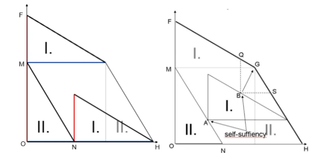
In order to be able to demonstrate the advantages of specialization from production side, production aspect, we need to adopt a new means, the world transformation curve/world production possibility frontier. The model of world usually contains two countries, but there are opportunities to make models which deduce the world transformation curve of more countries. World transformation curve or production possibility frontier represents the total amount of products, which can be produced with available input within the world. The figure represents this curve if opportunity cost is constant and if there are just 2 countries in the world. The area marked with I. represents the set of first country’s production opportunities (production block). The area marked with II. represents the production block of second country. Hypotenuse of triangles gives world production possibility frontier (FG + GH). The maximum production of Y product is represented by OF stage, while the maximum production of X product is represented by OH stage. OM and ON stages are produced by II. country, MF and NH stages are produced by I.
country. Until the two countries do not trade with each other and do not specialize their economies the inner production and consumption points are A and B, and these two points give together the world production point in autarchy. B point is under the world’s production possibility frontier therefore it is suboptimal. After countries transform the structure of their economies and finish specialization (which based on absolute or at least comparative advantages) world production point moves from B to G point and gets to the FH stage, which represents optimal level. According to absolute (and
9 comparative) advantages, specialization increases the efficiency of production which can lead to increasing welfare as well. In a later chapter we explain this process in detail.
3. Figure. World tranformation curve – Constatnt opportunity costs Source: Bock et. al., 1991.
1.5 SPECIALIZATION AND FOREIGN TRADE IN CASE OF INCREASING OPPORTUNITY COST
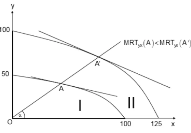
If we suppose that opportunity cost is increasing in both countries, then production possibility frontier is concave to origin therefore, the determination of price ration (slope of the curve) is a bit more difficult because in each point the slope is different. The specialization will not be complete. The difference between marginal rates of transformation depends not only on different production conditions but also on differences in demand factors, but it is not important for us now. The trading and specialization process is quite the same, but now as we have already mentioned, specialization cannot be complete therefore A’ and B’ points are not on axes. So, first country still produces Y product (after specialization) and second country produces X product but of course less. In self-sufficiency, MRT is ¼ in I. country and 4 in II. country. If
10 MRT is different countries have opportunity to trade with each other and specialize their economies to produce X or Y product.
4. Figure. Specialization and foreign trade in case of increasing opportunity costs.
Source: Bock et. al., 1991.
After specialization, following equation must be fulfilled:
The opportunity of free international trade consolidates internal terms of trade in both countries because they increase trade volume until the utilization of international price differences makes extra-profit possible.
Moreover, in order to fulfil one of the main principles of perfect market, so prices stay equal with the marginal cost, the factors of production must be relocated. Consequently, the impact of market forces results in the changes of production points (from A to A’ and from B to B’). In the new points, we can say that countries absolutely utilized the potential advantages of the originally different price ratio.
11 If we further assume that the new consumption points will be in E point, than we can draw again a foreign trade triangle. One cathetus represents export volume that is equal with the other one that represents import volume
1.6 WORLD TRANSFORMATION/PRODUCTION CURVE IN CASE OF INCREASING OPPORTUNITY COSTS
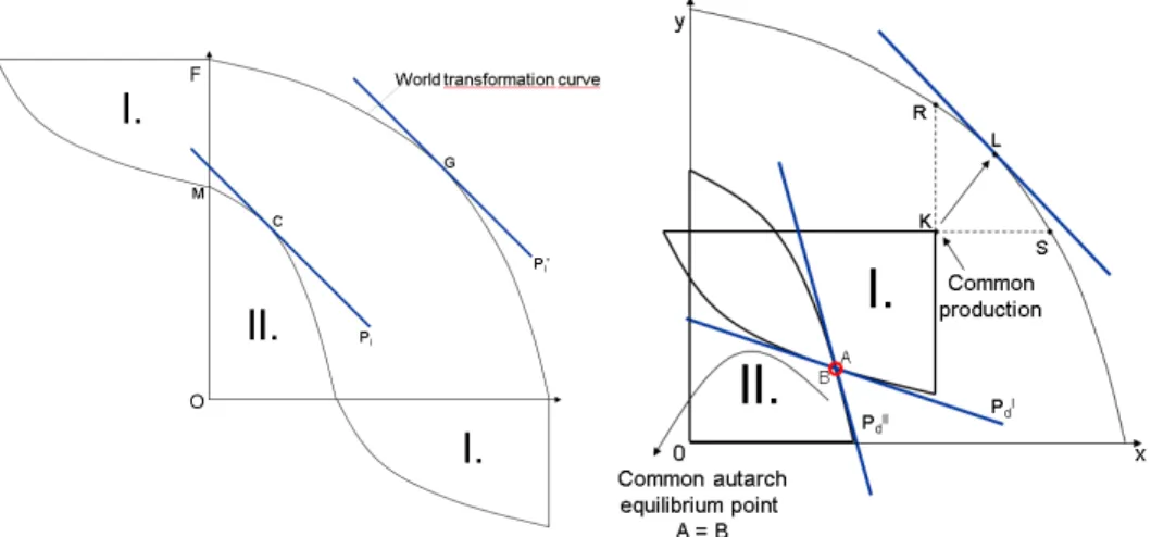
Editing a world transformation curve when we have increasing opportunity cost is a little bit more difficult because of the concave nature of production possibility frontiers. We cannot just simply put the first production block on the second one. The figure represents how we can get it.
5. Figure. World transofrmation curve – Increasing opportunity costs Source: Bock et. al., 1991.
As you can see in the figure, now we have to fit the two production blocks based on their self-supporting production and consumption point together (so A and B point have to be on each other). K point will represent the production and consumption point of world before foreign trade and specialization. The process is quite similar to constant opportunity cost; the
12 only main difference is that specialization will not be complete. But both countries change their production structure, specialize for X or Y products, therefore the efficiency of their economies will increase, and they will be able to reach world production possibility frontier together. If the specialization happens similarly, the production and consumption point will move from K (suboptimal point) to L point. During the period of self-sufficiency, the slope of and line represents inner price ratios, after foreign trade and specialization we can draw a tangent on L point. The slope of this tangent shows us new price ratio. This price ratio is for the first and second country, and for world, too. Provision of specialization which improves the efficiency
of world-wide production is: ≠ .
1.7 SPECIALIZATION AND FOREIGN TRADE IN CASE OF INCREASING OPPORTUNITY COST FROM THE ASPECT OF RICARDO’S COMPARATIVE ADVANTAGES
Our previous examples were based on clear advantages and disadvantages, so they were better examples for Adam Smith’s theory. Now let us see the case of Ricardo’s comparative advantages; what happens if we do not have comparative advantages and disadvantages. Both countries can produce more X products than Y, but II. country can produce twice as much Y products than I. country but only 1.25th more X products. Which means that first country has comparative advantage in X products, while second country has comparative advantage in Y products. For any value of α following
inequality must be true: < .
13 6. Figure. Ricardo’s comparativ advantages
Source: Bock et. al., 1991.
Our next figure gives an example for a case when we cannot find comparative advantage or disadvantage between two countries. First country can produce less X and Y products. Second country owns absolute advantages in the production of X and Y products. From X products it can produce twice as much, and from Y products, too. So, the main provision of comparative
advantage is not met because the .
7. Figure. Lack of comparative advantages and disadvantages Source: Bock et. al., 1991.
14
2. THE EFFECT OF PRODUCTION CONDITIONS ON FOREIGN TRADE
In previous chapter, we just used one factor of production, which was the labour. But even in the 18th century there was another factor of production which very important part of economy in the 19th century, this was the capital.
Capital means not only money capital but also fixed assets, machines, buildings, any equipment that is used in production. Some countries have more labour and less capital, some countries have more capital and less labour, this fact contributes to the creation of specialization possibility. Moreover, some products require more labour and less capital, while other product requires less labour and more capital. In this chapter, we examine trade and production based on two factors of production.
2.1 PRODUCTION FUNCTION AND TRANSFORMATION CURVE IN THE CASE OF CONSTANT RETURNS TO SCALE
Before we introduce our model, we need to pose some provisos. Firstly, both products are produced with constant returns to scale, which means that we have linearly homogeneous production function. (Main feature of this kind of function is that, if we increase the two factors of production with 1-1%, the volume of production increase with 1%, too. Secondly, one of the products (in our model X product) is capital-intensive, the other one is labour-intensive.
Thirdly, if we exclude the reversal of factor demand the isoquants of X and Y products intersect each other only once. Fourthly, we know the factor endowments of both countries.
15 8. Figure. Conditions of production for two products
Source: Bock et. al., 1991.
The figure represents two products, which requires capital and labour. Y product needs more capital, while X product needs more labour. In this economy, the maximum amount of Y product is 50 unit and in case of X product is 100 unit. Red lines show isocost line and we know from our microeconomic studies, that optimal combination of products are those points where an isocost line and isoquant curve meet with each other. (Isocost line shows those combinations of inputs which cost is the same; isoquant curve represents all factors (the quantities of factors change) which produce the same quantity of output).
In our models, we usually work with two countries, two products and two factors of production; therefore, we need a new tool to visualize it. This new tool is the Edgeworth-box, which can introduce two products and two factors in the same figure. The lower left-hand corner represents the origin for X products, while the upper right-hand corner represents the origin for Y products. From other aspect, the lower left-hand corner is equal with the maximum quantity of Y products, and the upper right-hand corner with the
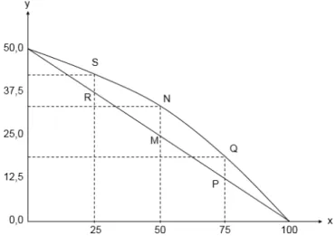
16 maximum quantity of X products. In O point there is no Y production only X is produced (100 units) and in O’ point there is no X production only Y is produced (50 units). The diagonal represents those points where the factors of production are similar for X and Y products, too. The other problem with the diagonal is that isoquant curves (indifference curves) meet with each other twice on this level. Which is suboptimal, we would be able to increase the production of X or Y product. Furthermore, we know that X is labour- intensive, and Y is capital intensive, so diagonal cannot be right. Therefore, we need to make a small correction in order to fit our own provisions and previous figure. So S, N, Q points will represent those ones where an X and Y isoquant are just tangential to each other. Let’s see the S point. In this point an X isoquant which level represents 25 units tangential to an Y isoquant which level is 37.5. In N point, an X isoquant which level shows 50 units tangential to a Y isoquant which level is 25. What happened? We just redistributed our factors of production and so we were able to produce more X products but less Y products. If we connect O-S-N-Q-O’ points, we get the contract curve.
According to the Dictionary of Economics “the contract curve is a set of tangency points between the indifference curves of the two consumers” (in our example between two products). “The competitive equilibrium of an economy is always located on the contract curve”. On the contract curve the provision of efficient production (for X and Y, too) is satisfied:
where MRTS is the marginal rate of technical substitution1.
1 "The rate at which one factor can be substituted for another while holding the level of output constant" (Economicsconcepts.com, 2019).
17 9. Figure. Edgeworth-box
Source: Bock et. al., 1991.
2.1.1 Edgeworth-box and transformation curve
Each point of contract curve can be assigned to each point of transformation curve, if at any point in the contract curve isoquants of X and Y product (x1 and y1) are tangential, then (x1, y1) point lies on the transformation curve as well in the output area. The point of intersection of transformation curve with axes depends on the quantity of factors of production available in a country, productivity, which is represented by isoquants, and finally yet importantly factor intensity of products.
As we saw in the 10th Figure, RMP points can be contract curve if factor intensity of both products is the same. But one of our product (X) is labour- intensive while the other one (Y) is capital-intensive, therefore the shape of our contract curve is convex and because of the increasing opportunity cost transformation curve is concave. If X product was capital-intensive and Y
18 product labour-intensive, the shape of contract curve would be convex, but transformation curve would be still concave (opportunity cost is increasing!).
10. Figure. Transformation curve derived from Edgeworth-boksz Source: Bock et. al., 1991.
The other factor, which influences the shape of contract line and transformation curve, is the differences between factor intensity. The larger the differences of factor intensity, the farther the curve gets from diagonal (it bends stronger). The shape of transformation curve also depends on factor substitution as well. If the opportunity of factor substitution is low, the curve gets further from diagonal, if it is high, then the curve gets closer to diagonal.
A B C D
Source: own edition
11. Figure. The shape of contract curve.
A – x (L), y (K) → convex; B – x (K), y (L) → concave; C – better subsitution of factors; D – weaker substitution of factors
19 2.2 NON-LINEAR PRODUCTION FUNCTION – INCREASING AND DECREASING
RETURNS TO SCALE
Decreasing returns to scale means when we increase our factors in the production, but we still get less than proportional increase in output. With an example, we increase both labour and capital with 1% but the output increase only with 0.8%. Increasing returns to scale means that if we increase our factors in the production, we get more than proportional increase in output.
If we suppose that returns to scale can be increasing or decreasing, and we do not insist on different factor intensity, then we can get many other models from which we just mention four:
1. If the returns to scale of X product is decreasing while for Y product is not increasing, we still get concave transformation curve, but in this case the factor intensity of both products has to be the same.
2. If the returns to scale of X product is increasing while for Y product is not decreasing, then we get convex transformation curve supposing similar factor intensity of products.
3. The situation is a little bit more difficult if we suppose that the returns to scale are increasing and the factor intensities are different, because the first case results in convex and the second in concave transformation curve. If there is only a slight increase in returns of scale then transformation curve is convex closer to axes, but farther from them it is concave.
4. Transformation curve has at least one point of inflexion if returns to scale is increasing in one line of production and decreasing in the other one.
20 2.3 HECKSCHER-OHLIN HYPOTHESIS –HECKSCHER-OHLIN MODEL
Eli Heckscher (1897-1952) was a Swedish political economist and economic historian, Bertil Ohlin (1899-1979) was his student, also Swedish economist and politician. They worked out their theory in the first part of the 20th century, in which they attributed comparative advantages and disadvantages to countries’ different factor endowments. As with all models so far, we have to set again some provisos:
we have two products,
we have two factor of production – labour and capital,
one of the products is labour intensive, the other one is capital intensive,
products and factors of production are homogeneous,
there are not absolute advantages and disadvantages,
production functions are linearly homogeneous → both products are produced with constant returns to scale,
the countries’ factor endowments are different → the ratio of capital and labour is not the same in the two countries → one country is labour abundant, the other is capital abundant.
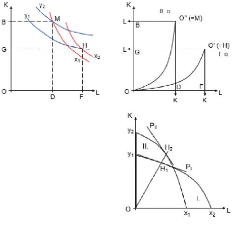
The first part of the 12th Figure represents and verifies the homogeneity of production function in both countries because isoquant of X and Y products related to the first and the second country as well. We can see that the factor- intensity of X and Y products is different, X products are labour intensive, while Y products are capital-intensive. The maximum amount of labour is equal with ⃗ in the first country and the maximum amount of capital is ⃗, in the second country there is ⃗ labour and ⃗ capital. The different factor endowments are really striking at the second part of the 12th Figure which
21 represents two Edgeworth boxes. The vertical one belongs to second country which is capital abundant, the horizontal one belongs to first country which is labour abundant. Third part of 12th Figure shows the transformation curve of two countries.
12. Figure. Hechscher-Ohlin model Source: Bock et. al., 1991.
How can we interpret these coordinate systems? The first two help us to verify and visualize our conditions, while the third explains the essence of Heckscher- Ohlin Model. Labour abundant country has comparative advantages in the production of labour-intensive products, while capital abundant country has comparative advantages in the production of capital-intensive products. ”⃗ is the contract curve of the first country, ⃗ is the contract curve of the second
22 country; O’ and O’’ shows how much X product can be produced, this is the maximum amount of X; while O shows how much Y product can be produced, this is the maximum amount of Y. 3rd part of the figure shows two transformation curves. If we draw a line from O to the transformation curves, we get two intersections. Now we can determine (in these intersections) the slopes of curves. According to our figure following inequality is true in the H1
and H2 < . Each economy produces with comparative advantages those products, which utilize intensively the relatively abundant factor in a given country. Products, which are produced with comparative advantage, is presented with a higher rate within the economy compared to the other country, and excluding extreme demand, these products are exported.
2.3.1 Leontief-paradox
Wassily Leontief (1906-1999) was a Russian-American economist who tested the Heckscher-Ohlin theory on the American economy, and he found that the USA is a capital-abundant country, actually it is the most one in the world, and still exports more labour-intensive products than capital- intensive. Meanwhile in the completely western world the H-O theory has become generally accepted and was regarded as an explanation for foreign/
international trade. Therefore, Leontief’s examination undermined the validity of the Heckscher-Ohlin theory. A quite huge debate started in which statistical methods and other countries were involved as well. These analyses had different results and we still cannot say that the debate is closed. But let us see some explanation for Leontief-paradox. H-O theory supposes that the free flow of products but in that time, USA restricted considerably the import of labour- intensive products. Custom duties and measures having equivalent effect to customs duties distorted the factor-intensity of sector competing with import.
23 Further problem connected to the turning over of factor-intensity, which was excluded by H-O theory. But this phenomenon existed and still exists. The situation is quite similar with international movements of factors of production.
Most models do not take care for them or exclude them, but it was and still is also an existing phenomenon. Many American companies operating out of the USA exported into the mother country and these kind of export products were definitely capital-intensive. If we count them as part of the American economy, it changes the factor-intensity counted by Leontief. (Check what the difference is between GDP and GNI, later you can read about this in details).
Furthermore, we can separate labour for two part as well, and one of them is highly qualified, which is called therefore nowadays as human capital.
American export requires not just simple labour but highly qualified one while the import-substituting sectors or sectors, which compete with import, use relative more unqualified labour force. So if we regarded the highly qualified labour force as capital, then the American export fits to the H-O theory and capital intensive.
This differentiation of factor of production still fits to the H-O theory, but some trade models were born after the H-O theory, which handled the concept of factor of production quite flexible and counted with 15 or even with more than 20 factors. These models are the so-called neo-factor theories and regard the cost of R&D, marketing, logistics and even increasing returns to scale as factors of production. Their aim is not just to explain comparative advantages and disadvantages, but they also make a proposal how to implement them.
2.4 FACTOR PRICE EQUALIZATION
The theory of factor price equalization delivered from H-O theory. If we suppose the free movement of factors, their prices, or better to say, their
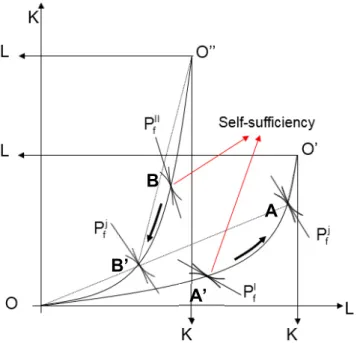
24 price ratio is equalised. What does it mean? It is not necessary that two country have the same prices but the ratio of two factor like capital/labour should be the same. (If we remain on the level of products not on factors, you can buy as much bread or milk from your money in Hungary where the Forint is the national currency as in Slovakia where the Euro is the national currency, or in Germany – this is what the equilibrium of price ratio means). The 12th Figure represents its process. We can see two Edgeworth-box. The horizontal shows the second country, while the vertical shows the first country. Second country is relatively capital abundant, first country is relatively labour abundant. O point represents the maximum amount of Y products, O’ and O” represents the maximum amount of X products. A and B point show the production in self- sufficiency. In self-sufficiency, the capital is relatively expensive to labour in the first country, while the labour is relatively cheap. In the second country the opposite is true. Therefore, supplying the demand for Y products (capital- intensive) is hard for the economy in the first country and burdensome capital.
On the other side we have a product which is labour-intensive one but because the abundance of labour forces this factor of production is not so burdensome, and demand is not as intensive as in case of the capital-intensive product. In the second country, everything is contrary.
As you can see in point A and B there are two isoquants which are tangential to each other. The slope of their tangents ( and ) also represents the difference of price ratio of factors. After these two countries start to trade with each other, the first country reduces the production of capital-intensive Y product, while increases the production of labour-intensive X product. These changes influence the structure of production, too. Therefore, demand for the factor of production will change. For labour, it will increase, for capital it will decrease. So the labour, which was quite cheap before specialization, because of higher demand, become more expensive. Capital will be cheaper, because
25 first country now can buy the capital-intensive product (Y) from abroad, it does not have to produce as much as before foreign trade, and therefore demand for capital will decrease.
13. Figure. Equalization of price ratio of factors of production Source: Bock et. al., 1991.
In the second country, there are limited amount of labour but many capitals, therefore in self-sufficiency, the capital is cheap but labour is expensive. After the second country starts to trade with the first country, it will import the labour-intensive products and will not produce as much as before.
So, the demand for labour will decrease, and we have already learnt that because of lower demand the price of labour (wages) will decrease as well. On the other side, those who owns capital become the winner of the foreign trade because the second country starts to export the capital-intensive products and so the demand for capital will increase therefore the “price” of capital (interest rate for example) will increase, too. After specialization the new price ratio is
B
A
B’
A’
26 represented by the slope of tangents and new production point will be A’
and B’. In these points, the capital/labour ratio will be equal in both countries.
Not only the price ratio of factors equalizes but, in some cases, their pecuniary value as well (Heckscher-Ohlin-Samuelson). Beside of H-O theory’s assumptions we also exclude complete specialization, and we know that capital/labour ratio become the same in the first and second country then we can write down following equalities:
where MP(L) is the marginal product of labour, MP(K) is the marginal product of capital and the indexes represent countries and X or Y product. In order to verify the absolute equalization of factor prices we need to know or use one more principle of microeconomics. On the perfectly competitive market, the pecuniary value of factors of production is equal with their own marginal product:
∗ ∗
∗ ∗
∗ ∗
∗ ∗
where px and py is the price of X and Y product.
27 2.4.1 Equalization of factor prices in the real economy
If we take a look at to the statistics, we can see contrary tendencies, therefore many publications write about the failure of H-O-S model. The reason behind this failure is the rigorous assumptions. Recent tendencies give really good example for protectionism. The USA, China and European Union still use a lot of protectionist tools, which moderate or even restrict export and import trade. Furthermore, H-O-S model does not take care for shipping cost, but in reality, it can influence significantly comparative advantages and disadvantages. We cannot see that the assumptions about constant returns to scale and competitive market would be realized. On monopoly or oligopoly markets the requirement of MP = p is not realized. Moreover, countries are on a different level of technological development, they own different knowledge, natural resources, therefore their function of production cannot be the same.
Following diagram shows the estimated hourly labour costs in 2018.
Labour cost is the total expenditure borne by employers and contains employee compensation, vocational training cost, recruitment costs, spending on working clothes and so on (Eurostat, 2019). In 2019 the average hourly labour cost was 27.4 Euro in the whole EU, and 30.6 Euro within Eurozone. The differences among countries are really huge, in Bulgaria it was 5.4 Euro while in Denmark it was 43.5 Euro, a little bit more than eight times higher. This throws light upon a basic problem of the European Community.
28 14. Figure. Cost of labour within the European Union in 2018
Source: Eurostat, 2019
29
3. DEMAND, TERMS OF TRADE AND GENERAL EQUILIBRIUM IN INTERNATIONAL TRADE
3.1 DEMAND IN THE MODEL
From microeconomics, we have already learnt that individual indifference curves represent those points in a 2D product-space, which indicate product combination that are indifferent to each other. In other words, the curve represents combination of goods or products that gives equal satisfaction to consumer. Curves further from origin represent higher overall benefit – but we cannot quantify them. We can also represent the preferences of social consumption with indifferent curve.
“A social indifference curve consists of distributions of welfare of members of a group that the policy maker views as achieving the same social welfare” (Gugle, 2014)2. We can create or build up social indifference ‘map’
if we know income distribution among the members of society. In case of constant income distribution, social indifference curves are like individual ones and have the same features:
to get one more unit of X product society like individuals are willing to give up less and less Y product,
MRSyx is decreasing,
the curve is convex to origin,
in case of constant/stable income distribution, social indifference curves cannot intersect each other.
The last point, however, is problematic because foreign trade changes the income distribution among factor owners, which effects community
2 Gugl E. (2014) Social Indifference Curves. In: Michalos A.C. (eds) Encyclopedia of Quality of Life and Well-Being Research. Springer, Dordrecht. https://doi.org/10.1007/978-94-007- 0753-5_2793
30 indifference map as well, therefore curves can intersect each other. Moreover, we cannot just simply write about improving or worsening social utility because there will be some people, who increase consumption, but others decrease it. Therefore, the effect of international trade on social welfare cannot be provable. Finally, we do not have only one social indifference map, because of the changes of income distribution we have to count with more social indifference maps. Beside of these difficulties, we still have opportunity to use social indifference curve, but we need to impose some conditions:
we can suppose that each consumer has the same preferences and income – there is no country (even no communist country) where this level of equality could be seen;
we can choose a socially optimal distribution of income and then we just need such a redistribution system, which do not use natural resources and after any changes it is able to return to the original, optimal conditions → even the losers of foreign trade get compensations from taxes paid by winners → these models can work really well, but a well-functioning redistribution system in the frame of a perfectly competitive market is not easy but still better than the first option.
3.1.1 Effect of trade and specialization on social utility in case of constant opportunity cost
In microeconomics the equilibrium of individual consumption can be determined with the intersect of budget line and individual indifference curve.
On the level of society, we just have to implement a small change, we do not use budget line but transformation curve. Where the transformation curve and the social indifference curve intersect each other there is equilibrium.
31 (Optimum point is where transformation curve is just tangential to indifference curve). If we suppose that the consumers preferences of both countries can be determined with one social indifference map than we get following model (15th Figure ).
15. Figure. Socail indifference curve in case of constant opportunity costs – world model
Source: Bock et. al., 1991.
J1 curve represent self-supporting social indifference curve, J2 curve can be reached if the two countries start to trade with each other and specialize for a product (in our model this can be X or Y) and in order to achieve J3 level economies need to develop as well (like technological development). J1 is suboptimal while J3 is a future opportunity. According to Ricardo’s comparative theory, the international equilibrium point of production is in G beside of given consumer preferences. With other consumer preferences the tangential point would be on ⃗ or ⃗ segments. If the optimal point of
32 production is G then . International terms of trade is equal with the slope of tangential line (Pi) which is between the slope of transformation curves. Pi represents not only price line but also consumption line. Summary, with this model (general equilibrium model) we can determine terms of trade in equilibrium, mode of specialization, volume of production of each country and world, consumption of the world, increasing global welfare.
3.1.2 Effect of trade and specialization on social utility in case of increasing opportunity cost
Following model is a little bit different from the previous one. First of all, we have increasing opportunity costs, secondly, the consumer preferences are different. The self-supporting equilibrium point can be determined on the same way, where transformation curve is tangential to social indifference curve there is equilibrium and following equality is valid:
.
16. Figure. Social indifference curve in case of increasing opportunity costs
Source: Bock et. al., 1991.
33 The slopes of price lines in self-supporting equilibrium points help us to determine opportunity costs. According to our example in first country X product, in the second country Y product has lower opportunity cost. The reason is that first country has comparative advantage in X product but prefers Y product, second country has comparative advantage in Y product but prefers X product. (Preferences can be seen localization of social indifference curves).
After they start to trade with each other and finish specialization the new production point will be in C (16th Figure), while consumption points move from A and B point to E point. In self-supporting situation, A and B points belong to a J1 social indifference curve, while E point belongs to a higher-level curve which is marked with J2. In the new production point second country produces X1 and Y2, first country produces (X3-X2) and (Y3-Y1).
17. Figure. Socail indifference curve in case of increasing opportunity costs – world model
Source: Bock et. al., 1991.
34 Foreign trade without specialization can contribute to the increase of welfare. Because of technological development our world changes really fast and economies, too. The structure of economy, therefore, continuously alter.
But even the fastest developing country has rigid economic structure in some extent – we should just think about the redistribution of factors of production.
The 17th Figure represent the situation when two countries trade with each other, but they cannot or do not want to change the structure of economy/production, so they do not specialize. C’ point represent the self- supporting production point and before trade this is the consumption point as well. After countries make a contact C’ point remains production point, but the new consumption point moves to E’ which is on a higher-level social indifference curve (J2) and gets on to contract curve. Positive changes are attributable to foreign trade because trade improves the efficient distribution of production. So overall, all the barriers of foreign trade should be removed even if the structure of production is rigid, because we can increase welfare and efficient distribution of products.
35 18. Figure. Advantages of foreign trade without specialization
Source: Bock et. al., 1991.
3.1.3 Effect of trade and specialization on social utility in case of different consumer preferences
In this section we learn about a model in which two countries has absolutely same production conditions and their transformation curves are congruent. The only difference is the consumers preferences. On the common transformation curve, A point represents I. country’s self-supporting equilibrium point, which means that consumers prefer Y product to X product.
B point represents II. country’s self-supporting equilibrium point, and their consumers prefer X product to Y product. Price ratios are different:
< . After they make a contact and start to trade, both countries will produce in the common C point, and their consumption points
36 will reach E and E’ points on J3 social indifference curve. Price ratio will change from and to . (the slope of these lines determines the real value of price ratio).
19. Figure. Trade and specialization in case of different consumer preferences
Source: Bock et. al., 1991.
3.2 OFFER CURVE AND INTERNATIONAL TERMS OF TRADE
Offer curve offers a tool which help us to determine international equilibrium terms of trade and volume of products which get into foreign trade.
The concept of offer curve is based on Mill’s theory of reciprocal demand and worked out by Edgeworth and Marshall. The curve shows the maximum amount/volume of export which is given by a country for a given amount/volume of import, or how much import is required for a given amount/volume of export. We can also see on offer curve that in case of a given terms of trade how much is the
37 The offer curve is derived from production possibility frontier. The different level of export and import represents different international terms of trade. From other aspect, the terms of trade show us the export supply and import demand. 20th Figure represents the offer curve of first country. Straight lines going through the origin represent a given terms of trade. The terms of trade depend on slope. is the self-supporting terms of trade in the first country, while is the self-supporting terms of trade in the second country.
The others like , , are among them. From the aspect of first country, the best terms of trade is the other country’s self-supporting one which is represented by line. The worst is its own self-supporting ratio ( . Furthermore, these lines mean limits as well. We cannot go under and above . If we connect offer points (T, S, R, E, H, O) we can get the offer curve which mark is G. In case of the first country , in case of the second country
.
20. Figure. Offer curve Source: Bock et. al., 1991.
38 One more important, visible feature of curve is bending back. After R point in S and T we can see that first country gives less and less X products for more Y products. The reason is decreasing marginal utility of Y product. As more as first country import from Y product as less is its MU. In our figure the export reaches its maximum in R point which belongs to line. In the point the first country is willing to export X3 amount.
3.2.1 Disequilibrium and equilibrium – Restoring balance
Offer curve is a really good tool which helps us to model what happens if equilibrium is loosen. is the first country’s offer curve, is the second country’s offer curve. Where intersect (red point) is the equilibrium.
The price ration in the equilibrium is equal with the slope of Pi which represents the international terms of trade as well. Let us see what kind of processes happens if our international terms of trade is equal with the slope of
∗. In this case this line intersects in H point and in E point. In H point first country offers X1 and wants to buy Y1. In E point second country offers Y3
and wants to get X4. Therefore, on the market of X product there is overdemand, on the market of Y product there is oversupply.
39 21. Figure. Restoring equilibrium
Source: Bock et. al., 1991.
If there is oversupply on a market, price starts to decrease, while on the market where overdemand is, price starts to increase. Increasing price reduces demand (consumers does not want to consume as much as earlier) and increases supply (sellers want to produce and sell more products on increased price), decreasing price increases demand (consumers want to sell more products) and reduces supply (sellers decided not to produce as much as before – reason can be the losses, expenses are higher than income). In our model it means that the first country starts to increase export (supply of X product) because of increasing price of X and increase import (demand of Y product) as well because of decreasing price of Y. In the second country, price of X is not high enough therefore overdemand evolves. Market mechanisms handle overdemand with increasing price. Therefore, demand lessens while the willingness of the first country to sell more X product is increasing. In case of Y products, the products are too expensive, therefore there is not enough buyer
40 on the market. As the price of Y starts to decrease the import of I. country starts to increase. These processes continue until international market does not reach equilibrium. Demand of X decreases with (X4 – X2), supply of Y increases with (Y1 – Y2).
3.2.2 Different offer curves in international trade
We have opportunity to model different preferences like the first country prefers its own products and the second country prefers also its own products; the first country prefers the second country’s product and the second country prefers the first country’s product; the first country prefers its own product and the second country also prefers the first country’s product; the first country prefers the second country’s product and the second country prefers its own product. The 20th Figure represent these possibilities. The first country produces X product, the second country produces Y product with comparative advantages.
22. Figure. International terms of trade, export-import and different consumer preferences
Source: Bock et. al., 1991.
41 In E1 and E4 points we can talk about common benefits. In E1 point both countries prefer their own products (export products), while in E4 both countries prefer the import products, so the other country’s product. In these points the slope of Pi line represents the equilibrium terms of trade. In the other two points one of the countries is the “winner” of trade, the other is the “loser”.
In E2 point the first country prefers import product and the second country prefers its own product, therefore the “winner” is the second country because its own consumers and the other country’s consumers also prefer Y product.
In E3 point the first country prefers its own product and the second country prefers import product, so in this case the winner is the “first country” because both countries’ consumers prefer X product.
3.3 TRADE INDIFFERENCE CURVE
James Mead, an English economist evolved a model which is suitable to represent the relation among production, consumption (demand) and offer curve. Trade indifference curve is delivered from social indifference curve as we can see it on the 21st Figure. Trade indifference curve represents those points or trade positions which are equally preferred by a given country → country is indifferent about them. Moreover, points show indifferent export- import combinations as well. From the aspect of social welfare each points of trade indifference curve belongs to the same level of welfare, so they are neutral to each other.
In order to get trade indifference curve, we have to move the production block along social indifference curve while the sides of block have to stay parallel. In this case the vertex of production block outlines trade indifference curve which is marked with T.
42 23. Figure. Trade indifference curve derived from social indifference
curve
Source: Bock et. al., 1991.
The 22nd Figure represents first country. This country has comparative advantage in X production. The total production of X is equal with (X2 + X1).
Consumers’ demand is equal with X1. The rest of X products (from X2 to origin) can be exported. The total production of Y is equal with (Y2 – Y1) but demand is Y2, therefore the country imports Y1 amount.
24. Figure. Explanation of trade indifference curve Source: Bock et. al., 1991.
43 3.3.1 Offer curve and trade indifference curve
We can construct offer curve by means of trade indifference curve. 23rd Figure represent some terms of trade lines from the origin which belong to the first country. If we select one of them, we can determine the export supply and import demand of the first country. Of course, the first country strives for an export-import volume which ensures the highest level of social welfare. So, we need to find that point on a given terms of trade line where trade indifference curve is just tangential to it. Under given terms of trade, the coordinates of this point show data of trade which can be realized → volume of export supply and import demand. Therefore, this point lays on the offer curve of the first country. Now, we just have to search for other tangential points to the different level of terms of trade and connect them. This curve is the same as in 3.2 Chapter.
25. Figure. Offer curve derived from trade indifference curve Source: Bock et. al., 1991.
44 3.4 MEADE’S GENERAL EQUILIBRIUM MODEL
Meade merged transformation curve (production possibility frontier), offer curve, social indifference curve and trade indifference curve in one model, which is often called as General Equilibrium Model. Let us see the explanation of this model. J3 represents the social indifference curve which is tangential to the transformation curves. In their intersection points, we can see the consumption points: E and E’. These points also represent production structure relation to E* point, which also indicates the apex of common production block. T3 curves are the trade indifference curves which slopes are the same. It is true for J3 curves and transformation curves as well. Therefore, in the state of equilibrium producers’, consumers’ and merchants’ terms of trade are also the same. , and are parallel and
.
26. Figure. Meade’s General Equilibrium Model of Source: Bock et. al., 1991. p. 76.