Centre for Public Administration Studies Corvinus University of Budapest Hungary
T HE ISSUE OF MACROECONOMIC CLOSURE REVISITED AND EXTENDED
Ernő Zalai and Tamás Révész
A shorter version of this paper was published under the same title in Acta Oeconomica, 2016, vol. 66, issue 1, pages 1-31
Content
1. Introduction ... - 1 -
2. Prelude: the closure problem as encountered by Walras ... - 2 -
3. Analysis of the closure issue in the framework of a one-sector macroeconomic general equilibrium model ... - 4 -
4. Macro closure options in the one-sector general equilibrium model ... - 8 -
I. The neo-classical (Walrasian) closure ... - 9 -
II. Keynesian (General Theory) closure ... - 9 -
III. Johansen closure ... - 9 -
IV. Neo-Keynesian closures I. (forced savings) ... - 10 -
V. Neo-Keynesian closure II. (fixed real wage) ... - 10 -
VI-VII. Structuralist closures ... - 10 -
VIII. The loanable funds closure ... - 12 -
IX. The real balances (Pigovian) closure ... - 12 -
5. A numerical example and simulation results ... - 12 -
5.1. The effect of a 5% increase in the government expenditure under various closures ... - 14 -
5.2. The effect of a 2% increase in world market import prices under various closures ... - 17 -
5.3. The effect of the less than perfectly elastic export demand ... - 17 -
6. Macro closure options in multi-sectoral models ... - 19 -
6.1. The structure of a stylised multi-sectoral CGE model ... - 19 -
6.2. Closure options in the stylised CGE models ... - 23 -
6.3. The equations of the disaggregated CGE model used in our simulations ... - 24 -
6.4. Closure options in the applied CGE models ... - 28 -
7. Replicated simulations with the applied CGE model ... - 28 -
7.1. Main characteristics of the simulation results ... - 29 -
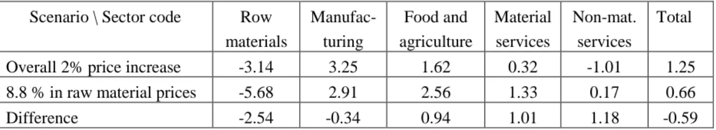
7.2. The effect of differentiating the changes in parameters across sectors ... - 32 -
8. Concluding remarks ... - 32 -
References ... - 34 -
Ernő Zalai – Tamás Révész
T
HE ISSUE OF MACROECONOMIC CLOSURE REVISITED AND EXTENDED1Abstract
Léon Walras (1874) already had realized that his neo-classical general equilibrium model could not accommodate autonomous investment. Sen analysed the same issue in a simple, one-sector macroeconomic model of a closed economy. He showed that fixing investment in the model, built strictly on neo-classical assumptions, would make the system overdetermined, thus, one should loosen some neo-classical condition of competitive equilibrium. He analysed three not neo-classical “closure options”, which could make the model well determined in the case of fixed investment. Others later extended his list and it showed that the closure dilemma arises in the more complex computable general equilibrium (CGE) models as well, as does the choice of adjustment mechanism assumed to bring about equilibrium at the macro level. By means of numerical models, it was also illustrated that the adopted closure rule can significantly affect the results of policy simulations based on a CGE model.
Despite these warnings, the issue of macro closure is often neglected in policy simulations. It is, therefore, worth revisiting the issue and demonstrating by further examples its importance, as well as pointing out that the closure problem in the CGE models extends well beyond the problem of how to incorporate autonomous investment into a CGE model. Several closure rules are discussed in this paper and their diverse outcomes are illustrated by numerical models calibrated on statistical data. First, the analyses is done in a one-sector model, similar to Sen’s, but extended into a model of an open economy. Next, the same analyses are repeated using a fully-fledged multi- sectoral CGE model, calibrated on the same statistical data. Comparing the results obtained by the two models it is shown that although, using the same closure option, they generate quite similar results in terms of the direction and – to a somewhat lesser extent – of the magnitude of change in the main macro variables, the predictions of the multi-sectoral CGE model are clearly more realistic and balanced.
1. Introduction
Beginning from the 1980s a large number of computable general equilibrium (CGE) models have been developed all over the world to study a wide range of economic policy areas and issues in which simpler, partial equilibrium or aggregate macro models would be unsatisfactory. CGE models have become standard tools in studying a variety of policy issues, including tax policies, energy and environmental policies, to evaluate the impact of EU cohesion policy and so on2.
It had been realized already by Walras (1834-1910), the father of neoclassical general equilibrium models, that in his multi-sector model, built strictly on neo-classical assumptions, there was no room for autonomous investment. Despite this early appearance of the problem, the discussion of the issue is usually traced back only to Sen (1963), who analysed this problem in a simple one-sector model, in which he showed that in the neoclassical realm investment has to be a variable, adjusting freely. He then presented three not neo-classical adjustment mechanisms, to illustrate how one could fix investment in an otherwise neo- classical model.
Sen’s analysis was later extended by Taylor and Lysy (1979) in the framework of CGE models, discussing a wider range of closure alternatives. Dewatripont and Michel (1987)
1 The research underlying this paper is made possible through the support from the European Commission (projects ÁROP 1.1.10-2011-2011-0001 and 151629-2010 A08) and personally from Juan Carlos Ciscar (EC's JRC-IPTS) as well as from the Centre for Public Affairs Studies at Corvinus University of Budapest, for which we express our gratitude.
2 From the vast literature on CGE models we refer to the books of Dervis, De Melo and Robinson (1982), Shoven and Whalley (1992), Bergman, Jorgenson and Zalai (1990), Hertel (1997).
analysed the microeconomic basis of the closure problem in the context of temporary competitive equilibrium. Some numerical investigations3 made clear that the choice of macro closure can significantly affect the policy simulation results obtained from a CGE model.
Despite these early warnings, the issue of macro closure is mostly neglected in policy simulations. It is seldom analysed how sensitive the CGE simulation results are depending on what closure option is chosen. It is, therefore, worth revisiting the issue and demonstrating its importance by further theoretical and numerical examples. It is also important to point out that the closure problem extends beyond the treatment of autonomous investment. The problem of how to close a CGE model arises in other areas as well, because, as a rule, the number of potential variables exceeds the number of equations which can be formulated on the basis of trustworthy and operational theories.
Monetary and financial forces can be treated at most in an ad hoc fashion in the CGE models, real dynamic considerations are seldom included into them either. Attempts to extend the models in these directions make them less tractable and less reliable. It can be safer to set the expected magnitude of certain economic variables exogenously rather than determining them endogenously by using formulas questionable on conceptual or empirical ground. Thus, the model builder has to fix the value of some potential macroeconomic variables, i.e., has to choose which variables will be endogenous and which exogenous (fixed) in his model.
In our paper we generalize first Sen’s model to a one-sector model of an open (rather than closed) economy, in which the single product has differentiated varieties, which are less than perfect substitutes for each other. This brings the one-sector model closer to the multisectoral CGE models. Then, based on the related literature, Sen’s analysis is extended to different, characteristic closure alternatives. The diversity of outcomes yielded by different closures is illustrated by numerical simulations based on a model calibrated using Hungarian statistical data. In the second part of the paper the same analysis is extended to a fully-fledged CGE model, including taxes/subsidies, elaborated income distribution scheme, distinguishing five production sectors and three groups of households, calibrated on the same data set.
Comparing the results of similar simulation runs, based on the same closure option and assuming the same shock, will highlight not only the qualitative similarities but also the significant quantitative differences between the results achieved by the aggregated macroeconomic and the multisectoral CGE model.
2. Prelude: the closure problem as encountered by Walras
Walras analysed the conditions of general equilibrium at different levels of abstraction in various simple models of a closed economy.4 Here we reconstruct his one-period, multi- commodity model with investment and capital goods, in which the problem of closure arose for him. His model can be seen as the reduced form of a more detailed and complex model of general equilibrium, in the framework of which the closure problem will be analysed later.
The survey of this simple and transparent model will help the reader understand better how
3 See, for example, Rattsø (1982), Taylor (1990), Decaluwe et al. (1988) and Robinson (1991, 2006), Thissen (1998).
4 See Zalai (2004) for more details on Walras’s models.
the closure problem arises and the structure of the multisectoral general equilibrium models too.
For the sake of simplicity, Walras distinguishes three types of commodities in his model:
consumer goods, natural (e.g., labour) and produced factors of production (capital goods). He left out of consideration intermediate demand for products as well as final demand for primary goods. The supply of natural factors of production and consumers’ demand for products are represented by functions of prices (homogeneous of degree zero), and fixed input coefficients are used to determine demand for the factors of production.
Unlike Walras, we do not split products into consumer and capital goods. We assume simply that any commodity could be consumed as well as accumulated as a capital good, which can be used only in the subsequent time periods, determining the capital stocks. The necessary conditions of equilibrium can be formulated as follows.
Equilibrium on the markets of products and factors of production:
xi = yic(p, q, w) + yib, i = 1, 2,…, n, (W-1)
bi1⋅x1 + bi2⋅x2 +…+ bin⋅xn = Ki, i = 1, 2,…, n, (W-2) dk1⋅x1 + dk2⋅x2 +…+ dkn⋅xn = Sk(p, q, w), k = 1, 2,…, s. (W-3) Equilibrium pricing rules (price equals cost):
pj = w1⋅d1j + w2⋅d2j +…+ ws⋅ds + q1⋅b1j + q2⋅b2j +…+ qn⋅bnj, j = 1, 2,…, n. (W-4)
qi = (ria + πi)⋅pi, i = 1, 2,…, n. (W-5)
where
• xi total (final) output of product i,
• pi the price of product i (i = 1, 2,…, n),
• qi the rental price of capital good i,
• wk the price of primary factor k (k = 1, 2,…, s),
• yic(p, q, w) consumer’s demand for product i, where p = (pi), q = (qi), w = (wk),
• yib the amount of product i invested,
• bij the input coefficients of capital goods (capital good i used per unit of product j),
• Ki the supply of capital good i (accumulated in the past),
• dkj the input coefficients of primary factors of production (primary factor k used per unit of product j),
• Sk(p, q, w) the supply of primary factors,
• ria the rate of depreciation of capital good i,
• πi the net rate of return on capital good i.
The unknowns in equations (W-1) − (W-5) are xi, yib, pi, qi, πi and wk, their number is thus 5n + s. The number of the equations is however only (4n + s), leaving n degrees of freedom for the above system of equations. Neither the rates of return (πi) nor the investment demand (yib) is yet determined according the conditions of long-run equilibrium in the above model.
The rates of return should be equalized, whereas investment should match the future demand
for capital goods. Walras became aware of the fact that he could only set one of these conditions in order to close the model. He decided to prescribe the equality of the net rates of return (π) by adding to equations (W-1) − (W-5)
πi = π, i = 1, 2,…, n, (W-6)
by which the number of the unknowns (xi, yib, pi, qi, πi, π, wk) became (5n + s + 1), and the number of the equations is (5n + s).
The same effect could be achieved by substituting
qi = (ria + π)⋅pi, i = 1, 2,…, n. (W-5a)
for equations (W-5) and dropping the variables πi. In either case the degree of freedom of the resulting model will be one, which can be eliminated by the choice of the numeraire.
Walras was aware of the fact that investment demand became residual by this choice and therefore his model represents only part of the conditions of a long-run equilibrium. He was criticized later by Keynes for his choice, who would have introduced investment demand functions based on expectations instead. By doing so, however, he would have arrived at the conditions of a temporary equilibrium rather than that of a long-run equilibrium, which Walras tried to define, but could not do it in a consistent way.
Referring to the CGE models it is interesting to note that the definition of the rental price of capital (equation W-5) introduced by Walras, is used in the applied GE models as well. It is also worth of noting, that capital goods in Walras’ model take the form of homogenous sectoral products, as in Leontief’s theoretical input-output models. In the applied multisectoral models, including the CGE models, sectoral capital goods are as a rule composite commodities, put together from homogenous sectoral products without using directly any factor of production.
3. Analysis of the closure issue in the framework of a one-sector macroeconomic general equilibrium model
Sen (1963), as mentioned, analysed the closure problem in a simple one-sector model of a likewise closed economy. We extend, first of all, Sen’s analysis to an open economy, which brings it closer to the CGE models.5 We extend Sen’s analysis also by adding to it further closure possibilities from the related literature. In addition, the results will be numerically illustrated by means of a computable model, based on statistical data.
Three basic and two composite commodity varieties of the same single product are differentiated in our model: commodity produced and sold at home, exported and imported, its composite domestic output and its composite supply on domestic market. The volume (use value) of the composites of differentiated basic products is measured by monotone increasing, linear homogenous (aggregation) functions. Unlike Sen, we take into account its intermediate use in production too.
Output capacity is defined by a nested production function of Johansen type, as common in CGE models. Labour (L) and capital (K) are assumed to be imperfect substitutes, jointly
5 Using one-sector models for didactic purposes is quite common and useful practice in the CGE literature too. See, for example, Devarajan et al. (1994) and Robinson (2006).
determining the output capacity by a linear homogeneous production function, F(L, K). In our numerical model it will be represented by a constant elasticity of substitution (CES) function.
The composite output (X) is divided between domestic (Xh) and export (Z) supply by means of a constant elasticity of transformation (CET) function, X = X(Xh, Z). Reexport, as usual, is left out of consideration as usual. The composite home supply (Xhm) of the commodity produced at home (Xh) and imported (M) is defined by a CES aggregation function, Xhm = Xhm(Xh, M).
This means that five commodity prices have to be introduced: the user’s price on the domestic (ph) and the world market (pwe), the world market price of the imported good (pwm), the producer’s price of the composite output (pa), and the users’ price of the composite domestic supply (phm). For the sake of simplicity taxes/subsidies, modifying potentially the prices, are disregarded. Therefore, the domestic equivalents of the world market export and import price are simply v⋅pwe and v⋅pwm, where v is the exchange rate.
In the case of import price we adopt the small open economy assumption, pwm will be thus an exogenous variable. In the case of export, however, as often assumed in CGE models, its world market price depends on its volume, pwe = pwe(Z). According to neo-classical theory this would mean that exports are differentiated on the world market by the area of their origin.
Each country faces thus a less than perfectly elastic export demand function, and pwe(Z) is the inverse of that demand function.
Neo-classical theory assumes that the wage rate (w) and the rental price of capital (q) has to be equal thus to the marginal revenue of labour and capital. The revenue is measured here by the value added, pa – phm⋅A, where A is the constant material input coefficient. In some of the discussed closure rules, however, factor prices will be allowed to adjust freely and depart from their marginal products, while the nonprofit pricing rule will be maintained. Therefore, the equilibrium conditions of production will be formulated in the following way:
X = F(L, K) (1), w/αw = (pa – phm⋅A)⋅
L K L F
∂
∂ ( , )
(2), pa⋅X = phm⋅A⋅X + w⋅L + q⋅K. (3) The new variable, αw in equation (2) plays the role of a switch variable. If αw is fixed at value 1, then the wage rate will be equal to the marginal revenue of labour, and by virtue of Euler’s theorem and the assumed linear homogeneity of the production function from equations (1) – (3) follows that the rental price (cost) of capital (q) is equal to its marginal revenue:
q = (pa – phm⋅A)⋅
K K L F
∂
∂ ( , )
. (3a)
In this case, equation (3) can be viewed as the equation which indirectly determines the equilibrium rental price of the capital.
If the factor prices are allowed to depart from the respective marginal products, αw
measures simply the ratio of the wage rate to the marginal revenue of labour.
For later reference it is also worth mentioning that one could also use
L = l(w/αw, q)⋅X (1’), K = k(w/αw, q)⋅X (2’)
conditions instead of (1) and (2), where l(w/αw, q) and k(w/αw, q) are the factor demand functions in the case of unit output, derived from the above conditions. In the CGE models it
is common and useful to use such dual forms. We will also use them in the specification of our CGE model.
Following Walras’s definition, the relation between the cost of capital (q) and the net rate of return on capital (π) is q = (ra + π)⋅phm. For convenience, amortization is disregarded (ra = 0), thus, this relationship reduces to q = π⋅phm.
The prices of the composite commodities are determined based on the assumption that their composition is always optimal. In the case of the domestic/export composite the total sales revenue (ph⋅Xh + v⋅pwe⋅Z) is maximized (assuming price taker individual exporters), in the case of the domestic/import composite, total costs (ph⋅Xh + v⋅pwm⋅M) is minimized. These assumed optimizations can be represented by the following first order necessary conditions:
X = X(Xh, Z) (4), ph = pa⋅ ( hh, ) X
Z X X
∂
∂ (5), v⋅pwe = pa⋅
Z Z X X
∂
∂ ( h, )
(6),
Xhm = Xhm(Xh, M) (7), ph = phm⋅ hm( hh, ) X
M X X
∂
∂ (8), v⋅pwm = phm⋅
M M X X
∂
∂ hm( h, ) (9), where the composite prices (pa and phm) are, as a matter of fact, the Lagrangian multipliers corresponding to the respective optimization problems.
Condition (6), however, has to be modified, because we assume that export demand is less than perfectly elastic. pwe defined by pwe(Z), the inverse demand function, will thus appear instead of pwe. The assumption would imply potential monopolistic position for the exporters, which could be exploited by means of so-called optimal tariffs (see, for example, Limão, 2008). In CGE models, designed for practical uses, it would not be realistic to take this theoretical possibility into consideration and price taker agents are assumed. The introduction of less than perfectly elastic export demand functions serve only the purpose to restrain price induced changes in the volume of export and vice versa.
Observe that – since the aggregation functions are by assumption linearly homogenous and by virtue of Euler’s theorem – from equations (5)-(6) and (8)-(9) one can derive:
pa⋅X = ph⋅Xh + v⋅pwe⋅Z (6a), phm⋅Xhm = ph⋅Xh + v⋅pwm⋅M. (9a) These indicate first, that the prices of the composite goods are the weighted averages of the prices of their components. Second, these derived forms could also be used as conditions of optimality, for example, instead of (6) and (9), respectively. Third, one can also derive the following conditional export supply and import demand functions from (5)-(6) and (8)-(9), respectively:
Z = reh(ph, v⋅pwe)⋅Xh (5a), M = rmh(ph, v⋅pwm)⋅Xh (8a), where reh and rmh are the optimal share coefficients, defined as functions of relative prices.
One could thus use these latter forms instead of (5) and (8). We will use such derived (dual) forms later in presenting the equations of the multi-sectoral CGE model.
Equations (1) - (9) define the equilibrium conditions for the supply of commodities for export and domestic use, the demand for imports as well as the market clearing commodity prices. They have to be completed yet with equations describing the income (re)distribution and final demand side of the model.
We will make use of many simplifying assumptions in formulating the various budget and behavioural constraints.
pwm· M − pwe(Z)·Z = De (10)
phm⋅G + Sg = τ⋅(w⋅L + q⋅K) (11)
phm⋅C + Sp = (1 – τ)⋅(w⋅L + q⋅K) (12) Sp = (1 – τ)⋅(σw⋅w⋅L + σk⋅q⋅K) (13) Equation (10) defines the trade balance deficit (De), in fact, the net savings of foreigners, since non-trade related transfers are neglected in our model. Equation (11) is the budget balance of the public household (government), where G denotes public consumption and Sg net public saving. In this model, for the sake of simplicity, government is assumed to collect revenue only from income tax6, by means of a uniform tax rate (τ) applied to both labour and capital income. Equation (12) represents the budget balance of the households, where C denotes private consumption. On the left hand side one can see the sum of the value of private consumption (phm⋅C) and net private savings (Sp), on the right one the formation of disposable (net) income. Sp is determined by equation (13), assuming different savings ratios (σw, σk) in the case of labour and capital income.
The commodity balance on the home market takes the following form:
Xhm = A⋅X + C + G + I. (14)
where I denotes investment.
By routine transformations it can be shown that equations (1)-(12) and (14) imply phm⋅(C + G + I) = w⋅L + q⋅K + v·De.
This means that final expenditure will be always equal to total income (Walras law) and investment to savings. Therefore, in most related papers, including Sen’s seminal paper itself, the reader finds equation phm⋅I = Sp + Sg + v·De instead of (14).
The real rate of exchange is defined as the ratio of the foreign to the domestic value of the produced commodity, i.e., as the domestic cost of earning one unit of foreign exchange:
vr = v·pwe(Z)/ph. (15)
The above 15 equations define the skeleton of the general equilibrium model that will be used later and we will refer to it as the basic model. The model will be well-determined if the number of variables and equations are equal. The potential (endogenous) variables exceed the number of equations, since at least the following 25 could be chosen as variable, depending on our assumptions: I, L, K, X, Xh, Xhm, Z, M, C, G, pa, ph, phm, pwm, w, wr = w/phm, αw, q, v, vr, Sp, Sg, σw, σk, τ. We will therefore refer to them as variables, to distinguish them from the parameters, which will be always constant. The actual choice of model specification will decide which of them will be endogenous and/or exogenous variable.
6 Distinguishing consumer’s price from general user’s price, income tax could be replaced by consumption tax.
4. Macro closure options in the one-sector general equilibrium model
The actual choice of model specification, i.e., the closure rule, decides which critical macro variables will remain endogenous and which become exogenous in a given model. X, Xh, Xhm, Z, M, C, pa, ph, q, v, Sp and Sg (12 altogether) will be, as usual, endogenous in each closure to be discussed below. At the same time, available capital (K), public consumption (G), world market import price (pwm) and the savings rates (σw, σk) will be fixed in all versions, although they could be endogenous variables in certain models. Either foreign saving (De) or the real rate of exchange (vr) will be fixed in each closure version too. The first case is perhaps closer to a neo-classical setup, treating foreign exchange as a scarce resource, similarly to labour and capital. As will be seen, the two cases can lead to considerably different results.
The general price level has to be set exogenously yet. It will be fixed by phm = 1, in which case w will be the nominal as well as the real wage rate (wr = w/phm), whereas, since ra = 0, the cost of capital (q) will represent at the same time the rate of return (π), because q = π⋅phm
= π (their dimensions remain though different, π refers to the value, q to the volume of capital).
Table 1: Summary of various closure rules in the one-sector model
I. neo- classical
II.
Keynesian
III.
Johansen
IV. neo- Keynesian I.
V. neo- Keynesian II.
VI. struc- turalist I.
VII. struc- turalist II.
VIII. loan- able funds
I endog. exog. exog. exog. exog. endog. endog. endog.
L exog. endog. exog. exog. endog. endog. endog. exog.
w endog. endog. endog. endog. exog. exog. endog. endog.
αw 1 1 1 endog. endog. endog. endog. 1
vr exog./
endog.
exog./
endog.
exog./
endog.
exog./
endog.
exog./
endog.
exog./
endog.
exog./
endog.
exog./
endog.
De endog./
exog.
endog./
exog.
endog./
exog.
endog./
exog.
endog./
exog.
endog./
exog.
endog./
exog.
endog./
exog.
τ exog. exog. endog. exog. exog. exog. exog. exog.
cπ na na na na na endog. exog. na
i na na na na na na na endog.
Notes: endog. = endogenous, exog. = exogenous, na = not applicable.
The basic model, discussed so far, contains 15 equations and only 12 variables have been chosen as endogenous ones so far. Three additional endogenous variables should be thus still chosen from among the remaining potential endogenous variables (I, L, w, αw, vr or De, τ) to close the model. We start the discussion of possible closure rules with the four alternatives
analysed by Sen in his simpler model of a closed economy. Table 1 provides a useful summary of various closure rules to be discussed.
I. The neo-classical (Walrasian) closure
In a neo-classical closure L would be the fixed, and the factors of production paid according to their marginal revenue.7 Thus, w is endogenous variable and αw = 1. As mentioned above, either vr or De will be also endogenous variable, whereas τ is a given parameter, influencing the disposable income of the households. Only investment (I) remains thus to be the still missing, 15th endogenous variable.
Observe that, if either De or v is exogenous variable, as assumed, as long as L is fixed and the factor prices equal their marginal revenues (αw = 1), equations (1)-(10) can be solved independently from the rest of model equations for variables X, Xh, Xhm, Z, M, w, q, ph, pa and phm (or v), which appear in them, by setting the price level as v = 1 (or phm = 1). In such a case, thus, the total supply of goods for final use is determined by the production and trade possibilities alone. The rest of the model determines only its distribution. The supply and demand side of the model depend on each other thus only if L is free to adjust and/or factor prices can depart from their marginal revenues.
The neo-classical closure rests thus on the assumption that whatever is saved will be invested, independently of the expected future demand for capital. By the same token, the capital inherited from the past (K), was formed with no concern for its present needs. This reveals clearly the roots of the closure problem.
Note also that it is not specified in this model, what sort of mechanism could make the investment adjust to savings. The interest rate is often assumed implicitly to equilibrate savings and investments, which option will appear later in the loanable funds closure.
II. Keynesian (General Theory) closure
As indicated earlier, if one wants to introduce autonomous investment into the model, he or she must relax the strict neo-classical conditions. Borrowing from Keynesian theory, Sen relaxed first the assumption of fixed labour constraint (full employment) by reinterpreting L as the variable level of employment and could thus fix the level of investment instead. Since the wage rate remains determined by the marginal revenue of labour, any increase in the level of employment will go hand in hand with its decrease and the increase of the rate of return on capital, and vice versa, establishing thus the equality between investment and savings. Any exogenous increase in investment (or government expenditure) would generate Keynesian multiplier effect in such a model.
III. Johansen closure
The third closure option discussed by Sen was inspired by Johansen’s (1960) pioneering CGE model, in which it was assumed that the government could intervene by appropriate tax policy to secure full employment even in the case of exogenously fixed investment level. In Johansen’s model, the supply of both labour and capital was fixed, and marginal pricing rule
7 It can be shown that as long as L is fixed equations (1) - (10), i.e., the production and trade possibilities determine alone the total supply of goods for final use and the rest of the model determines only its distribution.
prevailed. If one adopts these assumptions, output will be determined in the same way as in the case of the neo-classical closure. If public consumption (G) and investment is also fixed, only the level of consumption can adjust to reach equilibrium. In this closure the changing level of tax rate (τ) is assumed to bring about equilibrium. Johansen assumed that by setting tax level appropriately the government could achieve such level and generate the saving which matches the fixed investment demand. In this closure thus the tax rate (τ) becomes the adjusting variable instead of investment. Another possibility for the government to balance demand and supply would be to regulate its own spending (G) instead of the tax rate.
IV. Neo-Keynesian closures I. (forced savings)
The fourth and last option discussed by Sen was based on the “forced savings” models of Kaldor (1956) and Pasinetti (1962), which he termed as a neo-Keynesian closure. Forced savings is a macro closure scenario, in which αw becomes endogenous variable instead of the investment level. It is thus assumed that changing real wage could make savings adjust to a fixed level of investment even in the case of full employment.
Forced savings is thus a macro closure scenario, in which investment becomes exogenous variable and αw will be endogenous variable instead, but the wage rate is not equal to the marginal revenue of labour, measuring the ratio of the wage rate to the marginal revenue of labour. Compared to the Johansen closure, αw and not τ will be the new endogenous variable compensating for fixing the investment level in this case.
If the general price level is set by w = 1, instead of phm = 1, as common in Keynesian models, the output price will be the equilibrating variable, which will set the real wage and through that consumer demand to such a level that brings about equilibrium between saving and fixed investment demand. Increasing investment, for example, would drive real wage down, as in the case in the Keynesian closure. Unlike in the latter, however, the level of both employment and output remains unchanged, and increasing investment crowds out consumption.
V. Neo-Keynesian closure II. (fixed real wage)
An alternative closure also with Keynesian flavour could be one, in which real wage rate is fixed and the employment level is the equilibrating variable, as in the so-called Keynesian closure. This would combine thus two Keynesian assumptions, the refusal of the neo-classical idea of full employment as well as the marginal revenue productivity theory of wages.
VI-VII. Structuralist closures
Structuralist CGE models, designed and used mainly for analysing economic policy options in developing economies8, bring in institutional considerations in describing the behaviour of certain macroeconomic variables. Following Keynes and classical economists, they usually allow for fixed nominal or real wage rate, for unemployment (i.e., variable level of employment) and may depart in other aspects also from the neo-classical assumptions. For example, investment can depend on expected future returns, the level of capacity utilization
8 For a detailed discussion of the structuralist models see, first of all, Taylor (1990).
may vary, various market imperfections are taken into account, cost-plus-markup price formation is assumed.
We will analyse here a model, in which cost-plus-markup pricing rule is assumed and investment is a function of the net rate of return on capital (π):
I = I(π), (16)
where π can be interpreted as an index of expected future returns.
Cost-plus-markup pricing means that equation (3) is replaced by the following one:
pa⋅X = (1 + πm)⋅(phm⋅A⋅X + w⋅L), (3b)
where πm is the profit markup, which replaces the rate of return on capital.
Alternatively, one can simply introduce profit markup as a new variable, together with an additional equation that establishes the relationship between the rate of return on capital and the profit markup. Choosing this option, the following form will be used:
π⋅phm⋅K = pa⋅cπ⋅X, (17)
where cπ = πm/(1 + πm), is the ratio of profit in total revenue, replacing πm. It is worth observing that equation (17) can be rewritten as
π⋅phm⋅K = πm⋅(phm⋅A⋅X + w⋅L) =
m m
1ππ
+ pa⋅X. (17a)
These forms provide an interesting insight into the model. If profit markup (πm) is fixed, the rate of return on capital moves practically in proportion to X, which in turn changes only, if L changes into the same direction too. Thus, for example, an increase in investment will lead to an increase in the rate of return on capital, triggering an accelerator effect, in addition to the multiplier effect caused by variable employment level, although the profit markup is fixed.
After suitable rearrangement, from (17a) we get κ =
K
X = a
hm
m
1 m
p p ππ
+ π,
where κ = X/K can be interpreted as a measure capacity utilization, at least as long as the level of output is less than achievable in case of full employment (at the fixed supply of capital).
From the above equation one can see that the investment function (16) is similar to, in fact, if phm = pa (e.g., in a closed economy) it is equal to
I = I(κ, πm),
which is an investment demand function commonly used in econometric models. κ is here interpreted as an accelerator term, and πm as an index of expected future returns. As will be seen later, the investment function will indeed bring forth upwards or downwards accelerator effect in the model, in addition to the multiplier effect caused by variable employment level.
In the model extended by equations (16) and (17) five further endogenous variables remain to be chosen and their potential list is extended by variable cπ. One cannot, of course, fix both π and cπ at the same time. In the case of the two structuralist closures introduced I, L
and αw are endogenous variable, and τ remains exogenous. One has thus to choose two more from among w, πm and vr or De. We choose either vr or De, as before, thus the remaining choice is either the (real) wage rate or the profit markup. In Structuralist closure I. the wage rate, in Structuralist closure II. the profit markup will be fixed.
VIII. The loanable funds closure
Based on the classical idea that savings can be viewed as the supply of loanable funds and investment the demand for them, one could introduce into the model the real rate of interest (i) as an additional variable, and assume that the saving rates, σw(i) and σk(i) are increasing, whereas investment, I(i) a decreasing function of it. In such a model the rate of interest would be the equilibrating variable that makes investment and savings match one another. In that model the private saving identity and the investment function have to be modified as follows:
Sp = (1 – τ)⋅[σw(i)⋅w⋅L + σk(i)⋅q⋅K]. (12a)
I = I(i). (16a)
As explained by Taylor (1990), such a closure is subject to at least two serious objections (both emphasized by Keynes already). First, the interest rate, i.e., the rate of return to assets, is in principle determined by stock markets and not by saving and investment flows. Second, the influence of the interest rate on aggregate investment demand is limited by various institutional factors. It could affect only certain part of gross capital formation and purchases of durable goods. This mechanism is thus seldom used in CCE models, but Bourguignon et al.
(1991) attempted to handle this problem by incorporating cumulative flows of funds into the model.
IX. The real balances (Pigovian) closure
Continuing the above comments, the loanable funds approach can be extended into a real balances closure by taking into account wealth effects, in the form of the Pigou (1943) effect or, based on the portfolio model developed by Tobin (1971), introducing interest payments and interest clearing financial asset markets. Assuming exogenously given nominal wage and introducing money supply (M) one could define the real balances of the wealth holders (M/phm). If the saving rate depends on the real balance, the real balance effect could work in the same way as the rate of interest in the loanable funds closure.
5. A numerical example and simulation results
We selected six characteristic closure rules (I., II., III., V., VI. and VII.) to demonstrate the adjustment mechanisms assumed to work in them by means of a numerical model. We used Hungarian statistical data for 2010 to calibrate the model (Hungarian Central Statistical Office 2012, 2013). The data base used for calibration is arranged in Table 2, which can be regarded as an Input-Output (I-O) table combined with a Social Accounting Matrix (SAM) (integrating national accounts and household budget survey data). Making use of the simple structure of our models, we managed to include the income redistribution into the fourth quadrant of the table.
Table 2: The initial data arranged into a combined I-O and SAM table (values in thousand billion HUF)
Expenditures
⇒ Receipts ⇓
Commodities (composition of sources)
Consumers Government Investors Rest of the World
Total receipts
Commodities (deliveries)
phm⋅A⋅X = 31.69
phm⋅C = 10.85
phm⋅G = 6.17
phm⋅I = 4.58
v⋅pwe·Z =
20.37 73.66
Consumers w⋅L =
13.97
(1–τ)⋅(1–σk)⋅
q⋅K = 3.73 17.70
Government τ⋅w⋅L = 2.96 τ⋅q⋅K = 2.01 4.97
Investors q⋅K = 9.46 Sw = σw⋅(1–τ)⋅
w⋅L = 3.89 Sg = –1.20 v·De = –1.83 10.32 Rest of the
world
v⋅pwm·M =
18.54 18.54
Total outlays 73.66 17.70 4.97 10.32 18.54
The base level of all price indeces pa, ph, phm, pwe, pwm and that of the nominal foreign exchange rate v were set to 1 in the calibration, which with the observed L = 4 and K = 200 factor employments led to the initial values of 3.493 and 0.047 for w and q. Calibrated values of some parameters:
• πm = 0.207 ; τ = 0.212; σw = 0.353; σk = 0.5;
• the elasticity of substitution (set exogenously) and the calibrated distribution parameters (a*) in the CES-CET functions are as follows:
CES F(ϕ, aL, aK, rL, rK) = F(0.5, 0.596, 0.404, 0.0726, 3.628), where rL, and rK are the labour and capital coefficients in the base case;
CET X(σ, ad, az) = X(-2, 6.330, 53.613);
CES Xhm(µ, ah, am) = Xhm(0.5, 0.425, 0.121).
• the price elasticity, ε in the pwe(Z ) = az⋅Z-1/ε export demand function, was set at -4, which means that 1 per cent increase in export volume leads to 0.25 per cent decrease in export price. In most CGE models somewhat smaller values are used, which yield larger price effects.9
As one can see, in the case of exports we assumed that domestic and export supply can be transformed into each other with relative ease (the elasticity of transformation is 2), whereas, in the case of imports, we assumed that they are rather complements than substitutes to domestic products (the elasticity of substitution set at 0.5), which means their supply will move in the same direction.
In our simulation exercises we stick always to the rule that the external shock is created by change only in one exogenous variable. In policy simulations made with CGE models, one
9 The simulation results are rather sensitive to the size of the elasticity, especially in the case of fixed balance of trade.
designs normally a scenario, in which forecasted changes in all important exogenous variables are taken into account and harmonised with each other.
5.1. The effect of a 5% increase in the government expenditure under various closures We have chosen six closure alternatives, neo-classical (I.), Johansen (III.), Keynes (II.), neo-Keynesian II. (V.), structuralist I. and II. (VI-VII.) for illustrative exercises. We have first simulated the effect of an internal demand shock, assuming 5% increase in the government expenditure. We have estimated the results both in the case of fixed real exchange rate and fixed balance of trade. The results are shown in Table 3.
We will analyse in details only the case of fixed real exchange rate, since in the case of fixed balance of trade the real effects will be very similar, although somewhat sharpened.
Savings will behave, of course, differently in the two cases. In all but the first two simulations (closures) foreign savings decreases in the first case and – only in domestic currency - increases in the second. Private saving increases also faster (due to the larger increase of employment) and government saving increases therefore slower.
In the neo-classical and the Johansen closure total output and net output for final use, the wage and profit rate, all prices, foreign trade and foreign saving remain the same as in the base. The increase in government expenditure affects therefore only the distribution of the net output. In the case of the neo-classical closure the increase of the government expenditure takes place at the cost of investment and government saving. In the Johansen closure government expenditure increases at the expense of consumption, which is enforced by the higher tax rate, which allows at the same time to increase government saving, making up for the decreasing private saving (which is assumed to decrease proportionately with consumption).
In the Keynesian closure L becomes variable instead of I, available labour does not constrain the expansion of production. The increase in the government expenditure creates a multiplier effect: output grows by 2.6% and employment by 4.5%. The marginal product of labour, consequently the wage rate decreases by 4%, which in turn increases the rate of return on capital by almost 5%. Despite the falling wage rate, total private income and consumption increases (1.9%), multiplying the effect of the autonomous growth of final demand.
With increasing output comes increasing import (2.3%), which has to be compensated by growing export (2.6%), reinforcing also the multiplier effect. Increasing export reduces slightly the price level of export (by 0.7% leading to a terms of trade loss equivalent to 2% of total savings) and increases the nominal exchange rate (0.4%). As a result of the latter, the domestic output price diminishes too (-0.2%). Since investment is fixed, savings remain the same, but its composition changes. Government’s saving decreases by about 17%, compensated by 2.4% increase in private and 0.5% increase in foreign saving.
Table 3: The effect of 5% increase in the government expenditure (percentage changes, base values in trillion HUF or ratios)
5% increase in G 1-sector macro model
Base values
fixed real exchange rate fixed trade balance
neo-
classical Johansen Keynes neo- Keynes
structu- ralist I.
structu- ralist II.
neo-
classical Johansen Keynes neo- Keynes
structu- ralist I.
structu- ralist II.
L level of employment1 4.04 0 0 4.52 5.70 4.44 8.10 0 0 4.85 6.26 4.77 9.31
X output 55.12 0 0 2.64 3.32 2.60 4.68 0 0 2.84 3.64 2.79 5.35
Xh output for domestic use 34.75 0 0 2.64 3.32 2.60 4.68 0 0 2.82 3.62 2.77 5.32
Z export 20.37 0 0 2.64 3.32 2.60 4.68 0 0 2.86 3.67 2.81 5.40
M import 18.54 0 0 2.31 2.90 2.27 4.08 0 0 2.39 3.06 2.34 4.48
Xhm domestic supply 53.29 0 0 2.53 3.17 2.49 4.47 0 0 2.67 3.42 2.62 5.03
C private consumption 10.85 0 -2.84 1.85 3.05 2.38 3.65 0 -2.84 1.99 3.34 2.56 4.17
I investment 4.58 -6.74 0 0 0 -1.45 4.26 -6.74 0 0 0 -1.56 4.87
w real wage rate2 3.458 0 0 -4.06 0 0 -4.43 0 0 -4.36 0 0 -5.04
π (q) rate of return on capital 0.047 0 0 4.80 -1.90 -1.45 4.26 0 0 5.16 -2.10 -1.56 4.87
v nominal exchange rate 1.00 0 0 0.43 0.53 0.42 0.75 0 0 0.56 0.72 0.55 1.05
vr real exchange rate 1,00 0 0 0 0 0 0 0 0 0,15 0,19 0,15 0,29
v·pwe domestic export price 1.00 0 0 -0.23 -0.28 -0.22 -0.40 0 0 -0.15 -0.19 -0.15 -0.27
ph domestic output price 1.00 0 0 -0.23 -0.28 -0.22 -0.40 0 0 -0.30 -0.38 -0.29 -0.56
pa average price of output 1.00 0 0 -0.23 -0.28 -0.22 -0.40 0 0 -0.24 -0.31 -0.24 -0.45
Sp private saving 7.91 0 -2.84 2.44 2.06 1.62 3.77 0 -2.84 2.62 2.26 1.74 4.31
Sg government saving -1.20 25.71 -18.74 16.95 14.72 17.09 10.25 25.71 -18.74 16.26 13.61 16.43 7.96
v·De foreign saving (in HUF) -2.13 0 0 -0.50 -0.64 -0.49 -0.94 0 0 0.56 0.72 0.55 1.05
αw wage/marginal product 1.00 0 0 0 5.36 4.17 2.89 0 0 0 5.89 4.47 3.33
τ tax rate 0.20 0 11.42 0 0 0 0 0 11.42 0 0 0 0
pwe foreign export price 1.00 0 0 -0.65 -0.81 -0.64 -1.14 0 0 -0.70 -0.90 -0.69 -1.31
De foreign trade deficit -2.13 0 0 -0.92 -1.17 -0.91 -1.67 0 0 0.00 0.00 0.00 0.00
domestic savings 6.71 -4.60 0 -0.16 -0.20 -1.15 2.61 -4.60 0 0.18 0.23 -0.89 3.66
terms of trade loss/GDP 0 0 0 -0.57 -0.71 -0.56 -0.99 0 0 -0.59 -0.75 -0.58 -1.10
1 million persons 2 million HUF/year/person
In the neo-Keynesian closures the wage rate is no longer determined by the marginal product of labour (αw becomes endogenous instead of I). In its first version, discussed by Sen, L remains fixed, as in the neoclassical closure, in the second, it is let vary at the expense of fixing the real wage rate.10 We present only the results of this second, neo-Keynesian closure II, in which all other aspects are the same as in the Keynesian closure. As a result of fixed real wage rate, total wage fund grows at the same rate as the level of employment (5.7%), exceeding the growth rate of the output and the value added (pa·X – phm·A·X), which grow only by about 3%. As a result, the rate of return on capital decreases (by 2%). To make up for the lost saving the level of employment and output has to expand more than in the case of the Keynesian closure. The rest of the changes are similar to those experienced in the case of Keynesian closure.
The structuralist closures depart more drastically from the Keynesian by using markup pricing and incorporating an accelerator effect in addition to the multiplier effect, because investment depends on the rate of return on capital. We used a simple investment function of the following form:
I = I0 0 ,
δ
ππ
where we have chosen I0 and π0 to be equal to the base values of the investment and the rate of return on capital, and δ, the elasticity parameter 1. Since K is fixed, all these mean that investment will change in proportion to capital income.
In structuralist closure I. the (real) wage level is fixed, and the profit markup is free to adjust. The profit markup decreases by 4.5%, the rate of return on capital and investment both by 1.5% (δ = 1!). One can observe thus a reverse accelerator effect in this case, which slows down the growth, compared to the neo-Keynesian closure.
In structuralist closure II. the rate of the profit markup is fixed instead of the real wage.
The real wage decreases by 4.4%, the rate of return on capital as well as the investment level grows by 4.26%, adding an accelerator effect to the multiplier effect. As a result, employment increases by 8.1%, output 4.7% and consumption by 3.7%, indicating thus quite an economic boom.
In Table 3 one can also see how the simulation results are modified by fixing the balance of trade instead of the real exchange rate. This makes foreign currency scarcer, than in the previous simulations, therefore, the domestic currency devaluates, increasing the domestic value of the fixed foreign surplus, i.e., decreasing foreign saving. In the case of the neo- classical and Johansen closure, in which foreign saving remains unchanged, the results do not change either. In the case of the other closures the decreasing government and foreign saving can be made up only by growing domestic income. Therefore, the economy must grow at faster rate than in the case of fixed real exchange rate, resulting in larger terms of trade losses as well.
10 This scenario assumption is somewhat unrealistic, since real wage should decrease to some extent to enable employment to increase. But we stick to the rule to change only one assumption at one time.
5.2. The effect of a 2% increase in world market import prices under various closures In the second series of simulations we analysed the likely effect of an external shock, represented by 2% increase in the world market import prices. As can be seen in Table 4, the differences between the results obtained in the case of fixed real exchange rate and fixed balance of trade become larger. At fixed real exchange rate the trade balance deteriorates, by about 9% in all closures, which must be compensated by 1.34-1.48% devaluation, if the balance of trade is fixed. This leads to larger changes in relative prices and consequently in all volume and income variables as well.
In the case of fixed real exchange rate the increasing net foreign saving (resulting from smaller trade deficit) makes up for a large part of the lost income available for domestic use, therefore the changes in final demand are less drastic than in the case of fixed balance of trade. In the case of the neo-classical and Johansen closures the GDP (effected by terms of trade changes too) drops by about 1.6% and both the wage rate and the rate of the return on capital decreases, at roughly the same per cent.
In the Keynesian and neo-Keynesian closures the results of the neo-classical closure are almost reproduced in the case of fixed real exchange rate. This is simply due to the fact that the relative prices on the domestic and foreign markets, and consequently, the domestic and foreign supply/demand structures change only slightly. Since government expenditure and investment are fixed, the level of consumption drops as a consequence of diminishing GDP.
The case of fixed balance of trade is quite different. The growing real exchange rate increases the share of export and decreases that of import, and the resulting increase of the net export in final demand enhances the multiplier effect. The higher level of employment (3.3% and 4.7%) and consumption strengthens further the multiplier effect, especially in the case of the neo- Keynesian closure. Increasing export volume is accompanied by falling export price, which increases the terms of trade loss in both Keynesian closures.
In the case of the structuralist closures, the investment function brings in a negative accelerator effect, when the rate of return on capital drops. This happens in all cases, except for one, the case of structuralist II., with fixed trade balance. There the rate of return on capital and investment increases by close to 2%, creating quite a boom.
5.3. The effect of the less than perfectly elastic export demand
The assumption of less than perfectly elastic export demand function, which is quite common in CGE models, deserves a brief comment at the end. We used the following form:
pwe(Z ) = az⋅Z-1/ε
where ε is the price elasticity of export demand, and az a constant shift parameter, which represents the export price level of the competing countries.
The price elasticity of demand was set at a reasonable large value of 4 (i.e. -4) in our scenarios, which means that 1 per cent increase in export volume will be accompanied by 0.25 per cent decrease in export price. In most CGE models somewhat smaller values are used, which yield larger price effects. (Sometimes one can even see elasticity smaller than 1, which means that a reduction in export volume will increase export revenue!!)