Mőhelytanulmányok Vállalatgazdaságtan Intézet
1093 Budapest, Fıvám tér 8.
(+36 1) 482-5566, Fax: 482-5567
www.uni-corvinus.hu/vallgazd
Analysis of purchasing activity with discounted cash flow inventory models
Imre Dobos Gyöngyi Vörösmarty
132. sz. M ő helytanulmány HU ISSN 1786-3031
2010. augusztus
Analysis of purchasing activity with discounted cash flow inventory models
Imre Dobos Gyöngyi Vörösmarty
Department of Logistics and Supply Chain Management Institute of Business Economics
Corvinus University of Budapest
Budapesti Corvinus Egyetem, 1093 Budapest, Fıvám tér 8.
Beszerzési tevékenység elemzése diszkontált pénzáramlású készletmodellel
Absztrakt.
A klasszikus tételnagyság probléma két fontosabb készletezési költséget ragad meg: rendelési és készlettartási költségek. Ebben a dolgozatban a vállalatok készpénz áramlásának a beszerzési tevékenységre gyakorolt hatását vizsgáljuk. Ebben az elemzésben a készpénzáramlási egyenlıséget használjuk, amely nagyban emlékeztet a készletegyenletekre.
Eljárásunkban a beszerzési és rendelési folyamatot diszkontálva vizsgáljuk. A költségfüggvény lineáris készpénztartási, a pénzkiadás haszonlehetıség és lineáris kamatköltségbıl áll. Bemutatjuk a vizsgált modell optimális megoldását. Az optimális megoldást egy számpéldával illusztráljuk.
Kulcsszavak: Nettó jelenérték, Diszkontált cash flow, Készpénzáramlási probléma, Készletezési modell, Beszerzés
Abstract.
The classical economic order quantity model has two types of costs: ordering and inventory holding costs. In this paper we try to investigate the effect of purchasing activity on cash flow of a firm. In the examinations we use a cash flow identity similar to that of in inventory modeling. In our approach we analyze the purchasing and ordering process with discounted costs. The cost function of the model consists of linear cash holding, linear opportunity cost of spending cash, and linear interest costs. We show the optimal solution of the proposed model.
The optimal solutions will be presented by numerical examples.
Keywords: Net present value, discounted cash flow, cash balance problem, inventory models, purchasing
1. Introduction
The cash balance model was first analyzed by Baumol (1952). He has applied the classical EOQ inventory model to investigate the demand of a firm for cash. This model is a deterministic cash model. Other deterministic cash balance problems was examined by Mensching, Garstka and Morton (1978). They have analyzed a simple cash balance problem similar that of aggregate production planning problems The analysis is seeking of an optimal solution and the planning horizons. Chand and Morton (1982) have supplied a further examination of the deterministic cash balance problem in direction of the planning horizons.
Sethi and Thompson (1970) have modeled a two-asset dynamic cash balance problem. They have solved the problem with the help of Pontryagin’s maximum principle. The solution is a bang-bang optimal control. An introductory cash management chapter is presented in textbook of Ross and Westerfield (1988)
The first stochastic cash balance model was initiated by Miller and Orr (1966). This basic model was generalized in several direction, e.g. Eppen and Fama (1968, 1969, 1971), Girgis (1968), Neave (1970), Porteus (1972), Heyman (1973), Kamin (1975), Constantinides (1976), Inderfurth and Schneeweiss (1978), Constantinides and Richard (1978). These stochastic models are solved with dynamic programming and under different cost structure. The mentioned models are critically examined by Daellenbach and asked, whether these models fit the practice.
Other papers investigate the cash management practices in the context of cash flow, e.g.
Gitman, Moses and White (1979), Morris (1983), Sartoris and Hill (1983) Vickson (1985), and Premachandra (2004). A good introduction in the stochastic cash management problems are supplied by Tapiero (1990), who presents the basic models with solution propositions.
Thorstenson (1988) has examined the capital costs in the inventory models. In his work Thorstenson has investigated the effect of discounting in cash flow inventory models. Our approach is similar that of Thorstenson. The aim of the paper is to analyze the allocation of cash in purchasing activity. The proposed model is a dynamic cash flow model with discounted costs. The cash flow identity consists of cash transfer, credit and cash requirements. The goal function has three linear elements cash holding, cash transfer, and interest costs. We solve this problem with linear programming.
The second part of the paper shows parameters, variables and goal function of the model. The next chapter characterizes some properties of the optimal solution. The fourth part presents some numerical examples, and last we summarize the results of the paper.
- xit required quantity of the ith product or service in the tth period, - Xt the cash requirements in the tth period,
- h the holding cost of cash,
- c opportunity cost of spending cash to buy products and services, - i interest rate of credit.
The variables of the model:
- It available cash level in time t, nonnegative,
- Yt cash transfer paid for products and services in period t, nonnegative, - Ct credit requirements in period t, nonnegative.
Let us assume that cash requirements of the firm are given for the purchasing department. If the prices (pit) and the required quantities (xit) of products and services are known in any period, then these requirements can be calculated as follows:
∑
=
⋅
= n
i
t i t i
t p x
X
1
,
where number n is the number of the sum of products and services.
In this model we assume that the cash flow of the purchasing department can be modeled as an inventory balance equation. The inventory balance equation consists of the sum of spent cash by purchasing department (Yt) and used credit (Ct) reduced by the cash requirements (Xt) defined above:
t t t t
t I Y C X
I = −1+ + − (t=1,2,… T), (1)
I0 is given and equal to zero.
Let us assume that the purchasing department disposes of a given quantity of money:
M Y
T
t
t ≤
∑
=1
. (2)
We assume that the variables of the model are nonnegative:
It≥ 0, Yt≥ 0, Ct≥ 0 (t=1,2,… T). (3)
The goal function of the model is the sum of the discounted period costs:
( )
min) 1 (
1
1
1 ⋅ ⋅ + ⋅ + ⋅ →
∑
+= −
T
t
t t
t h It c Y i C
r . (4)
We will analyze the optimal solution of model (1)-(4).
3. Properties of the optimal solution of the model (1)-(4)
Model (1)-(4) is a linear programming problem. Before we solve this problem we give some properties of the model. We investigate the dependence of the model on the parameters. First we examine the dependence of optimal solution on the cost parameters c and i. Then we analyze the solution in dependence on available cash (M) and the sum of the required cash
∑
= T
t
Xt 1
for purchasing.
Let us assume that the optimal solution of model (1)-(4) is
{
Ito,Yto,Cto}
T1 .The next property shows that the optimal inventory level is zero along the planning horizon.Property 1.
In the optimal solution the cash levels are zero in the planning horizon:
(
t T)
Ito =0, =1,2,..., . Proof.
(a) It is assumed that c > i. Let us reformulate the goal function a follows:
( ) ∑ [ ( ) ( ) ]
∑
= −
= − ⋅ ⋅ + ⋅ + + − ⋅
= +
⋅ +
⋅ +
⋅ + ⋅
T
t
t t
t t t
T
t
t t
t t h I i Y C c i Y
C r i Y c I
r h 1
1 1
1 (1 )
1 )
1 (
1 .
In this formula using (1) we can write
t t t t
t C I I X
Y + = − −1+ . (5)
Substituting (5) in the reformulated goal function we have
( ) ( )
[ ]
) . 1 ( )
1 ( )
1 ( 1
) 1 (
1 ) 1 (
1
0 1
1 1
1 1
1
1
1 1
1
I r i
i X r Y
i I c
r i I h
r i h r r
Y i c C Y i I r h
T
t
t t t
T
t T t T T
t
t t T
t
t t
t t t
⋅ + −
⋅ + + ⋅
+ − + ⋅
+ +
⋅
⋅
+ + + ⋅
=
⋅
− + +
⋅ +
⋅ + ⋅
∑
∑
∑
∑
= −
= −
−
−
= −
= −
The goal function has a lower bound: 0
1
) 1
1
( i I
r i X
T
t
t
t − ⋅
⋅
∑
+= − , because the cash levels and cash transfers are not lower then zero. This lower bound is achieved if values I and to Y to
In this formula substituting (5) the goal function can be written in the following way:
( ) ( )
[ ]
) . 1 ( )
1 ( )
1 ( 1
) 1 (
1 ) 1 (
1
0 1
1 1
1 1
1
1
1 1
1
I r c
c X r C
c I i
r c I h
r c h r r
C c i C Y c I r h
T
t
t t t
T
t T t T T
t
t t T
t
t t
t t t
⋅ + −
⋅ + + ⋅
+ − + ⋅
+ +
⋅
⋅
+ + + ⋅
=
⋅
− + +
⋅ +
⋅ + ⋅
∑
∑
∑
∑
= −
= −
−
−
= −
= −
The lower bound of this cost function is 0
1
) 1
1
( c I
r c X
T
t
t
t − ⋅
⋅
∑
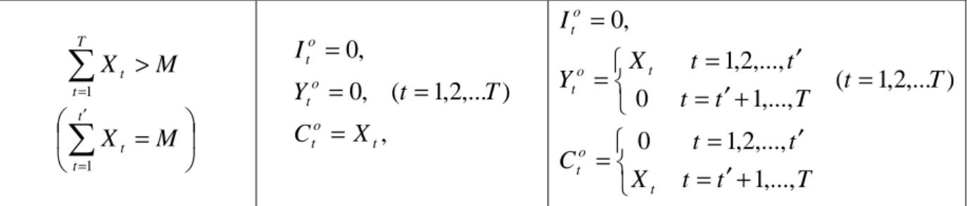
+= − . This lower bound is achieved if Ito =0,Yto = Xt,Cto =0 (t =1,2,...T), i.e. we have attained the optimal solution. This optimal solution holds if X M
T
t
t ≤
∑
=1. If X M
T
t
t >
∑
=1, then the optimal solution has the next form: Ito =0, (t =1,2,...T) and
′+
=
= ′
= t t T
t t
Yto Xt
,..., 1 0
,..., 2 ,
1 ,
′+
=
= ′
= X t t T
t C t
t o
t 1,...,
,..., 2 , 1
0 .
Time period t’ is defined as X M
t
t
t =
∑
′=1
. With these calculations we have proven the property.
Using the proof of Property 1., we have two additional properties.
Property 2.
If c > i, then in the optimal solution Yto =0,Cto = Xt, (t=1,2,...T).
The meaning of this property is that if the unit cost of cash transfer is greater than the interest rate, then it is better to use bank loan, and not to spend the asset of the firm.
Table 1. Optimal solution of the model in dependence of parameters
c > i i ≥ c
M X
T
t
t ≤
∑
=1
,
) ,...
2 , 1 ( , 0
, 0
t o t o t o t
X C
T t
Y I
=
=
=
=
, 0
) ,...
2 , 1 ( , , 0
=
=
=
=
o t
t o t
o t
C
T t
X Y I
M X
T
t
t >
∑
=1
∑
′ ==
M X
t
t t 1
,
) ,...
2 , 1 ( , 0
, 0
t o t o t o t
X C
T t
Y I
=
=
=
=
′+
=
= ′
=
=
′+
=
= ′
=
=
T t
t X
t C t
T T t
t t
t t
Y X I
t o t o t t
o t
,..., 1 ,..., 2 , 1 0
) ,...
2 , 1 ,..., (
1 0
,..., 2 , 1 ,
0
Property 3.
If i ≥ c, then in the optimal solution
(a) if X M
T
t
t ≤
∑
=1,Ito =0,Yto = Xt,Cto =0 (t =1,2,...T), and
(b) if X M
T
t
t >
∑
=1
,
′+
=
= ′
= t t T
t t
Yto Xt
,..., 1 0
,..., 2 ,
1 and
′+
=
= ′
= X t t T
t C t
t o
t 1,...,
,..., 2 , 1
0 , where
M X
t
t
t =
∑
′=1
and t’ < T.
This third property shows that it is more rational to spend the asset of the firm if the interest rate is not smaller than the opportunity cost of spending cash. The results can be summarized in Table 1.
4. Numerical examples
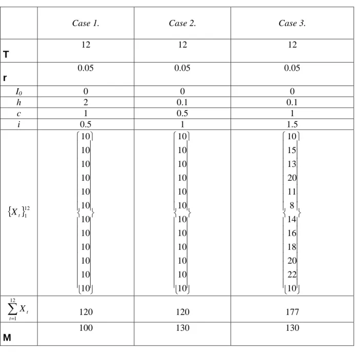
Table 1 presents three different cases of the optimal solutions. We construct problems to demonstrate the solutions with the help of data from the Table 2.
Case 1.
In this case the opportunity cost of cash transfer (c = 2) is greater than the interest rate (i
=0.5). The solution for this type of models is borrowing from a bank and using the asset of the firm for other investments. The optimal solution then Ito =0,Yto =0,Cto =10, (t = 1,2,…,12).
The minimal costs are $ 46.532.
Case 2.
The opportunity costs (c = 0.5) are lower than then interest rate (i = 1). In this model it is
∑
12 =Table 2. Parameters of the models
Case 1. Case 2. Case 3.
T
12 12 12
r
0.05 0.05 0.05
I0 0 0 0
h 2 0.1 0.1
c 1 0.5 1
i 0.5 1 1.5
{ }
Xt 121
10 10 10 10 10 10 10 10 10 10 10 10
10 10 10 10 10 10 10 10 10 10 10 10
10 22 20 18 16 14 8 11 20 13 15 10
∑
= 12
1 t
X t 120 120 177
M
100 130 130
Case 3.
The opportunity costs (c = 1) are lower than then interest rate (i = 1.5). In this model it is better to spend the available cash for purchasing, as it was in case 2. The sum of the required
cash
∑
==
177
12
1 t
Xt is lower than the available asset (M = 130). It means that the purchasing department must borrow some money from a bank. The sum of the borrowed cash is equal to
$ 43 = X M
t
t −
∑
= 12
1
. It is known in this model that 125 130
10
1
=
<
=
∑
=
M X
t
t , i.e. in the 10th period there are use of asset and borrowing. The optimal solution then Ito =0 (t = 1,2,…,12),
{
10,15,13,20,11,8,14,16,18,5,0,0}
=
o
Yt , and Cto =
{
0,0,0,0,0,0,0,0,0,15,22,10}
. The minimal costs are $ 149.429.5. Conclusions
In this paper we have investigated a discounted cash flow purchasing model. In the optimal solution of the model the cash levels are equal to zero in the planning horizon. The cash transfer is equal to zero in the model if the opportunity costs of transfer are higher than that of interest rate. If the interest rate is higher than the transfer costs, then it is optimal to spend all available cash, and if it is necessary to borrow some money from a bank.
This basic model can be generalized in several ways. A possible generalization is to take into account the date of payment. In this model form we have not examined the net present value representation of the cash flow identity. Introduction of this term can be near to the real word practice.
References
1. Baumol, W.J. (1952): The transactions demand for cash: An inventory theoretic approach, Quarterly Journal of Economics 66, 545-556
2. Chand, S., Morton, T.E. (1982): A perfect planning horizon procedure foa a cash balance problem, Management Science 28, 652-669
3. Constantinides, G.M. (1976): Stochastic cash management with fixed and proportional transactions costs, Manegement Science 22, 1320-1331
4. Constantinides, G.M., Richard, S.F. (1978): Existence of optimal simple policies for discounted-cost inventory and cash management in continuous time, Operations Research 26, 620-636
5. Daellenbach, H.G. (1974): Are cash management optimization models worthwile?, Journal of Financial and Quantitative Analysis 9, 607-626
6. Eppen, G.D., Fama, E.F. (1968): Solutions for cash-balance and simple dynamic- portfolio problems, The Journal of Business 41, 94-112
7. Eppen, G.D., Fama, E.F. (1969): Cash balance and simple dynamicmportfolio problems with proportional costs, International Economic Review 10, 119-133
8. Eppen, G.D., Fama, E.F. (1971): Three asset cash balance and dynamic portfolio problems, Management Science 17, 311-319
9. Girgis, N.M. (1968): Optimal cash balance levels, Manegement Science 15, 130-140 10. Gitman, L.J., Moses, E.A., White I.T. (1979): An assessemt of corporate cash
management practices, Financial Management/Spring, 32-41
11. Haley, C. W., Higgins, R.C. (1973): Inventory policy and trade credit financing, Management Science 20, 464-471
16. Miller, M.H., Orr, D. (1966): A model of the demand for money by firms, Quarterly Journal of Economics 80, 413-435
17. Morris, J.R. (1983): The role of cash balances in firm valuation, Journal of Financial and Quantitative Analysis 18, 533-545
18. Neave, E.H. (1970): The stochastic cash balance problem with fixed costs for increases and decreases, Management Science 16, 472-490
19. Porteus, E.L. (1972): Equivalent formulations of the stochastic cash balance problem, Management Science 19, 250-253
20. Premachandra, I.M. (2004): A diffusion approximation model for managing cash in firms: An alternative approach to the Miller-Orr model, European Journal of Operational Research 157, 218-226
21. Robichek, A.A., Teichroew, D., Jones, J.M. (1965): Optimal short term financing decision, Management Science 12, 1-36
22. Ross, S.A., Westerfield, R.W. (1988): Corporate finance, Times Mirror/Mosby College Publ., St. Louis et al.
23. Sartoris, W.L., Hill, N.C. (1983): A generalized cash flow approach to short-term financial decisions, The Journal of Finance 38, 349-360
24. Sethi, S.P., Thompson, G.L. (1970): Applications of mathematical control theory to finance: Modeling simple dynamic cash balance problems, Journal of Quantitative and Financial Analysis 5, 381-394
25. Tapiero, C.S. (1990): Applied stochastic models and control in management, North- Holland, Amsterdam et al.
26. Thorstenson, A. (1988): Capital costs in inventory models – A discounted cash flow approach, Production-Economic Research in Linköping, PROFIL 8, Linköping
27. Vickson, R.G. (1985): Simple optimal policy for cash management: The average balance requirement case, Journal of Financial and Quantitative Analysis 20, 353-369