Characterization of coronary atherosclerosis on computed tomography using advanced image processing techniques

(1)

Characterization of coronary atherosclerosis on computed tomography using advanced image

processing techniques

PhD Thesis

Márton József Kolossváry MD

Doctoral School of Basic and Translational Medicine Semmelweis University

Supervisor: Pál Maurovich-Horvat MD, PhD Official reviewers: Pál Kaposi Novak MD, PhD

Gál Viktor MD, PhD Head of the Complex Examination Committee:

Tivadar Tulassay MD, PhD

(2)

2.4. Defining the potential effect of image reconstruction algorithms on reproducibility of volumetric and radiomic signatures of coronary lesions on coronary CTA ... 34 2.5. Defining the potential of using radiomic markers as inputs to machine learning models to identify advanced atherosclerotic lesions as assessed by histology ... 34 3. METHODS ... 35

3.1. Study design and statistics for defining the effect of using coronary CTA to assess coronary plaque burden as opposed to ICA... 35 3.2. Study design and statistics for defining the potential of using radiomics to identify napkin-ring sign plaques on coronary CTA ... 37 3.3. Study design and statistics for defining the potential of radiomics to identify invasive and radionuclide imaging markers of vulnerable plaques on coronary CTA 40

3.4. Study design and statistics for defining the potential effect of image reconstruction algorithms on reproducibility of volumetric and radiomic signatures of coronary lesions on coronary CTA ... 43 3.5. Study design and statistics for defining the potential of using radiomic markers as inputs to machine learning models to identify advanced atherosclerotic lesions as assessed by histology ... 46 4. RESULTS ... 50

4.1. Comparison of quantity of coronary atherosclerotic plaques detected by coronary CTA versus ICA ... 50

(4)

4.5. Identification of advanced atherosclerotic images using radiomics-based

machine learning validated using histology ... 74

5. DISCUSSION ... 80

5.1. Coronary CTA for the characterization of plaque burden ... 80

5.2. Potential of radiomics to identify napkin-ring sign plaques ... 82

5.3. Possibility to identify radionuclide and invasive imaging markers using non- invasive coronary CTA ... 85

5.4. Robustness of volumetric and radiomic features to image reconstruction algorithms ... 89

5.5. Potential of radiomics-based machine learning to classify coronary lesions to corresponding histology categories ... 91

6. CONCLUSIONS... 93

7. SUMMARY ... 96

8. ÖSSZEFOGLALÁS ... 97

9. BIBLIOGRAPHY ... 98

10. CANDIDATE'S PUBLICATIONS ... 124

10.1. Publications discussed in the present thesis ... 124

10.2. Publications not related to the present thesis ... 124

11. ACKNOWLEDGEMENTS ... 130

(5)

ABBREVIATIONS

ACS acute coronary syndrome AI artificial intelligence AUC area under the curve CAD coronary artery disease

CI confidence interval

CNR contrast-to-noise ratio

CT computed tomography

CTA computed tomography angiography CVD cardiovascular diseases

D dimension

DL deep learning

FBP filtered back projection FFR fractional flow reserve

GLCM gray-level co-occurrence matrix GLRLM gray level run length matrix

GTSDM gray-tone spatial dependencies matrix

HU Hounsfield unit

HIR hybrid iterative reconstruction ICA invasive coronary angiography ICC intra-class correlation coefficient IQR interquartile range

IVUS intravascular ultrasound LDL low-density lipoproteins

MACE major adverse cardiovascular events MIR model-based iterative reconstruction

(6)

ROC receiver operating characteristics ROI region of interest

SD standard deviation

SIS segment involvement score SISi segment involvement score index SNR signal-to-noise ratio

SSS segment stenosis score

SSSi segment involvement score index TCFA thin-cap fibroatheroma

(7)

1. INTRODUCTION

Despite advancements in the diagnosis and therapy of cardiovascular diseases (CVD), it still remains the leading cause of morbidity and mortality worldwide (1, 2). Numerous anthropometric and lab-based risk models have been established to predict CVD (3-6).

Multiethnic evaluation of these models showed systematic overestimation of CVD risk by up to 115%, indicating the need for more precise risk estimation (7, 8). Coronary artery disease (CAD), the leading pathology behind CVD is a progressive disease of the intimal layer of the coronaries, which can cause acute and/or chronic luminal obstruction (9).

Computed tomography (CT) based technologies have evolved considerably in recent years (10). Coronary CT angiography (CTA) has emerged as a useful and highly reliable imaging modality for the examination of the coronaries and is considered as a non- invasive alternative to invasive coronary angiography (ICA) (11). With its excellent sensitivity and negative predictive value, coronary CTA is a robust diagnostic test to rule out severe coronary stenosis and it is widely used as a “gate-keeper” for ICA (12-15).

Even though, numerous studies have validated the diagnostic performance of CTA for the detection of obstructive coronary artery disease, as compared to ICA as reference standard, only a few studies have compared these two modalities regarding semi- quantitative plaque burden measurements (16, 17).

Modern CT scanners allow not only the visualization of the coronary lumen as ICA, but also the vessel wall granting non-invasive analysis of atherosclerosis itself (18). With around half of plaque ruptures occurring at lesion sites with smaller than 50% diameter stenosis, plaque morphology assessment seems equally as important as stenosis assessment (19-21). Four distinct plaque characteristics have been linked to major adverse cardiovascular events (MACE) using coronary CTA (18). Out of these four characteristics positive remodeling, low-attenuation and spotty calcification are

(8)

Radiology images are multi-dimensional (D) datasets, where each voxel value represents a specific measurement based on some physical characteristic (24). Radiomics is the process of obtaining quantitative parameters from these spatial datasets, in order to create

‘big data’ datasets, where each lesion is characterized by hundreds of different parameters (25). These features aim to quantify morphological characteristics difficult or impossible to comprehend by visual assessment (26). Radiomics has proven to be a valuable tool in oncology (27). Several studies have shown radiomics to improve the diagnostic accuracy (28, 29), staging and grading of cancer (30), response assessment to treatment (31-33) and also to predict clinical outcomes (34, 35). However, application of radiomics in cardiovascular imaging is lacking.

The vast information present in radiological images not only allows to objectively identify pathologies as opposed to current irreproducible visual classification schemes, but also to expand the capabilities of an imaging technique. Implementing radiomics with machine learning (ML) and artificial intelligence (AI) may allow to increase the abilities of coronary CTA imaging to allow better identification of vulnerable plaques by localizing plaques with metabolic activity, or by identifying the exact histological category of a given lesion using simple CT images.

The current thesis aims to assess the potentials of advanced image analysis of atherosclerosis using coronary CTA images.

(9)

1.1. Imaging atherosclerosis using CTA in clinical practice

Atherosclerosis is initiated by deposition of low-density lipoproteins (LDL) in the intima.

With oxidation of the lipids, an inflammatory response is triggered, which is characterized by macrophages engulfing oxidized LDL particles, thus becoming foam cells (36). Poorly understood genetic and environmental factors propagate inflammation, resulting in further deposition of lipids, deterioration of the extracellular matrix and cell death (37).

These processes lead to distinct plaque morphologies, which have been identified on histological samples (38).

After the first description of CTA in 1992 (39, 40), further technological advances, such as: more powerful X-ray tubes, faster gantry rotation times, multiple parallel detector rings and decreased slice thickness (41, 42) were introduced which allowed the visualization of the coronary arteries (43). With its excellent sensitivity and negative predictive value (12, 14), coronary CTA is a robust diagnostic test to rule out severe coronary stenosis and it is widely used as a “gate-keeper” for ICA (13, 15). Coronary CTA is currently the first imaging choice for stable chest pain patients in the United Kingdom and is a class 1 recommendation for initial testing of CAD based-on the European Society of Cardiology (44).

Nevertheless, modern CT scanners allow not only the visualization of the coronary lumen as ICA, but also the vessel wall, granting non-invasive analysis of atherosclerosis. This unique property of coronary CTA holds many advantages for patient risk stratification that other non-invasive tests do not. With submillimeter resolution coronary CTA allows non-invasive morphological assessment of coronary atherosclerosis.

Coronary CTA is interpreted based-on the guidelines of the Society of Cardiovascular Computed Tomography (45). Coronary plaques can be classified as being non-calcified, partially calcified or calcified based on the amount of calcium in the lesion. Furthermore,

(10)

1.2. Assessment of plaque composition using coronary CTA

1.2.1. Degree of calcification

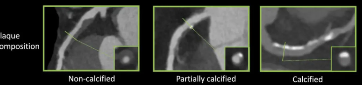
Coronary plaques can be classified as being non-calcified, partially calcified or calcified based on the amount of calcium in the lesion (figure 1).

Figure 1. Representative images of plaque characteristics identifiable using coronary CTA (46).

Coronary plaques can be classified as non-calcified, partially calcified and calcified based-on the degree of calcification present in the plaque. Curved multiplanar images are shown with a corresponding cross-section at the site of the solid line.

Large multicenter cohorts such as the COronary CT Angiography EvaluatioN For Clinical Outcomes: An InteRnational Multicenter registry (CONFIRM) (47), investigated the prognostic value of plaque composition on all-cause mortality. Based on 17,793 suspected CAD patients’ 2-year survival data, the number of segments with partially calcified or calcified plaque had a significant effect on mortality (hazard ratios: non- calcified: 1.00, p = 0.90; partially calcified: 1.06, p ≤ 0.0001; calcified: 1.08, p ≤ 0.0001).

After adjusting for clinical factors, none of the plaque components improved the diagnostic accuracy of the model (non-calcified: p = 0.99; partially calcified: p = 0.60;

calcified: p = 0.10) (48). Hadamitzky et al. found similar results when investigating the prognostic effect of plaque composition on 5-year mortality rate based on suspected CAD patients. After adjusting of clinical risk based on the Morise score (49), only the number of segments with calcified plaques improved significantly the diagnostic accuracy of the model (non-calcified: p = 0.083; partially calcified: p = 0.053, calcified: p =0.041) (50).

Dedic et al. found similar results in a different patient population. When investigating the effects of different plaque components of non-culprit lesions on future MACE in acute coronary syndrome (ACS) patients, they found none of the plaque types to have a significant impact on future MACE rates (hazard ratios: non-calcified: 1.09, p = 0.11;

(11)

partially calcified: 1.11, p = 0.35; calcified: 1.11, p = 0.15) (51). Interestingly Nance et al. found very different results when analyzing 458 patients’ data, who presented to the emergency room with acute chest pain but based on ECG and serum creatinine had inconclusive results and thus underwent coronary CTA. All patients had low to intermediate risk for CAD. After a follow-up of 13 months, they split the patients into three groups: only non-calcified plaques; exclusively calcified plaques; any partially calcified plaque or both non-calcified and calcified plaques. After adjustment for clinical characteristics and calcium-score they found the following hazard ratios: 57.64 for non- calcified, 55.76 for partially calcified and 26.45 for patients with solely calcified plaques (52). The difference compared to other studies might be due to the different methodological approach used. While previously mentioned papers examined the effect of plaque composition on a segment based level incrementally, giving the hazard ratio of an increase in the number of segments with a given plaque type, Nance et al. reported the results on a patient based level dichotomized, giving the hazard ratio of having a specific type of plaque as compared to patients without any plaques.

Overall, the effect of plaque composition on mortality still remains controversial. It seems simply classifying plaques based on the amount of calcium present holds little information regarding clinical outcome. These findings suggest, that identification of more complex morphologies is needed for better prediction of adverse outcomes.

1.2.2. Plaque attenuation pattern

Histopathologic examinations demonstrated that thin-cap fibroatheromas (TCFA) exhibit similar plaque morphologies as ruptured plaques (38, 53). TCFAs are composed of a lipid-rich necrotic core surrounded by a thin fibrotic cap. Coronary CTA is capable of distinguishing between lipid-rich and fibrotic tissue based on different CT attenuation values, however the reliable classification of non-calcified plaques into these two

(12)

into ones with NRS and ones without (22). NRS plaques are characterized by a low attenuation central area, which is apparently in touch with the lumen, encompassed by a higher attenuation ring-like peripheral area (18).

Figure 2. Representative images of plaque attenuation patterns (46).

Non-calcified plaque regions may be classified as homogeneous, heterogeneous and the napkin-ring sign, which is one of the four high-risk plaque features. Curved multiplanar images are shown with a corresponding cross-section at the site of the solid line.

The napkin-ring sign has been identified as a specific imaging biomarker of vulnerable plaques. So called high-risk plaque features aim to identify plaque prone to rupture.

Overall, four high risk plaque features have been identified to date: the napkin-ring sign, low attenuation, spotty calcification and positive remodeling.

(13)

1.3. Assessment of high-risk plaque features using coronary CTA

High-risk plaque features have been identified in the literature to indicate morphologies which might be prone of plaque rupture (figure 2-3). These are the NRS, low attenuation, spotty calcification and positive remodeling.

Figure 3. Representative images of high-risk plaque features (46).

Next to the napkin-ring sign plaque (figure 2), three further plaque imaging markers have been linked to major adverse cardiac events. Curved multiplanar images are shown with a corresponding cross-section at the site of the solid line.

HU: Hounsfield unit

1.3.1. Napkin-ring sign

Maurovich-Horvat et al. showed based on ex-vivo examinations that NRS plaques have excellent specificity and low sensitivity (98.9%; 24.4%, respectively) to identify plaques with a large necrotic core, which is a key feature of rupture prone TCFA’s (54).

Histological evaluation of NRS plaques showed that NRS plaques had greater area of lipid-rich necrotic core (median 1.1 vs. 0.5 mm², p = 0.05), larger non-core plaque area (median 10.2 vs. 6.4 mm², p < 0.01) and larger vessel area (median 17.1 vs. 13.0 mm², p

< 0.01) ascompared to non-NRS plaques (55). Interestingly, these results are in line with Virmani et al. who investigated the morphology of ruptured plaques (38). Furthermore, results of the Rule Out Myocardial Infarction/Ischemia Using Computer-Assisted

(14)

as compared to stable angina patients (culprit: 49.0% vs. 11.2%, p < 0.01, respectively;

non-culprit: 12.7% vs. 2.8%, p < 0.01, respectively) (56). Otsuka et al. conducted the first prospective clinical trial to assess the predictive values of NRS plaques for future ACS events (57). They showed that NRS plaques were significant independent predictors of later ACS events (hazard ratio: 5.55, CI: 2.10–14.70, p < 0.001). Similarly, Feuchtner et al. showed NRS to have the highest hazard ratio (7.0, CI: 2.0 - 13.6) over other high risk features when investigating 1469 patients with a mean follow-up of 7.8 years (58).

Overall it seems the napkin-ring sign has additive information beyond simple plaque composition information. However, with many factors effecting assessment of attenuation patterns, we only have limited censored information regarding the prognostic effect of these entities.

1.3.2. Low attenuation

Several studies have investigated the use of region of interest (ROI) to define the plaque components using coronary CTA as compared to intravascular ultrasound (IVUS) as the gold standard of in vivo plaque characterization (59-62). These validation studies were able to find significant differences in mean Hounsfield unit (HU) values for the different plaque components, however there is a considerable overlap between these categories (121 ± 34 HU vs. 58 ± 43 HU, p < 0.001) (60). Several studies were inspired by these results and found lower mean and minimal attenuation values of plaques in ACS patients as compared to plaques of stable angina patients (63-65). However, there was still a significant overlap in attenuation values between the two groups. Nevertheless, Motoyama et al. showed that with the use of a strict cut-off value (<30 HU), ACS patients have significantly more low attenuation plaques as compared to stable angina patients (79% vs. 9%, p < 0.001), suggesting low attenuation to be a useful marker for identifying vulnerable patients (66). Marwan et al. proposed a more quantifiable approach using quantitative histogram analysis. For all cross-sections for each plaque, a histogram was created from the CT attenuation numbers, and the percentage of pixels with a density ≤30 HU was calculated. They found similarly overlapping HU values for lipid-rich versus fibrous plaques. However, using a cut-off value of 5.5% for pixels with ≤30 HU, they were able to differentiate between predominantly lipid-rich plaques versus predominantly fibrous plaques (sensitivity: 95%; specificity: 80%; area under the curve: 0.9) using IVUS

(15)

as reference standard (67). Despite these encouraging results, there is still a major concern because of the overlapping HU values of different plaque components. Furthermore, several studies have shown slice thickness (68), imaging protocols (69), tube voltage settings (70), intra coronary contrast attenuation values (71), reconstruction algorithms, filters and noise (68, 72) all to influence CT attenuation values.

Overall, it seems discrimination of non-calcified plaques based on HU value thresholds into lipid-rich and fibrous categories has additional prognostic value, but the different modifying effects of image acquisition and reconstruction limit the robust use of attenuation values for patient risk prediction.

1.3.3. Spotty calcification

Histological examinations identified calcified nodules in patients with coronary thrombosis (73). Several histological studies have shown the frequency of such findings to be around 2-7% in sudden death cases (74-76). Intra-plaque micro calcifications are thought to destabilize plaques and promote plaque rupture (77, 78). Unfortunately, spatial resolution of current CT scanners is under the threshold needed for identifying microcalcification. Nevertheless, coronary CTA has excellent sensitivity to identify calcium, thus spotty calcification defined as a <3 mm calcified plaque component with a

>130 HU density surrounded by non-calcified plaque tissue has been proposed as a CTA (figure 3) marker of histological microcalcifications (66, 79). Van Velzen et al. suggested to further classify such lesions as small (<1 mm), intermediate (1–3 mm), and large (>3 mm) (80). They found small spotty calcifications to be more frequently present with TCFA’s identified by IVUS as compared to large spotty calcifications (31% vs 9%; p <

0.05). These results support the hypothesis, that small calcified nodules are indicators of high-risk plaques, and that CTA is at the limits of identifying real calcified nodules, which have been identified using histological studies. Even so, several studies have shown

(16)

NaF¹⁸ to mark microcalcifications not visible on CTA. NaF¹⁸has been used previously for decades to image new bone formation, primarily in cancer metastases, and recently has been used to image active calcification in coronary plaques. In their study based on 119 volunteers, they showed higher uptake values in patients with prior cardiovascular events, angina and higher Framingham risk scores, as compared to control subjects (p = 0.016; p = 0.023; p = 0.011, respectively).

Altogether, it seems spotty calcifications have additional additive values for identifying vulnerable plaques. However current resolution of CT scanners prohibits the imaging of microcalcifications that are seen as one of the common features of ruptured plaques.

Nevertheless, spotty calcification detectable using CTA seems to correlate well with adverse cardiac events, and NaF18-PET is also a promising new technique to visualize micro calcifications. However prospective studies are needed to evaluate the predictive value of these markers.

1.3.4. Positive remodeling

Atherosclerotic plaques initially tend to grow outwards leaving luminal integrity unchanged (84). Thus, while many coronary plaques accumulate lipids and become TCFAs, they might not cause any clinical symptoms. This phenomenon is referred to as positive remodeling (figure 3). Varnava et al. examined 88 sudden cardiac death cases and showed that plaques with positive remodeling have larger lipid cores and more macrophages, both which are considered vulnerability markers (85). Using coronary CTA, the remodeling index is calculated as the vessel cross-sectional area at the level of the maximal stenosis divided by the average of the proximal and distal reference sites’

cross-sectional areas (86). Coronary CTA has a tendency to overestimate remodeling index, thus Gauss et al. proposed a cut-off value of ≥ 1.1, meaning a 10 % increase in the vessel cross sectional area at the site of the maximal stenosis compared to the average of the reference cross sectional areas (87). This resulted in an increased sensitivity and a moderate drop in specificity as compared to a lower cut-off value of ≥ 1.05 (sensitivity:78% vs. 45%; specificity: 78% vs. 100%) using IVUS as reference standard.

Motoyama et al. showed positively remodeled plaques to be more frequent in ACS patients as compared to stable angina patients (87% vs. 12%, p < 0.0001, respectively) (66). Positive remodeling had the best sensitivity and specificity (87%; 88%,

(17)

respectively) as compared to low-attenuation and spotty calcification to identify ACS patients (88).

Overall it seems that positive remodeling is an important plaque feature for the identification of vulnerable plaques. Being less conditional to image noise as plaque attenuation, and having a more quantitative definition as the NRS, positive remodeling might become a more robust marker for vulnerable plaques. However, more prospective studies are needed to assess the effect of positive remodeling on later outcomes.

(18)

1.4. Assessment of stenosis degree using coronary CTA

Based on guidelines published by the Society of Cardiovascular Computed Tomography (SCCT), luminal diameter stenosis can be graded as: minimal (<25% stenosis), mild (25%

to 49% stenosis), moderate (50% to 69% stenosis), severe (70% to 99% stenosis) or occluded (figure 4). . In case of left main stenosis, diameter stenoses above 50% are also considered severe.

Figure 4. Representative images of grades of stenoses caused by coronary plaques on coronary CTA (46).

Coronary stenosis can be graded as minimal (<25% stenosis), mild (25% to 49%

stenosis), moderate (50% to 69% stenosis), severe (70% to 99% stenosis) or occluded. In case of left main stenosis, diameter stenoses above 50% are also considered severe.

Curved multiplanar images are shown with a corresponding cross-section at the site of the solid line

As coronary plaques grow, blood flow is eventually disrupted causing ischemia distal to the lesion. Originally coronary CTA was considered as a non-invasive alternative to ICA;

thus many studies have looked into the predictive value of luminal stenosis seen on CTA.

All studies focus on obstructive lesions, since most patients referred to coronary CTA have minimal and mild plaques, thus the predictive value of such stenosis is poor. Two

(19)

cut-off values: ≥50% and ≥70% diameter stenosis is frequently used to determine obstructive lesions. Min et al. investigated the prognostic effect of obstructive lesion on a patient-based level and found both ≥50% and ≥70% lesions to be significant predictors of later outcomes (hazard ratio: 2.89; 4.31, respectively) (89). Several other studies have also found obstructive lesions to be significant predictors of later outcome, but considerably different hazard ratios have been reported (90-92, 50, 93, 94). Interestingly, there is a discrepancy in the results when correcting the models for clinical risk factors.

The significant hazard ratios reported by Min et al. became non-significant when including cardiac risk factors in the model, but when looking at a segment-based level not a patient based level, the presence of obstructive stenosis remained significant, but with a smaller hazard ratio (1.05; CI: 1.02–1.09) (89). However, Nakazato et al. and Andreini et al. did not find similar tendencies when correcting for clinical factors, as obstructive CAD remained a significant predictor (90, 93). Increasing further the discrepancy in the results, a 5-year follow-up study published by Hadamitzky et al.

reported that while non-obstructive CAD was a significant predictor of hard endpoints (Hazard ratio: 3.33; CI: 1.40-7.91), one and two vessel obstructive disease was not (Hazard ratio: 1.46; CI:0.50-2.43; 3.85; CI: 0.96-15.04) (50).

One explanation for the disparity in the results might be that luminal stenosis on CTA is a poor indicator of hemodynamically significant lesions (95), which has been shown to be a good predictor of adverse events (96-98). Using computational fluid dynamics it is possible to simulate blood flow in the coronaries and estimate the hemodynamic characteristics of a lesion with good diagnostic accuracy (99, 100). The Prospective LongitudinAl Trial of FFRct: Outcome and Resource Impacts (PLATFORM) further demonstrated, that the use of CT derived fractional flow reserve (FFRCT) values significantly lowered the rate of ICA and used less resources at lower costs (101-103).

However, current FFRCT simulations are expensive and time consuming, as the

(20)

1.5. Radiomics: the potential to objectively analyze radiological images

Medical imaging has developed exponentially in the past decades (109). While new techniques are frequently introduced for each imaging modality, our interpretation of medical images is still based mainly on qualitative image characteristics in the daily clinical routine. State-of-the-art scanners can achieve submillimeter spatial and millisecond temporal resolution, significantly increasing the amount of information gained from radiological examinations. Qualitative evaluation of medical images discards vast amounts of information, which may hold new perspectives for the identification and classification of diesases (110). For most cases, this kind of image interpretation might be sufficient for clinical judgement, but in the era of precision medicine, when we seek to refine our taxonomy of diseases, and cure illnesses based on subtle differences in the genome (111), a lot more is expected from radiology– the medical profession of imaging pathologies.

Radiological images are in fact extensive 2 or 3D datasets, where the values present in the pixels (or volumetric pixels called voxels) are used to create the picture. Each and every voxel is a measurement itself, based on some physical characteristics of the underlying anatomical structure, such as the degree of electromagnetic radiation absorption which is used by CT. These values can be assessed by visual inspection, which is done in daily clinical routine, or they can be analyzed using advanced image analysis.

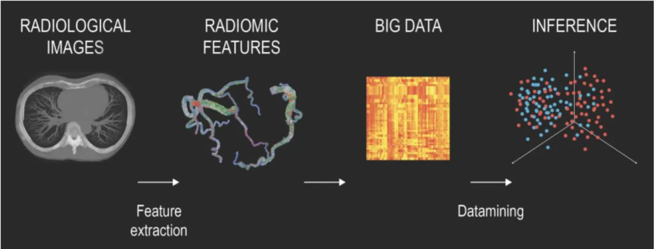
Radiomics is the process of extracting several different features from a given ROI to create large datasets where each abnormality is characterized by hundreds of parameters (24). Some of these parameters are commonly known and used by radiologist, such as the mean attenuation value or the longest diameter of a lesion, while others that quantify the heterogeneity or shape of an abnormality are less apparent. From these values novel analytical methods are used to identify connections between the parameters and the clinical or outcome data. Datamining is the process of finding new meaningful patterns and relationships between numerous variables. From these results, novel imaging biomarkers can be identified which could increase the diagnostic accuracy of radiological examinations and expand our knowledge of the underlying pathological processes (figure 5).

(21)

Figure 5. Pipeline of radiomics-based patient analysis (24).

After image acquisition, new novel radiomics-based image characteristics are extracted to quantify different lesion properties. The hundreds of variables are joined together to create ‘big data’ databases. Datamining is used to find new meaningful connections between the parameters and the clinical outcome data. Based on the results, new imaging biomarkers can be identified which have the potential to increase the diagnostic accuracy of radiological examinations.

Coronary lesions are complex pathologies made up of several different histological components. These different tissues all absorb radiation to a different extent; thus, they are depicted as having different attenuation values on CT. Basically, each voxel is a separate measurement of how much radiation is absorbed in a given volume, thus CT can be used to evaluate the underlying anatomical structure in vivo. Therefore, it is rational to assume that distinct morphologies of different coronary lesions appear differently on CT.

As a result, numerous qualitative imaging markers have been identified on coronary CTA angiography (18, 22). These characteristics have been shown to be indicators of future MACE (58, 57), but they are prone to inter- and intra-observer variations due to their qualitative nature (112). Therefore, it would be desirable to have quantitative image parameters instead of qualitative markers to express different lesion characteristics.

Radiomics is the specialty of mathematically describing different lesion characteristics

(22)

1.5.1. Intensity-based metrics

Intensity-based metrics are often referred to as first-order statistics, which means that statistics are calculated from the values themselves, not considering any additional information which might be gained from analyzing the relationship of the voxels to each other. These statistics can be calculated by selecting a ROI and extracting the voxel values from it. The values then can be analyzed with the tools of histogram analysis. These statistics can be grouped into three major categories, which quantify different aspects of the distribution: 1) average and spread, 2) shape and 3) diversity.

Most of these statistics are well-known to medical professionals and in some cases are used for describing the characteristics of a coronary lesion. Mean: the value that resembles our values the best, since its distance from all other values is minimal. Median:

the value that divides the distribution into two equal halves. Minimum and maximum:

which are the two extremes of the values. Percentiles: which divide the distribution into a given percent of the data. Interquartile range: which are two specific values which enclose the middle 50% of the data points. These statistics all have to do with average and the spread of the data, they do not convey any information regarding the shape or the diversity of the values themselves. Several different distributions may exist that have the same mean and spread but have very different shapes. Therefore, these statistics are not enough to describe the properties of coronary lesions, since distinct plaque morphologies can have very similar values (figure 6).

The shape of a distribution is commonly described by moments. Moments are a family of mathematical formulas that capture different aspects of the distribution. They are defined as the average of the values (xi) minus a given value (c) raised to a given power (q). If c=the mean (µ) and q=2, then we get the variance, which tells us how spread-out our data is from the mean. If we take the square root of the variance, we receive the standard deviation (SD). In cases of normally distributed data, the SD informs us where approximately 68% of the data is located around the mean. If c=µ and q=3 and we divided our moment by SD³, then we get skewness, which quantifies how asymmetric our distribution is around the mean. Negative skew indicates that a large portion of the data is to the right of the mean, while positive skew means just the opposite. If c=µ and q=4 and we normalize by SD⁴ we receive kurtosis, which enumerates how close our data points are to the mean. Small values indicate that there are few outliers in the data, and

(23)

most values are in one SD distance of the mean, while higher values indicate that a larger proportion of values situated further away from the mean the one SD. In cases of normally distributed data the kurtosis is 3, therefore it is reasonable to compare our kurtosis values to this value to analyze how our values differ as compared to the normal distribution.

Figure 6. Pipeline for calculating first-order statistics on two representative examples of coronary lesions (24).

First the coronary arteries need to be segmented. Then histograms need to be created showing the relative frequency of given Hounsfield-unit values. From these different statistics can be calculated. The image also justifies the use of several different parameters to reflect a lesion, since the average attenuation values and the standard deviations are the same, while only higher moments can differentiate between these two plaques.

(24)

values and is calculated by squaring the relative frequency of the given attenuation values and then summing them. If we only have one type of value then its relative frequency is 1, and therefore uniformity is 1, while if we have several different values, then their probabilities are all smaller than 1 and thus their squared sum will also be smaller than 1.

Entropy is a concept proposed by Shannon in 1948, which measures the information content of our data (113). Events with higher probabilities (p) carry less information since we could have guessed the outcome, while unlikely events carry more information since their occurrence is infrequent thus highlight specific instances. Entropy quantifies uncertainty by weighing the information content of an event with its probability. The entropy of a system is equal to adding up these values and multiplying it by minus 1. The higher the value the more heterogeneous is our data. The amount of entropy is commonly measured in bits.

1.5.2. Texture-based metrics

Previously mentioned parameters discarded all spatial information and only use the absolute values of the voxels themselves, even though we know that the spatial relation of different plaque components has a major effect on plaque vulnerability (38). Plaque composition is expressed by the spatial relationship of the voxels on CTA. This relationship is hard to conceptualize using mathematical formulas. A solution emerged in the 70s, when scientists were presented with the problem of identifying different terrain types from satellite imagery. The field of texture analysis has been evolving ever since.

Texture is the broad concept of describing patterns on images. Patterns are systematic repetitions of some physical characteristic, such as intensity, shape or color. Texture analysis tries to quantify these concepts with the use of mathematical formulas, which are based on the spatial relationship of the voxels.

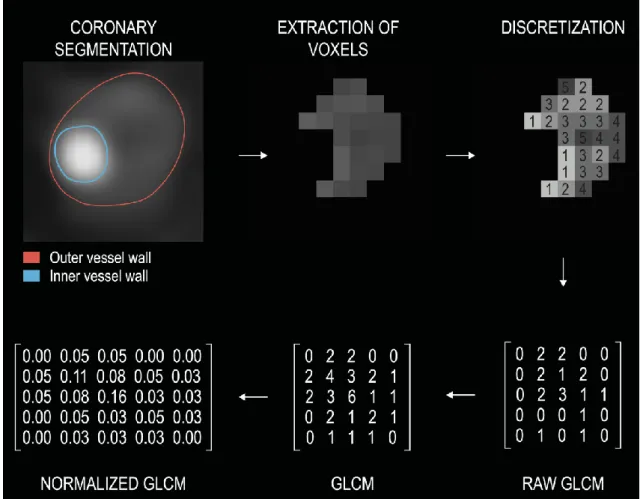
In 1973 Haralick et al. proposed the idea of gray-tone spatial dependencies matrix (GTSDM) commonly known as gray-level co-occurrence matrix (GLCM) for the texture analysis of 2D images. GLCMs are second-order statistics, which means that statistics are calculated from the relationship of 2 pixels’ values, not the values themselves. The goal of these matrices is to quantify how many times similar value voxels are located next to each other in a given direction and distance, and to derive statistics from this information.

(25)

First the coronary arteries need to be segmented to determine the inner and the outer vessel wall boundaries to locate the coronary lesions. Then the HU values of the voxels need to be discretized into a given number of groups, since exactly the same value voxels occur only very rarely in an image. Our GLCM will have exactly the same number of columns as rows, which equals the number of HU groups we discretized our image to.

Next a direction and a distance need to be determined to examine texture. Direction is usually given by an angle. By convention voxels to the east of a reference voxel are at 0˚, ones to the north-east are at 45˚, ones to the north are at 90˚ and ones to the north-west are at 135˚. One only needs to calculate the statistics in these four directions, since the remaining four directions are exact counterparts of these. For example, if our angle equals 0˚ and the distance equals 1, then the raw GLCM is created by calculating the number of times a value j occurs to the right of value i. This number is then put into the i^th row and j^th column of the raw GLCM. If we were to calculate the GLCM in the opposite direction (at 180˚), then we would get very similar results, just that the rows and the columns would be interchanged as compared to the original GLCM (at 0˚), since asking how many times do we find a voxel value j to the right of voxel value i is the same thing as asking how many times will we find a voxel value i to the left of voxel value j. Therefore, for convenience we add the transpose matrix (rows and columns interchanged) to our original raw GLCM matrix to receive a symmetrical GLCM matrix (a value in the i^th row and j^th column equals the value in j^th row and i^th column). Since the absolute numbers are not too informative, we normalize the matrix by dividing all the values in the matrix by the sum of all values in the GLCM to receive relative frequencies instead of absolute numbers.

Pipeline for calculating GLCMs can be found in figure 7.

These matrices contain lot of information on their own. The values on the main diagonal represent the probabilities of finding same value voxels. The further away we move from the main diagonal the bigger the difference between the intensity values. One extreme

(26)

Figure 7. Pipeline for calculating gray-level co-occurrence matrices (24).

First the coronary arteries need to be segmented. Then the voxels need to be extracted from the images. Next the images need to be discretized into n different value groups.

Then a given direction and distance is determined to calculate the GLCM (distance 1, angle 0˚). Raw GLCMs are created by calculating the number of times a value j occurs to the right of value i. This value is then inserted into the i^th row and j^th column of the raw GLCM. To achieve symmetry, the transpose is added to the raw GLCM. Next, the matrix is normalized by substituting each value by its frequency, this results in the normalized GLCM. Afterward, different statistics can be calculated from the GLCMs. To get rotationally invariant results, statistics are calculated in all four directions and then averaged.

GLCM: gray level co-occurrence matrix

Haralick et al. proposed 14 different statistics that can be determined from the GLCMs, but many more exist. All derived metric weight the entries of the matrix by some value depending on what property one wants to emphasize. Angular second moment/uniformity/energy squares the elements of the GLCM and then sums them up.

The fewer the number of different values present in the matrix the higher the value of uniformity. Contrast is calculated by multiplying each value of the GLCM by the difference in the attenuation values squared for that given row and column (i – j)², and

(27)

then adding up all the numbers. We receive bigger weights where there is a large difference between the intensity values of the neighboring voxels, and we receive a weight of 0 for elements on the main diagonal, for cases where the two voxel intensities are equal. Therefore, contrast quantifies the degree of different HU value voxels present in a given direction and distance. Homogeneity/inverse difference moment uses the reciprocal value of the previous weights. This way elements closer to the main diagonal receive higher weights, while values farther away receive smaller values. Since the denominator cannot be 0, thus we add 1 to all weights. Since texture is an intrinsic property of the picture, we should not get different results if we simply rotate our image by 90˚. Therefore, to achieve rotationally invariant results, statistics are calculated on the four GLCMs and then averaged.

While second-order statistics looked at the relationship of two voxels, higher-order statistics assess the relationship of three or more voxels. The easiest concept proposed by Galloway is the gray level run length matrix (GLRLM), which assess how many voxels are next to each other with the same value (114). The rows of the matrix represent the attenuation values, the columns the run lengths. Pipeline for calculating GLRLMs can be found in figure 8.

Galloway proposed 5 different statistics to emphasize different properties of these matrices. Short runs emphasis divides all values by their squared run length and adds them up. Therefore, the number of short run lengths will be divided by a small value, while the number of long run lengths will be divided by a large value, thus short run lengths will be emphasized. Long runs emphasis does just the opposite by instead of dividing the values, it multiplies the entries with the squared run length and then adds them up. Gray level nonuniformity squares the number of run lengths for each discretized HU group and then sums them up. If the run lengths are equally probable in all cases of intensities, then it takes up its minimum. These statistics can also be calculated in all four

(28)

Figure 8. Pipeline for calculating gray level run length matrices (24).

First the coronary arteries need to be segmented. Next the voxels need to be extracted from the images. Then the images need to be discretized into n different value groups.

Next a given direction (angle 0˚) is determined. GLRLMs are created by calculating the number of times a i value voxels occur next to each other in the given direction. The i^th row and jt^h column of the GLRLM represents how many times it occurs in the image, that i value voxels are next to each other j times. To get rotationally invariant results, the statistics calculated in different directions are averaged.

GLRLM: gray level run length matrix

GLCMs and GLRLMs have inspired many to create their own matrices based on some other rule. These are, but not limited to: gray level gap length matrix (115), gray level size zone matrix (116), neighborhood gray-tone difference matrix (117) or the multiple gray level size zone matrix (118).

Laws suggested a different method to emphasize different features of an image (119).

This is done through convolution, which is the multiplication of our voxel values by its neighbors weighted values which results in a new image. Depending on the weights, we can filter out different properties, while emphasizing others. The weights are stored in the kernel matrix. Laws proposed 5 different 1D kernels which emphasize some characteristic, such as ripples or edges. These 1D kernels can be used to create 2 and 3D kernels which can alter radiological images. We can calculate any statistics, for example energy, on these new images to summarize them.

(29)

1.5.3. Shape-based metrics

Atherosclerotic plaques are complex 3D structures situated along the coronary arteries.

The spatial distribution and localization of different plaque components can also have an effect on plaque vulnerability.

1D metrics are based on measuring the distance between 2 points. These parameters are commonly used in clinical practice to describe the magnitude of an abnormality. On coronary CTA the diameter stenosis is used to assess the severity of a lesion, or the length to quantify the extent of a plaque. Diameters measured in different directions can be used to derive new statistics that can resemble some new property, for example the ratio of the longest and the shortest diameter resembles the roundness of a lesion.

2D metrics are calculated on cross-sectional planes and are used to calculate different parameters that are based on areas. These parameters are most often used to approximate some 3D property of the abnormality. The 1D metric diameter and the 2D metric area are all considered approximations of the 3D metric volume. For example, cross-sectional plaque burden is used to approximate full vessel volume-based plaque burden in coronary CTA.

3D metrics try to enumerate different aspects of shape. The geometrical properties of shapes have been thoroughly examined in the field of rigid body mechanics. All objects have so-called principle axes or eigenvectors. These mutually perpendicular axes cross each other at the center of mass. Force applied to these axes act independently, meaning that if we push or rotate the object along on of these principle axes, our object will not move or rotate in any other direction. These eigenvectors also have eigenvalues which can be seen as weights which are proportional to the amount of mass or in our case HU intensity located in that given principle axis. These eigenvectors can be used to quantify different shape-based metrics, for example: roundness, which is the difference between the largest eigenvalues of the smallest enclosing and the largest enclosed ellipse.

(30)

These values can be used to describe the connectedness of different intensity values in the image.

Fractal geometry quantifies self-symmetry by examining repeating patterns at different scales. Objects showing no fractal dimension scale their characteristics exponentially depending on the dimension. For example, if we enlarge a line by 2, its length will increase to 2¹, since it is a 1D object. If we scale one side of a square by 2, then the area of the square will increase by 2² since it is a 2D object. A cube’s volume would increase to 2³ if we were to grow one of its sides by 2. However, fractals act differently. Fractal dimensions do not have to be integers as topological dimensions. In example, the fractal dimension of a line can be anywhere between 1 and 2. This means, if we magnify our line, we see more details that we were not able to see at larger scales. Therefore, if we enlarge a line whose fractal dimension is not equal to its topological dimension, then its length would be more than twice as long. Actually, the length is undefined, since the more we magnify our object the more details we see, therefore this would affect the overall length of the line.

Fractal dimensions measure self-symmetry of objects and quantify how the detail of the object changes as we change our scale (122). Rényi dimensions can be used to calculate fractal dimensions generally. The box-counting dimension or Minkowski–Bouligand dimension is the easiest concept. We calculate how many voxels are occupied by the object. We repeat this at increasing scales. Then we plot the number of voxels containing the object versus the reciprocal of the scale on a log-log plot. The slope of the line will be equal to the box-counting dimension (123, 124).

1.5.4. Transform-based metrics

Images are a vast number of signals arranged in the spatial domain. The images can also be transformed into a different domain, such as the frequency domain, without losing any information. This is basically a different representation of the same information. In the frequency domain the rate at which image intensity values change is used to describe the image instead of assigning intensity values to spatial coordinates.

Fourier transform takes a signal and decomposes it to sinusoidal waves which represent the frequencies present in the signal. Applying the Fourier transform on an image transforms it from the spatial domain to the frequency domain. Gabor transform first

(31)

filters the image by applying a Gaussian-filter before the Fourier transform is performed.

In the frequency domain the images can be filtered from specific components, such as noise, or individual characteristics such as edges can be emphasized or cancelled out.

Using the inverse Fourier transform, we can receive back our modified image in the spatial domain where we can extract different statistics from the filtered image.

Wavelet transform are similar to Fourier transforms in that they also convert the image into the frequency domain, but not all spatial information is lost (125). We can weigh how much frequency and how much spatial information we wish to keep, but we can only increase our spatial information by sacrificing frequency precision, and vice versa. A family of transformed images can be received from different parameter settings, which can be further analyzed using different statistics.

(32)

1.6. Artificial intelligence: the hope to synthetize it all

The increased amount of information can then be analyzed using novel data analytic techniques such as ML and deep learning (DL), which utilize the power of big data to build predictive models, which seek to mimic human intelligence, artificially. These techniques may decrease inter-reader variations, increase the amount of quantitative information and improve the diagnostic and prognostic accuracy, while reducing subjectivity and biases (126).

The amount of available medical information is increasing at exponential speeds (127).

Currently the difficulty is not how to get medical big data, but how to organize, analyze and clinically utilize the data collected in biobanks and repositories. Conventional statistical methods utilize probability theory to create mathematical formulas which describe the relationship between variables. This approach is usually acceptable for population-based analysis, but in the era of precision medicine and big data, new methods are needed which can model complex non-linear relationships and infer results specific to each case rather than being generally true to the population.

Humans are skilled at identifying unique patterns and inferring complex connections between data. However, this natural intelligence is not based on mathematical equations, but on observations and experience. AI tries to create models which think and act humanly and rationally (128). To achieve this, first inputs are needed from the environment. Then this information and the previous observations need to be stored and analyzed, which can be performed using ML. ML is an analytic method a sub-division of AI, which uses computer algorithms with the ability to learn from data, without being explicitly programmed (129). These algorithms are similar to the human learning process, in the sense that more data they are trained on, the better they perform. In the medical field the main goal of ML techniques is to harvest the potential of big data to discover new relationships in the data that conventional statistical methods might not be able to.

While conventional statistical approaches can provide a clear mathematical formula regarding the relationship of the variables, not all methods of ML are capable of describing the connection between parameters through mathematical equations. Instead they build their predictive models based-on patterns in the data experienced through training, and make prediction by comparing a new instance to previous similar

(33)

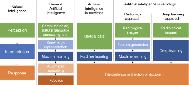
occurrences (130). Nevertheless, ML has the potential to revolutionize medical through providing more accurate predictions of outcomes (figure 9).

Figure 9. Flow diagram showing the possible implementations of artificial intelligence to medical data and showing the similarities and differences between radiomics, machine learning and deep learning (126).

Artificial intelligence tries to mimic natural intelligence through automating processes that are needed for an intelligent system to perceive, interpret and respond to its surroundings. The medical field can utilize the benefits of machine learning to help interpret the large amounts of data currently available in medicine. In case of radiological images, radiomics can be used to extract vast amounts of information, which can be inputs to machine learning. On the other hand, deep learning automatically identifies imaging markers in the neural network while training, rather than defining them beforehand.

(34)

2. OBJECTIVES

2.1. Defining the effect of using coronary CTA to assess coronary plaque burden as opposed to ICA

Even though ICA is considered as the gold-standard of coronary atherosclerosis imagaing, the unique ability of coronary CTA to image atherosclerosis itself may provide the opportunity to identify CAD earlier. Therefore, our objective was to compare coronary CTA and ICA regarding semi-quantitative plaque burden assessment and to assess the effect of imaging modality on cardiovascular risk classification.

2.2. Defining the potential of using radiomics to identify napkin-ring sign plaques on coronary CTA

High-risk plaque morphologies such as the NRS have proven to have additive value in identifying patients vulnerable to MACE. However, the reproducibility of such metrics is poor. As there was no implementation of radiomics to cardiovascular imaging, we sought to assess whether calculation of radiomic features is feasible on coronary lesions.

Furthermore, we aimed to evaluate whether radiomic parameters can differentiate between plaques with or without NRS.

2.3. Defining the potential of radiomics to identify invasive and radionuclide imaging markers of vulnerable plaques on coronary CTA

Invasive imaging modalities due to their better spatial resolution have a better accuracy to identify rupture prone plaques. Furthermore, radionuclide imaging is capable of identifying plaques with inflammation and micro-calcifications which are hallmarks of plaque vulnerability. We wished to assess whether coronary CTA radiomics could outperform current standards to identify invasive and radionuclide imaging markers of high-risk plaques described by intravascular ultrasound (IVUS), optical coherence tomography (OCT) and NaF¹⁸-Positron Emission Tomography (NaF¹⁸-PET).

(35)

2.4. Defining the potential effect of image reconstruction algorithms on reproducibility of volumetric and radiomic signatures of coronary lesions on coronary CTA

Recent advancements in image reconstruction have led to the wide-spread utilization of novel iterative reconstruction techniques. As volumetric and radiomics features are calculated from the voxel values themselves, it is important to know how these may change the calculated metric values. Therefore, our primary aim was to assess whether filtered back projection (FBP), hybrid (HIR) or model-based (MIR) iterative reconstruction have any significant effect on volumetric and radiomic parameters of coronary plaques. Furthermore, we sought to evaluate the impact of the type of binning and the number of bins used for discretization on radiomic parameter values.

2.5. Defining the potential of using radiomic markers as inputs to machine learning models to identify advanced atherosclerotic lesions as assessed by histology

The plaque attenuation pattern scheme outperforms conventional plaque classification to identify advanced atherosclerotic lesions. Recently, quantitative histogram analysis and the area or volume of low attenuation plaque have been proposed as markers of high-risk lesions. Furthermore, radiomics represents a process of extracting thousands of imaging markers from radiological images describing the heterogeneity and spatial complexity of lesions. These quantitative features can be used as the input to ML. Therefore, our objective was to compare the diagnostic performance of radiomics-based ML with visual and histogram-based plaque assessment to identify advanced coronary lesions using histology as reference standard.

(36)

3. METHODS

3.1. Study design and statistics for defining the effect of using coronary CTA to assess coronary plaque burden as opposed to ICA

The Genetic Loci and the Burden of Atherosclerotic Lesions study enrolled patients who were referred to coronary CTA due to suspected CAD (NCT01738828). Detailed description of the patient population, including the inclusion and exclusion criteria, has been published (131). This ancillary study was designed as a nested single-center observational cohort study in patients who were referred to ICA due to obstructive CAD detected by CTA. The study was approved by the Institutional Ethical Review Board, and all participants provided written informed consent (131).

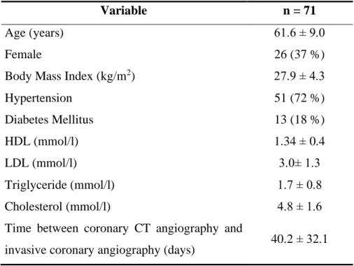
Out of the 868 patients enrolled by our institution, we selected individuals who underwent both coronary CTA and ICA within 120 days. In total, 71 patients (mean age 61.6±9.0 years, 36.6% female) were included in our analysis. In 58 patients, ICA followed CTA based on clinical findings, while in 13 cases ICA was carried out before CTA. These patients were either referred to CTA after revascularization due to atypical chest pain (7 patients) or were referred to left atrial angiography before radiofrequency ablation (6 patients). An average of 40.2 days passed between the two examinations.

All images were randomly and independently analyzed. Semi-quantitative plaque burden quantification of ICA images was performed by an interventional cardiologist. A minimum of 5 projections of the left and right coronary systems were acquired in each patient. All coronary segments were analyzed blinded to CTA results, using a minimum of 2 projections. Coronary CTA images were analyzed by a cardiologist.

A total of 1016 segments were assessed based on the 18-segment SCCT classification with both modalities (132). We excluded 16 segments due to presence of coronary stents leading to overall 1000 analyzed segments. All segments were scored for the presence or absence of plaque (0: Absent; 1: Present) and the degree of stenosis (0: None; 1: Minimal (<25%); 2: Mild (25%-49%); 3: Moderate (50%-69%); 4: Severe (70%-99%) or 5:

Occlusion (100%)). In case multiple lesions were present in a segment, the observers recorded the highest degree of stenosis for that segment. In each patient, segment involvement score (SIS) was used to quantify the number of segments with any plaque,

(37)

whereas segment stenosis score (SSS) was calculated by summing the stenosis scores of each segment. Indexed values were calculated by dividing the SIS and SSS scores by the number of segments: segment involvement score index (SISi) = SIS / number of segments; segment stenosis score index (SSSi) = SSS / number of segments.

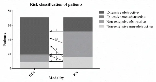
Based on Bittencourt et al. the extent of CAD was classified as non-extensive (SIS ≤ 4) or extensive (SIS > 4) and obstructive (at least one segment with ≥50% stenosis) or nonobstructive (no segment with ≥50% stenosis).(133) Patients were classified as extensive obstructive, nonextensive obstructive, extensive nonbostructive or nonextensive nonobstructive based on ICA and also CTA results.

All continuous variables are expressed as mean ± SD, while categorical variables are expressed as frequencies and percentages. Presence of plaque was compared using the chi-square test between modalities. Sensitivity, specificity, positive predictive value and negative predictive value were calculated to assess the diagnostic accuracy of CTA as compared to ICA as reference standard. SIS, SSS and SISi, SSSi were compared using the paired t-test between modalities. Reclassification rate was calculated by dividing the number of people who shifted groups based on the two modalities by the total study population. All statistical calculations were performed using SPSS software (SPSS version 23; IBM Corp., Armonk, NY). A p-value of 0.05 or less was considered significant.

(38)

3.2. Study design and statistics for defining the potential of using radiomics to identify napkin-ring sign plaques on coronary CTA

From 2674 consecutive coronary CTA examinations due to stable chest pain we retrospectively identified 39 patients who had NRS plaques. Two expert readers reevaluated the scans with NRS plaques. To minimize potential variations due to inter- reader variability the presence of NRS was assessed using consensus read. Readers excluded 7 patients due to insufficient image quality and 2 patients due to the lack of the NRS, therefore 30 coronary plaques of 30 patients (NRS group; mean age: 63.07 years [interquartile range (IQR): 56.54; 68.36]; 20% female) were included in our analysis. As a control group, we retrospectively matched 30 plaques of 30 patients (non-NRS group;

mean age: 63.96 years [IQR: 54.73; 72.13]; 33% female) from our clinical database with excellent image quality. To maximize similarity between the NRS and the non-NRS plaques and minimize parameters potentially influencing radiomic features, we matched the non-NRS group based on degree of calcification and stenosis, plaque localization, tube voltage and image reconstruction.

All plaques were graded for luminal stenosis and degree of calcification. Furthermore, plaques were classified as having low attenuation if the plaque cross-section contained any voxel with <30 HU and having spotty calcification if a <3 mm calcified plaque component was visible.

Image segmentation and data extraction was performed using a dedicated software tool for automated plaque assessment (QAngioCT Research Edition; Medis medical imaging systems bv, Leiden, The Netherlands). After automated segmentation of the coronary tree the proximal and distal end of each plaque were set manually. Automatic lumen and vessel contours were manually edited by an expert if needed (134). From the segmented datasets 8 conventional quantitative metrics (lesion length, area stenosis, mean plaque burden, lesion volume, remodeling index, mean plaque attenuation, minimal and maximal plaque attenuation) were calculated by the software. The voxels containing the plaque tissue were exported as a DICOM dataset using a dedicated software tool (QAngioCT 3D workbench, Medis medical imaging systems bv, Leiden, The Netherlands). Smoothing or interpolation of the original HU values was not performed. Representative examples of

(39)

volume rendered and cross-sectional images of NRS and non-NRS plaques are shown in figure 10.

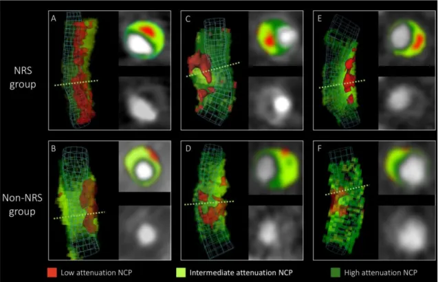
Figure 10. Representative images of plaques with or without the napkin ring sign (135).

Volume rendered and cross-sectional images of plaques with napkin-ring sign in the top row (A, C, E) and their corresponding matched plaques in the lower row (B, D, E). Green dashed lines indicate the location of cross-sectional planes. Colors indicate different CT attenuation values.

NCP: non-calcified plaque; NRS: napkin-ring sign

We developed an open source software package in the R programing environment (Radiomics Image Analysis (RIA)) which is capable of calculating hundreds of different radiomic parameters on 2D and 3D datasets (136). We calculated 4440 radiomic features for each coronary plaque using the RIA software tool. Detailed description on how

(40)

analysis and calculated area under the curve (AUC) with bootstrapped CI values using 10,000 samples with replacement and calculated sensitivity, specificity, positive and negative predictive value by maximizing the Youden index (138). To assess potential clusters among radiomic parameters, we conducted linear regression analysis between all pairs of the calculated 4440 radiomic metrics. The 1-R² value between each radiomic feature was used as a distance measure for hierarchical clustering. The average silhouette method was used to evaluate the optimal number of different clusters in our dataset (139).

Furthermore, to validate our results we conducted a stratified 5-fold cross-validation using 10,000 repeats of the three best radiomic and conventional quantitative parameters.

The model was trained on a training set and was evaluated on a separate test set at each fold using ROC analysis. The derived curves were averaged and plotted to assess the discriminatory power of the parameters. The number of additional cases classified correctly was calculated as compared to lesion volume. The McNemar test was used to compare classification accuracy of the given parameters as compared to lesion volume (140). Due to the large number of comparisons, we used the Bonferroni correction to account for the family wise error rate. Bonferroni correction assumes that the examined parameters are independent of each other, thus the question is not how many parameters are being tested, but how many independent statistical comparisons will be made.

Therefore, based on methods used in genome-wide association studies we calculated the number of informative parameters accounting for 99.5% of the variance using principal component analysis (141, 142). Overall, 42 principal components identified, therefore p values smaller than 0.0012 (0.05/42) were considered significant. All calculations were done in the R environment (143).

Characterization of coronary atherosclerosis on computed tomography using advanced image processing techniques