Abdominal and Pericoronary Adipose Tissue Quantification with Computed Tomography and
Their Relationship to Cardiovascular Risk Factors and Inflammatory Markers
Ph.D. Thesis
Pál Maurovich Horvat M.D.
Semmelweis University
Doctoral School of Basic Medical Sciences
Supervisor: Béla Merkely M.D., Ph.D., D.Sc.
Official Reviewers: Pál Pánczél M.D., Ph.D.
Attila Thury M.D., Ph.D.
Head of the Comprehensive Exam Committee:
Péter Kempler M.D., Ph.D., D.Sc
Members of the Comprehensive Exam Committee:
Károly Cseh M.D., Ph.D., D.Sc Tibor Hídvégi M.D., Ph.D.
Budapest 2011
Table of Content
Abreviations... 5
1 Introduction ... 6
1.1 Abdominal adipose tissue compartment ... 7
1.2 Pericoronary adipose tissue compartment ... 10
2 Aims ... 12
2.1 Planimetric and volumetric adipose tissue quantification methods ... 12
2.2 Abdominal adipose tissue volumes and metabolic risk factors ... 12
2.3 Abdominal adipose tissue volumes and markers of inflammation and oxidative stress ... 12
2.4 Novel volumetric pericoronary adipose tissue quantification ... 13
3 Methods ... 13
3.1 Study population ... 13
3.1.1 Framingham Heart Study ... 13
3.1.2 ROMICAT study ... 15
3.2 Abdominal adipose tissue assessment ... 15
3.2.1 MDCT scan protocol for abdominal adipose tissue quantification ... 15
3.2.2 Measurements of abdominal adipose tissue areas and volumes ... 15
3.2.3 Measurements of sagital diameter and waistline ... 16
3.2.4 Reproducibility ... 16
3.2.5 Risk factor and covariate assessment ... 17
3.2.6 Biomarker assessment ... 18
3.3 Pericoronary adipose tissue assessment ... 18
3.3.1 MDCT scan protocol for pericoronary adipose tissue quantification ... 18
3.3.2 Pericoronary adipose tissue volumetric assessment ... 19
3.3.3 Coronary artery plaque assessment ... 21
3.3.4 Hs-CRP assessment ... 21
3.4 Statistical analysis ... 22
3.4.1 Abdominal fat quantification reproducibility study: Statistical considerations ... 22
3.4.2 Abdominal adipose tissue and metabolic risk factors: Statistical considerations ... 22
3.4.3 Abdominal adipose tissue and markers of inflammation: Statistical considerations ... 23
3.4.4 Pericoronary adipose tissue quantification: Statistical considerations ... 24
4 Results ... 26
4.1.1 The reproducibility study ... 26
4.1.2 Intra-observer variability ... 26
4.1.3 Inter-observer variability ... 28
4.1.4 Ratio of subcutaneous and visceral adipose tissue volumes ... 29
4.1.5 Relation of volumetric based adipose tissue measurements to WL, SD, and BMI ... 30
4.1.6 Abdominal adipose tissue distribution by age and sex ... 31
4.2 The abdominal adipose tissue depots and metabolic risk factors ... 31
4.2.1 Correlations with SAT and VAT ... 33
4.2.2 Multivariable-adjusted regressions with SAT, VAT, and metabolic risk factors ... 34
4.2.3 Residual effect of VAT in multivariable models that contain BMI and WL ... 36
4.2.4 Risk factor distribution based on quartiles of VAT ... 39
4.3 Abdominal adipose tissue depots and the markers of inflammation and oxidative stress ... 40
4.3.1 Correlations with SAT and VAT ... 41
4.3.2 Multivariable-adjusted regressions with SAT and VAT ... 42
4.3.3 Multivariable-adjusted regressions with Both SAT and VAT in models ... 44
4.3.4 Addition of SAT and VAT to multivariable models that included BMI and WL ... 45
4.3.5 Secondary analyses ... 45
4.4 Pericoronary adipose tissue quantification ... 50
4.4.1 Reproducibility of PCAT measurements ... 51
4.4.2 Patient based PCAT analysis ... 51
4.4.3 Vessel based PCAT analysis ... 53
4.4.4 Subsegment based PCAT analysis ... 53
5 Discussion... 55
5.1.1 Abdominal adipose tissue, metabolic risk and inflammation... 55
5.1.2 Pericoronary adipose tissue quantification ... 64
5.1.3 Strengths and limitations ... 66
6 Conclusions ... 67
7 Summary ... 69
8 Összefoglalás ... 70
9 References ... 71
10 Publications ... 86
10.1 Publications closely related to the present thesis ... 86
10.2 Publications not related to the present thesis ... 88
Acknowledgement ... 94
Appendix (Papers 1-3) ... 95
Abreviations
ANOVA Analysis of Variance BMI Body Mass Index
CT Computed Tomography
CVD Cardiovascular Disease EAT Epicardial Adipose Tissue FFA Free Fatty Acids
HDL High Density Lipoprotein
hs-CRP High Sensitivity C-reactive Protein
HU Hounsfield Unit
ICAM-1 Intercellular Adhesion Molecule-1 ICC Intra-class Correlation Coefficient IL-6 Interleukin-6
IQR Inter Quartile Range
LAD Left Anterior Descendent Coronary Artery LCx Left Circumflex Coronary Artery
LM Left Main Coronary Artery
Lp-PLA2 Lipoprotein Associated Phospholipase A2 MCP-1 Monocyte Chemoattractant Protein-1 MDCT Multidetector-row Computed Tomography MetS Metabolic Syndrome
MRI Magnetic Resonance Imaging PAI-1 Plasminogen Activator Inhibitor PCAT Pericoronary Adipose Tissue RCA Right Coronary Artery
SAT Subcutaneous Adipose Tissue SD Standard Deviation
SAA Subcutaneous Adipose Tissue Area SAV Subcutaneous Adipose Tissue Volume TNF-α Tumor Necrosis Factor Alpha
VAT Visceral Adipose Tissue VAA Visceral Adipose Tissue Area VAV Visceral Adipose Tissue Volume WHO World Health Organization
WL Waistline
1 Introduction
Cardiovascular disease (CVD) is the leading cause of morbidity and mortality in the industrialized countries (1). Improvements in CVD risk factor profiles have led to significant reductions in death from CVD over the past 50 years (2), but recent data suggest that the increasing prevalence of obesity may have slowed this rate of decline (3).
The prevalence of obesity is beginning to exceed the prevalence of undernutrition and infectious diseases in several developing countries, which means that the full impact of the obesity epidemic has yet to be realized (4-8).
Furthermore, obesity increases the risk to develop less well-known complications, which include certain types of cancer, hepatic steatosis, gallbladder disease, respiratory complications (obstructive sleep apnea), endocrine abnormalities, obstetric complications, trauma to the weight-bearing joints, gout, cutaneous disease, proteinuria, increased hemoglobin concentration, and possibly immunologic impairment (9).
Epidemiological studies and life-insurance data confirm that increasing degrees of overweight are important predictors of decreased longevity (10). In the Framingham Heart Study, the risk of death within 26 years increased by 1% for each extra 0.45 kilogram increase in weight between the ages of 30 years and 42 years, and by 2%
between the ages of 50 years and 62 years (11).
In clinical practice and in epidemiological studies the body fatness is most commonly estimated by the body-mass index (BMI), which represents weight in kilograms divided by the square of the height in meters (12). The World Health Organization (WHO) expert committee proposed the classification of overweight and obesity which applies to all adult age groups (Table 1.) (13,14).
Table 1 - Cut-off points proposed by a WHO expert committee for the classification of overweight
BMI (kg.m-2) WHO classification Popular description
<18,5 Underweight Thin
18,5-24,9 - “normal”, “acceptable”
25,0-29,9 Grade 1 overweight Overweight
30,0-39,9 Grade 2 overweight Obesity
≥40,0 Grade 3 overweight Morbid obesity
The main assumption behind the BMI as a metric of adiposity is that most variation in weight for persons of the same height is due to fat mass. The graded classification of overweight using BMI values provides valuable information about increasing body fatness. Body mass index allows useful comparisons of weight within and between populations and the identification of individuals and groups at highest risk of morbidity and mortality. However, it is important to appreciate that, owing to differences in body proportions, BMI may not correspond to the same degree of fatness across different populations. Nor does it account for the wide variation in the nature of obesity between different individuals and populations (12).
Despite these shortcomings in the calculation the relationship between BMI and the incidence of several chronic conditions caused by excess fat is approximately linear for a range of BMI indexes less than 30 kg m-2, but all risks are greatly increased for those subjects with a BMI above 29 kg m-2, independent of gender (15,16).
1.1 Abdominal adipose tissue compartment
Despite all of the health hazards of obesity there are some very obese patients without any complications and with fairly normal metabolic risk profile. On the other hand, there are some moderately obese patients who develop multiple metabolic and atherogenic abnormalities. It was previously demonstrated that, for a given BMI or total amount of body fat, the subgroup of patients with excessive intra-abdominal, or visceral adipose
tissue depot is at substantially higher risk of developing insulin resistance and metabolic syndrome (17).
In the mid-twentieth century, Jean Vague, a French physician, made an important clinical observation that went largely unnoticed at the time. He described that body fat distribution, rather than excess body weight per se, was one of the key components associated with the presence of diabetes mellitus and CVD (18). Even at that time, he had suggested the concept that android obesity (upper body obesity) was associated with the risk of developing metabolic dysfunction conditions such as diabetes, CVD, and gout.
During the past two decades it became clear that, different ectopic fat compartments may be associated with differential metabolic risk (19). Several metabolic studies demonstrated that central type of obesity pose a greater risk for developing obesity- related disorders than BMI alone (20,21). In particular, the visceral adipose tissue (VAT) compartment may be a unique pathogenic fat depot (21-23). Visceral adipose tissue has been termed an endocrine organ, in part because it secretes adipocytokines and other vasoactive substances that can influence the risk of developing metabolic traits (23-26). It has been further emphasized by many metabolic investigations that excess visceral adiposity is a key feature of a phenomenon referred to as ectopic fat deposition, which has been connected to a plethora of metabolic dysfunctions (27). Available studies report relations of greater subcutaneous adipose tissue (SAT) and VAT with a higher prevalence of impaired fasting glucose (21,28), diabetes (21,23,29), insulin resistance (21,30,31), hypertension (32-34), atherogenic dyslipidemia (35-39), impaired fibrinolysis/increased risk of thrombosis and inflammation (40-42). It should be emphasized that these metabolic features, most commonly found in the viscerally obese patient, are often referred as the metabolic syndrome, which is linked to the development of cardiovascular disease (CVD). The metabolic syndrome of visceral obesity has been described as a
“multiplex” additional modifiable CVD risk factor that - when added to traditional risk factors determines global “cardiometabolic risk” (43,44).
Inflammation is one of the important factors in the development of CVD and associated adverse clinical events (45). In the past decade, it became clear that chronic low-grade inflammation, such as is encountered in individuals with an excess of visceral/ectopic fat plays an important role in several cardiovascular disorders (46). In terms of its
proinflammatory and metabolic features, visceral adiposity is an emergent powerful but modifiable risk factor for CVD. Therefore, the precise and reproducible quantification of ectopic fat depots is important in order to further characterize the role of adipose tissue in the development of cardiovascular disorders.
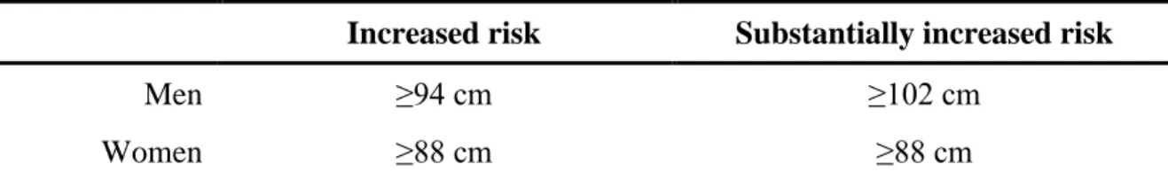
Waist circumference measurement is widely used in clinical practice to assess abdominal obesity (47). The waistline (WL) correlates with measures of risk for coronary heart disease such as hypertension or blood lipid levels. The choice of cut-off points on the waist circumference continuum involves a trade-off between sensitivity and specificity similar to that for BMI. Gender-specific cut-off points for waist circumference may be of guidance in interpreting values for adults: proposed cut-off levels are shown in Table 2, with level 1 being intended to alert clinicians to potential risk, whereas level 2 should initiate therapeutic action (48). Waistline measurement is easily obtainable, however it is important to note that it is an imprecise measure of abdominal adiposity (49) because it is a function of both the SAT and VAT compartments. Therefore, assessment of VAT requires imaging with radiographic techniques such as computed tomography (CT) or magnetic resonance imaging (MRI).
Table 2 – Waistline predicts risk of metabolic complications
Increased risk Substantially increased risk
Men ≥94 cm ≥102 cm
Women ≥88 cm ≥88 cm
Gender-specific waistlines are presented as “increased risk” (level 1) and “substantially increased risk”
(level 2) of metabolic complications associated with obesity in Caucasian population.
Current imaging studies evaluating abdominal fat depots are limited to small, referral- based samples often enriched for adiposity-related traits (33,35-37,50-52). Furthermore, study samples have often been limited to either women or men, precluding the study of sex differences (32,33,35-38,52,53). Some studies have focused on Japanese Americans or Southeast Asians (29,32,36,39,53,54), ethnic groups with more visceral fat than expected for a given overall BMI (55).
Multidetector-row CT permits highly reproducible volumetric measurements of both SAT and VAT (56). In addition, this initial observation suggested that volumetric fat measurements - as opposed to previous studies using single-slice methodology - can accurately characterize the heterogeneity of abdominal fat distribution between individuals and the differences in fat distribution with age and between women and men.
Furthermore, no data is available in a community-based sample of women and men free of CVD across the spectrum of BMI whether the volume of SAT (subcutaneous adipose tissue volume, SAV) and VAT (visceral adipose tissue volume, VAV) are associated with metabolic risk factors and markers of inflammation cross-sectionally. It is not fully understood whether VAT is more strongly associated with metabolic risk factors than is SAT.
1.2 Pericoronary adipose tissue compartment
Recently, an influence of thoracic adipose tissue on the development of coronary artery disease (CAD) has been suggested, as it has been shown that pericardial fat is closely associated with cardiovascular risk factors and cardiovascular disease (57,58). Epicardial adipose tissue (EAT) covers 70-100% of the cardiac circumference as a layer of adipose tissue between the myocardium and the visceral pericardium (59). Notably, EAT and intra-abdominal fat originate from the same visceral white preadipocytes during embryogenesis and both are rich source of bioactive molecules (60). EAT secretes several pro- and anti-inflammatory mediators such as tumor necrosis factor-alpha (TNF- α), interleukine-6 (IL-6), free fatty acids (FFA), plasminogen activator inhibitor-1 (PAI- 1), and adipocytokines such as adiponectin (61-63). It has been suggested that adipocytokines produced by fat surrounding the coronary arteries might amplify vascular inflammation and generate a pro-atherogenic processes in the vessel wall from „outside- to-inside‟ (64,65). Elevated pericardial fat volumes may lead to a mismatch in the production of pro- and anti-inflammatory mediators (66). The portion of EAT which directly surrounds the coronary arteries is termed as pericoronary adipose tissue (PCAT).
The pericoronary adipose tissue compartment may have a key role in the development of
coronary artery disease through a paracrine effect that causes amplification of inflammation, plaque instability, and neovascularization (24).
The precise and reproducible quantification of this rather small, pericoronary visceral fat compartment is crucial for the understanding of its role in coronary artery atherogenesis.
The most commonly used techniques for PCAT quantification in cardiac computed tomography (CT) datasets are based on thickness and area measurements on a limited number of axial image slices (65,67-69). Recent studies reported a moderate to poor reproducibility of the PCAT thickness and area measurements, with a reported coefficient of variation between 12.0% - 23.4% and intra-class correlation coefficient of 0.76 (95%
CI 0.50 – 0.88) (65,67,68). Moreover, these 2-dimensional quantification techniques do not reflect the inhomogeneous distribution of PCAT along the atrioventricular and interventricular grooves due to the limitations posed by the single CT cross-sectional assessment.
There is no three-dimensional, threshold based quantification method available for PCAT assessment. The few available studies have used PCAT thickness measurement in single slices and reported contradictory results regarding the relationship between the severity of coronary atherosclerosis and PCAT quantity (67,68). Furthermore, it is not fully understood whether PCAT is a marker of overall adiposity or an independent pathogenic fat depot.
We hypothesize that precise and reproducible three-dimensional quantification of PCAT could provide insights into the pathophysiological role of this distinct adipose tissue depot in coronary atherosclerotic plaque development.
2 Aims
2.1 Planimetric and volumetric adipose tissue quantification methods
We sought to assess the intra- and inter-observer reproducibility of MDCT based volumetric quantification of subcutaneous and visceral abdominal adipose tissue.
Furthermore, our aim was to investigate the differences between the relative amounts of visceral and subcutaneous abdominal tissue quantity as assessed by volumetric and planimetric methods. In addition, we investigated the relation of MDCT based measurements to anthropometric measures of obesity such as BMI, sagital diameter (SD) and waistline (WL).
2.2 Abdominal adipose tissue volumes and metabolic risk factors
We aim to assess whether the volume of SAT and VAT are associated with metabolic risk factors in a community-based sample free of CVD. Furthermore, we sought to determine whether sophisticated volumetric imaging methods of SAT and VAT provide information about metabolic risk other than that offered by classic anthropometric measures such as BMI and WL.
2.3 Abdominal adipose tissue volumes and markers of inflammation and oxidative stress
We aim to investigate the association of abdominal fat compartment volumes with a panel of systemic inflammatory markers. Furthermore, we sought to assess whether volumetric measurements of SAT and VAT explained additional interindividual variability in biomarker concentrations above that accounted for by the simple clinical anthropometric measures of obesity BMI and WL.
2.4 Novel volumetric pericoronary adipose tissue quantification
Cardiac computed tomography (CT) allows for simultaneous assessment of PCAT volume and coronary artery plaque. Volumetric quantification of PCAT in patients with and without CAD in conjunction with high and low hs-CRP levels could provide insights into the pathophysiological role of this distinct adipose tissue depot and its local effect on coronary atherosclerosis. Thus, we aimed to 1) assess the feasibility and reproducibility of a novel threshold-based method of PCAT volume quantification using cardiac CT, 2) determine the relationship of PCAT volume to the presence of coronary atherosclerotic plaque on patient, vessel and subsegment basis. We have examined the surrounding PCAT volume in groups of patients with presence of coronary plaque and high hs-CRP and no plaque and low hs-CRP levels, furthermore we have investigated a third intermediate group with no plaque and high hs-CRP level.
3 Methods
3.1 Study population
3.1.1 Framingham Heart Study
Participants for this study were drawn from the Framingham Heart Study Multidetector Computed Tomography Study, a population-based substudy of the community-based Framingham Heart Study Offspring and Third-Generation Study cohorts. Beginning in 1948, 5209 men and women 28 to 62 years of age were enrolled in the original cohort of the Framingham Heart Study. The offspring and spouses of the offspring of the original cohort were enrolled in the Offspring Study starting in 1971. Selection criteria and the original study design have been described elsewhere (70,71). Beginning in 2002, 4095 Third Generation Study participants, who had at least 1 parent in the offspring cohort, were enrolled in the Framingham Heart Study and underwent standard clinic
examinations. The standard clinic examination included a physician interview, a physical examination, and laboratory tests. For the present study, the study sample consisted of Offspring and Third Generation Study participants who were part of the multidetector- row CT substudy.
Between June 2002 and April 2005, 3529 participants (2111 third generation, 1418 offspring participants) underwent multidetector-row CT assessment of coronary and aortic calcium. Inclusion in this study was weighted toward participants from larger Framingham Heart Study families and those who resided in the greater New England area. Overall, 755 families were included in our analysis. Men had to be ≥35 years of age; women had to be ≥40 years of age and not pregnant; and all participants had to weigh <160 kilograms. Of the participants, 433 (222 offspring and 211 third generation) were imaged as participants in an ancillary study using an identical imaging protocol, the National Heart, Lung, and Blood‟s Family Heart Study (72). Of the total 3529 subjects imaged, 3394 had interpretable CT measures; of those, 3329 had both SAT and VAT measured; of those, 3124 of them were free of CVD; of those, 3102 attended a contemporaneous examination; and of those, 3001 had a complete covariate profile.
Thus, the overall sample size for analysis is 3001.
The biomarkers and inflammatory substances were assessed in the offspring participants with technically interpretable CT scans (n=1377), attendance at the seventh examination cycle (1998-2001; n=1355), complete covariate information (n=1253), and measurement of at least one inflammatory marker, resulting in a total sample size of 1250 participants.
Sample size varied slightly for individual markers; TNF-α and isoprostane measurements were only available on a subset (n=920 and 1010, respectively). The CT scan was performed an average of 4.2 years after the seventh examination cycle (when covariates and inflammatory markers were measured).
The study was approved by the institutional review boards of the Boston University Medical Center and Massachusetts General Hospital, Harvard Medical School. All subjects provided written informed consent.
3.1.2 ROMICAT study
From May 2005 to May 2007 consecutive subjects were prospectively enrolled as part of the ROMICAT (Rule Out Myocardial Infarction using Computer Assisted Tomography) trial. Details of the study have been previously reported (73). From the 368 ROMICAT patients, we included 51 patients in this age- and gender-matched 1:1:1 case-control design. Patients were stratified into 3 groups based on presence of coronary atherosclerosis and hs-CRP levels. Group 1 included patients with presence of coronary plaque and hs-CRP >2.0 mg/L; intermediate group (Group 2) included patients with no plaque and hs-CRP >2.0 mg/L, Group 3 included patients with no plaque and hs-CRP
<1.0 mg/L. The hs-CRP cutoff points were selected according to data from recent clinical trials and scientific statements (74-76). We included only patients with right coronary artery (RCA) dominance or co-dominance to avoid potential bias due to small RCA in coronary systems with left dominance.
3.2 Abdominal adipose tissue assessment
3.2.1 MDCT scan protocol for abdominal adipose tissue quantification
All subjects underwent CT scanning in a supine position using an eight-slice MDCT (LightSpeed Ultra, General Electric, Milwaukee, WI, USA). Twenty-five contiguous 5 mm thick slices (120 kVp, 400 mA, gantry rotation time 500 ms, table feed 3:1) were acquired covering 125 mm above the level of S1. The raw data were reconstructed using a 55 cm field of view. The effective radiation exposure was 2.7 mSv.
3.2.2 Measurements of abdominal adipose tissue areas and volumes
We measured the subcutaneous and visceral adipose tissue areas (SAA and SAA) and volumes (SAV and SAV) as well as the waistline (WL) and sagital diameter (SD) using a
dedicated offline workstation (Aquarius 3D Workstation, TeraRecon Inc., San Mateo, CA, USA). The SAA (cm2) and SAA (cm2) as well the WL (cm) and SD (cm) were measured using a single slice (5 mm thickness) at the umbilical level (77,78). In CT absolute Hounsfield units (HU) of pixels correspond directly to the tissue property. Thus, we applied predefined image display setting to determine the visceral and subcutaneous adipose tissue areas using a window width of -195 to -45 HU and a window center of - 120 HU to identify pixels containing adipose tissue (79,80). In order to separate visceral from subcutaneous adipose tissue the abdominal muscular wall separating the two compartments was manually traced.
The SAV and VAV were measured across the total imaging volume and were calculated in cm3. We applied a semi-automatic segmentation technique using the same image display settings as for the area measurements. The abdominal muscular wall separating the two adipose tissue compartments was manually traced in four sections of the imaging volume representing the quartiles of the scanning range (1st, 9th, 17th, and 25th slice).
The segmentation of the entire scanning volume was performed automatically interpolating the information of the manually defined traces. If necessary, manual adjustments were made throughout the scan volume. The average time for image analysis was 5 minutes per subject.
3.2.3 Measurements of sagital diameter and waistline
The sagital abdominal diameter (SD) and the waistline (WL) were measured at the level of the umbilicus. The SD (cm) was defined as the shortest distance between the mid- anterior wall of the abdomen and the mid-posterior wall. The WL (cm) was directly measured by tracing the circumference of the abdominal skin.
3.2.4 Reproducibility
The reproducibility study sample represents a random subset of 100 Caucasian subjects (age range: 37 – 83 years; 49% female) drawn from the offspring cohort, who underwent MDCT scanning (n = 1418). The random sample was taken to ensure approximately
equal number of men and women, and an approximately equal number of participants in each of the age groups of 35-44, 45-54, 55-64, 65-74 and 75-84 years, were represented (approximately 10 per age group per sex).
Two observers performed an independent analysis of all datasets in random order to assess for inter-observer variability. One reader repeated the analysis one week later to assess for intra-observer variability.
3.2.5 Risk factor and covariate assessment
Risk factors and covariates were measured at the contemporaneous examination. BMI was measured at each index examination, and standing WL, obtained at the level of the umbilicus, were measured by trained technicians following written protocols. Fasting plasma glucose, total and high-density lipoprotein (HDL) cholesterol, and triglycerides were measured on fasting morning samples. Diabetes was defined as a fasting plasma glucose level ≥126 mg/dL at a Framingham examination or treatment with either insulin or a hypoglycemic agent. Hypertension was defined as systolic blood pressure of at least 140 mmHg or diastolic blood pressure of at least 90 mmHg or current antihypertensive treatment. Prevalent cardiovascular disease was defined at the seventh examination cycle as coronary heart disease, stroke, heart failure, or intermittent claudication as described previously (81). Chronic aspirin use was defined as self-reported aspirin use three or more times/week. Participants were considered current smokers if they had smoked at least 1 cigarette per day for the previous year. Assessed through a series of physician- administered questions, alcohol use was dichotomized on the basis of consumption of
>14 drinks per week (in men) or 7 drinks per week (in women). Physical activity, determined by questionnaire, was represented as the weighted sum of the proportion of a typical day spent sleeping and performing sedentary, slight, moderate, or heavy physical activities (82). Post-menopausal status was defined as cessation of menses for at least one year. Impaired fasting glucose was defined as a fasting plasma glucose level of 100 to 125 mg/dL among those not treated for diabetes. Metabolic syndrome (MetS) was defined from modified Adult Treatment Panel criteria (83).
3.2.6 Biomarker assessment
Biomarkers were measured on fasting morning samples collected at the participant‟s visit during the seventh examination cycle (1998-2001) as previously described (84). Samples were stored at -80ºC and thawed at the time of analysis (with exception of urine, see below). Serum CRP serum was measured by high-sensitivity assay [(Dade Behring BN100 nephelometer; mean intra-assay CV 3.2%]. Fibrinogen was measured in duplicate from citrated plasma using Clauss method (Diagnostica Stago Reagents, CV 2.1%). Other markers were measured in duplicate by enzyme-linked immunosorbent assay commercially available kits [R&D Systems: intercellular adhesion molecule-1 (ICAM-1), interleukin-6, monocyte chemoattractant protein-1 (MCP-1), P-selectin, tumor necrosis factor receptor 2 (TNFR2), high-sensitivity TNF-alpha (TNFα); Bender MedSystems: CD40 ligand; GlaxoSmithKline: lipoprotein associated phospholipase A2 (Lp-PLA2) activity and mass; OXIS: myeloperoxidase; ALPCO Diagnostics:
osteoprotegerin)]. Mean intra-assay CVs were as follows: plasma specimens: CD40 ligand 4.4%, fibrinogen 1.1%, Lp-PLA2 activity 7.0%, Lp-PLA2 mass 5%, osteoprotegerin 3.7%, P-selectin 3.0%, TNFα 6.6%, TNFR2 2.2%; serum specimens:
ICAM-1 3.7%, interleukin-6 3.1%, MCP1 3.8%, myeloperoxidase 3.0%, osteoprotegerin 3.7%. Isoprostane (8epi-PGF2α) production was measured in duplicate from urine samples using a commercially available enzyme-linked immunosorbent assay (Cayman, Ann Arbor, MI; CV 9.6± 6.8), and indexed to urinary creatinine concentrations (Abbot Spectrum CCX; CV 2-4%), expressed as ng/mmol, as previously described (85).
3.3 Pericoronary adipose tissue assessment
3.3.1 MDCT scan protocol for pericoronary adipose tissue quantification
Contrast-enhanced gated CT imaging was performed using a standard coronary artery 64- slice MDCT (Sensation 64, Siemens Medical Solutions, Forchheim, Germany) imaging protocol that included the administration of 0.6 mg sublingual nitroglycerin in the absence of contraindications and 5-20 mg of intravenous metoprolol if the baseline heart
rate was above 60 beats per minute. Images were acquired during a single inspiratory breath hold in spiral mode with 330 ms rotation time, 32 x 0.6 mm collimation, tube voltage of 120 kVp, maximum effective tube current-time product of 850 mAs, and tube modulation when possible. On average, 80 mL of iodinated contrast agent (Iodixanol 320 g/cm3, Visipaque, General Electrics Healthcare, Princeton, NJ), followed by 40 mL saline solution was injected at a rate of 5 mL/s. A test bolus scan with 20 mL iodinated contrast followed by 40 mL saline at 5ml/s was used to calculate the beginning of image acquisition according to contrast agent transit time. Trans-axial data sets were reconstructed at 65% phase, with an image matrix of 512x512 pixels, a slice thickness of 0.75 mm, and an increment of 0.4 mm. All image analyses were performed offline on dedicated cardiac workstations.
3.3.2 Pericoronary adipose tissue volumetric assessment
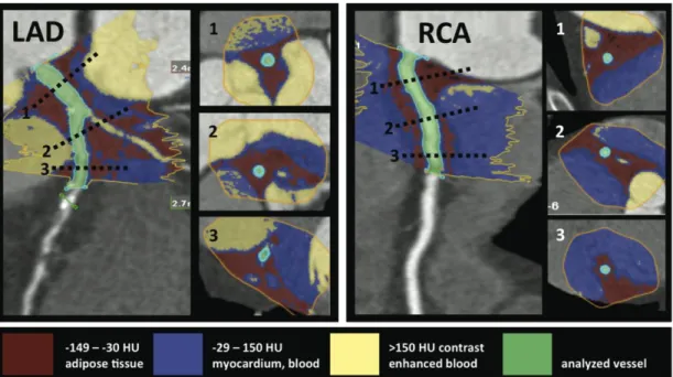
We started the PCAT quantification at the ostium of the left main (LM)/left anterior descending coronary artery (LAD), left circumflex artery (LCx), and right coronary artery (RCA). The method of threshold-based volumetric PCAT assessment is based on a modified application of software for volumetric assessment of coronary atherosclerotic plaques (Vitrea 2, Version 3.9.0.1, Vital Images Inc, Plymouth, MN and SUREPlaque, Toshiba Medical Systems, Tustin, CA). Manual tracing was used to circle the region containing PCAT in cross-sectional images perpendicular to the vessel centerline in every 5 mm. The exact pericoronary fat volume within the manually traced region was calculated by the software using Hounsfield unit (HU) based thresholds (Figure 1).
Figure 1 - Threshold based volumetric pericoronary adipose tissue quantification (left panel: LAD, right panel: RCA). The inserted cross-sections correspond to levels marked with dotted lines on the LAD and RCA. The manual tracing (yellow line) of the region of interest is performed on muliplanar-reformatted images perpendicular to the vessel centerline. The voxels within the predefined Hounsfield unit range are summarized, and the adipose tissue volume is calculated automatically. The red color indicates fat containing voxels. The blue color indicates the vessel wall, myocardium, and the non- enhanced blood pool. The yellow color indicates the contrast enhanced blood filled lumen and cavities. The green color indicates the analyzed vessel.
Voxels with values between the minimum setting of the SUREPlaque tool (-149HU) and the widely used upper threshold (-30HU) (86) were determined to represent adipose tissue, and the total PCAT volume was calculated by summing these voxels along the course of each coronary artery. We recorded PCAT volumes in 5 mm increments, and summed PCAT along the measured vessel lengths. Voxels representing air, myocardium, or contrast enhanced blood pool in the selected region were excluded by the HU cutoffs.
Two independent readers who were blinded to the coronary plaque and hs-CRP results performed the PCAT measurements. We have analyzed the proximal part of the coronary vessels since this vessel segment has a better image quality on coronary CT angiography as compared to the distal segments (87). Furthermore, this is the most relevant vessel
portion clinically, since the proximal segments contain the majority of culprit lesions in patients with acute coronary syndromes (88). Observer 1 performed measurements around the proximal 40 mm of the coronaries in all 51 patients once. For inter-observer and intra-observer reproducibility, observer 2 performed the measurements in 20 randomly selected patients, and Observer 1 repeated this process in the same 20 patients 1 month later. A total of 153 vessels and 1224 coronary artery subsegments were evaluated across the three patient groups.
3.3.3 Coronary artery plaque assessment
The coronary plaque assessment was performed by one experienced CT reader who was blinded to the PCAT volume and hs-CRP results. To determine the exact anatomic location of coronary plaques, the first 40 mm of the LM/LAD, LCx, and the RCA were evaluated using axial images, multiplanar reconstructions, thin-slab maximum intensity projections, and curved multiplanar reformatted images. The presence of coronary plaque was evaluated in 5 mm subsegments of each vessel: 0-5 mm, 5-10 mm, 10-15 mm, 15-20 mm, 20-25 mm, 25-30 mm, 30-35 mm, and 35-40 mm positions from the ostium.
3.3.4 Hs-CRP assessment
Blood samples from the peripheral vein were collected in an EDTA-coated tube within one hour prior to the coronary CT angiography scan. The samples were immediately centrifuged with the plasma aliquoted and stored at -80°C until analysis. Concentrations of hs-CRP were measured nephelometrically on a BN II analyzer (Dade-Behring, Marburg, Germany). Inter-assay coefficients of variation were <5% for nephelometry.
Hs-CRP levels were defined as high if >2.0 mg/L and low if <1.0 mg/L, as described above.
3.4 Statistical analysis
3.4.1 Abdominal fat quantification reproducibility study: Statistical considerations
Two experienced observers performed an analysis of all 100 datasets in random order to assess for inter-observer variability, blinded to the readings by the other observer. One reader repeated the analysis one week later to assess for intra-observer variability. Inter- and intra-observer reproducibility was assessed using the intra-class correlation coefficient (ICC) (89). A value close to 1 indicates excellent agreement between the two readings. In addition, the significance of the mean difference between the two readings was assessed using the paired t-test. Similar analysis was used to compare single- and volumetric- measurements for the first reading of the primary reader. The age and sex effect on the difference between single- and volumetric-subjects were assessed individually using one-way analysis of variance. A p-value < 0.05 was considered to indicate statistical significance.
3.4.2 Abdominal adipose tissue and metabolic risk factors: Statistical considerations
SAV and VAV were normally distributed. Sex-specific age-adjusted Pearson correlation coefficients were used to assess simple correlations between SAV and VAV and metabolic risk factors. Multivariable linear and logistic regression was used to assess the significance of covariate-adjusted cross-sectional relations between continuous and dichotomous metabolic risk factors and SAT and VAT. For continuous risk factors, the covariate-adjusted average change in risk factor per 1–standard deviation (SD) increase in adipose tissue was estimated; for dichotomous risk factors, the change in odds of the risk factor prevalence per 1-SD increase in adipose tissue was estimated. All models were sex specific to account for the strong sex interactions observed. Covariates in all models included age, smoking (3-level variable: current/former/never smoker), physical activity, alcohol use (dichotomized at >14 drinks per week in men or >7 drinks per week in women), menopausal status, and hormone replacement therapy. In addition, lipid treatment, hypertension treatment, and diabetes treatment were included as covariates in
models for HDL cholesterol, log triglycerides, systolic and diastolic blood pressures, and fasting plasma glucose, respectively. R2 values were computed for continuous models and c statistics were computed for dichotomous models to assess the relative contribution of SAT and VAT to explain the outcomes (risk factors). For each risk factor, tests for the significance of the difference between the SAT and VAT regression coefficients were carried out within a multivariate standardized regression (in which variables were first standardized to a mean of 0 and an SD of 1) to assess the relative importance of each adipose tissue measurement in predicting the risk factor. To assess the incremental utility of adding VAT to models that contain BMI or WL, the above multivariate analyses were repeated for VAT with BMI and WL added as covariates in the multivariate regression models. Similar models were not examined for SAT because models with SAT alone did not yield higher R2 or c statistics than models that included BMI and WL alone. As a secondary analysis, the above multivariate regressions were rerun using the general estimating equation linear and logistic regression (90) account for correlations among related individuals (siblings) in the study sample. SAS version 8.0 was used to perform all computations; a 2-tailed value of P<0.05 was considered significant (90).
3.4.3 Abdominal adipose tissue and markers of inflammation: Statistical considerations
All biomarkers were log-transformed due to their skewed distributions. Analyses described below were sex-pooled, except for CRP analyses, which were performed for each sex separately as we observed a significant sex-interaction.
Age- and sex-adjusted Pearson partial correlation coefficients were used to assess correlations between SAT and VAT and biomarkers. In our primary analysis multivariable linear regression models were constructed for each biomarker (dependent variable) versus each of SAT and VAT separately adjusted for age, sex, cigarette smoking (current, former, never smoker), chronic aspirin use, alcohol consumption, menopausal status, hormone replacement therapy, and physical activity index. R2 were computed to assess the relative contribution of SAT and VAT towards explaining the variance in each biomarker. For each marker that was significantly correlated with both SAT and VAT, we used multivariable regressions to assess the significance of the marker
relationship with SAT in the presence of VAT and vice-versa.
We report the magnitude of the association of SAT and VAT with each biomarker concentration by calculating regression coefficients quantifying the estimated change in log transformed biomarker per standard deviation increase in SAT and VAT separately, and then transforming back to original biomarker units. SAT and VAT were first standardized to a mean of 0 and standard deviation of 1. Multivariable linear regression containing both SAT and VAT as regressor variables were used to compare the SAT and VAT beta-coefficients for each marker. We then examined the residual effect size of SAT and VAT as it related to each biomarker in models containing the above-mentioned risk factors and BMI and WL. Secondarily, we examined the significance of BMI and WL in these multivariable-adjusted models containing SAT or VAT.
We performed several additional secondary analyses. First, we tested for the presence of interactions of VAT and SAT with sex, age (above/below the median age of 60 years), smoking (current, former, never), and obesity (yes/no) in the above multivariable models (without BMI and WL as independent variables). Second, we performed analyses excluding individuals with diabetes or prevalent cardiovascular disease as determined at exam seven. Third, we conducted analyses also adjusting for systolic blood pressure, diastolic blood pressure, hypertension treatment, lipid treatment, total/high density lipoprotein cholesterol ratio, triglycerides, diabetes, and prevalent cardiovascular disease.
Finally, we conducted exploratory analyses excluding individuals with CRP>10 mg/L at examination seven to account for acute inflammatory states.
To account for multiple testing, we limited our definition of statistical significance to a two-tailed p<0.05 for primary analyses (for each individual marker), and p<0.01 for all secondary analyses. SAS version 8.0 was used to perform all computations (90).
3.4.4 Pericoronary adipose tissue quantification: Statistical considerations
Continuous variables are reported as mean ± standard deviation (SD) or median and interquartile range (IQR), as appropriate. Discrete variables are given in frequency and percentiles. To compare the differences in characteristics between the three groups, we used analysis of variance (ANOVA) or Kruskal-Wallis test for continuous variables as
appropriate and Fisher‟s Exact test for categorical variables. For reproducibility of PCAT volumes, we used the intraclass correlation coefficient (ICC) for inter-observer and intra-observer agreement and paired t-test for determining the significance of the mean absolute and relative differences. In addition, inter-observer measures were assessed using the Pearson‟s correlation coefficient and a Bland-Altman graph. On a per- patient basis, the differences in PCAT volumes between the 3 groups were determined with ANOVA, and post-hoc two group comparisons were performed with Wilcoxon rank sum tests. We used generalized linear regression analysis to adjust for covariates with p- value <0.10 in univariate analyses, which included body mass index (BMI), hypertension, and hyperlipidemia. On a per-vessel basis, the differences in PCAT volumes between the 3 groups were assessed using ANOVA. On a per-subsegment basis, we compared the surrounding PCAT volume in the 1224 subsegments with plaque and no plaque using the Wilcoxon rank sum test and confirmed the results by using a mixed model with restricted maximum likelihood estimation to account for within-subject correlation. A two-tailed p- value of <0.05 was considered significant. All analyses were performed using the SAS software (Version 9.2, SAS Institute Inc) and SPSS 16.0 (Chicago, Illinois).
4 Results
4.1.1 The reproducibility study
The mean SAV was 2929.8 ± 1260.0 cm3 (range of 501.0 – 6695.0) and the mean VAV was 2031.6 ± 1013.7 cm3 (range of 288.0 – 4731.0). The mean SAA was 543.5 ± 252.4 cm2 and the mean SAA was 325.9 ± 162.3 cm2. The mean WL was 100.0 ± 12.3 cm (range of 74.9 – 131.3) and the mean SD was 24.2 ± 4.0 cm (range of 15.9 – 35.9).
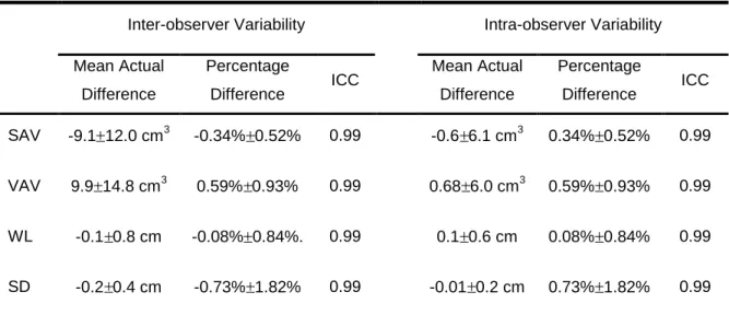
4.1.2 Intra-observer variability
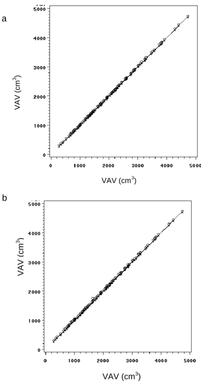
The intra-observer reproducibility was excellent for SAV and VAV (ICC=0.99; Figure 2a). The mean absolute and relative intra-observer differences were small and non- significant for both measurements (SAV: -0.6 ± 6.1 cm3, p=0.29; VAV: 0.7 ± 6.0 cm3; p=0.26).
The mean absolute difference was 0.1 ± 0.6 cm (p=0.09) for WL measurements and -0.01
± 0.2 cm (p=0.68) for SD measurements (Table 3). Both WL and SD measurements were highly correlated (ICC: 0.99).
Figure 2 - a) Intra- and b) Inter-reader correlation of volumetric measurements of abdominal adipose tissue. Absolute mean intra-observer differences: 0.68 6.0 cm3; ICC=0.99 (b) Absolute mean inter-observer differences: 9.9 14.8 cm3; ICC=0.99.
VAV (cm3 )
VAV (cm3) b
VAV (cm3)
a
VAV (cm3 )
4.1.3 Inter-observer variability
The mean absolute inter-observer differences were extremely small and both measurements were highly correlated (SAV: -9.1 ± 12.0 cm3, ICC=0.99, and VAV: 9.9 ± 14.8 cm3; ICC=0.99 (Figure 2b)). The relative difference between observers was small and non-significant -0.34% ± 0.52% for SAV and 0.59% ± 0.93% for VAV (p=n.s.).
The mean WL was 100.0 ± 12.3 cm (range of 74.9 – 131.3) with a mean absolute difference of -0.1 ± 0.8 cm and a mean relative difference of -0.08% ± 0.84% between the two observers (ICC=0.99). The mean SD was 24.2 ± 4.0 cm (range of 15.9 – 35.9) with a mean absolute difference of -0.2 ± 0.4 cm and a mean relative difference of - 0.73% ± 1.82% (ICC=0.99); (Table 3).
Table 3 - Inter- and intra-observer correlation.
Inter-observer Variability Intra-observer Variability
Mean Actual Difference
Percentage
Difference ICC Mean Actual Difference
Percentage
Difference ICC
SAV -9.1 12.0 cm3 -0.34% 0.52% 0.99 -0.6 6.1 cm3 0.34% 0.52% 0.99
VAV 9.9 14.8 cm3 0.59% 0.93% 0.99 0.68 6.0 cm3 0.59% 0.93% 0.99
WL -0.1 0.8 cm -0.08% 0.84%. 0.99 0.1 0.6 cm 0.08% 0.84% 0.99
SD -0.2 0.4 cm -0.73% 1.82% 0.99 -0.01 0.2 cm 0.73% 1.82% 0.99
Abbreviations: ICC, Intra Class Correlation; SAV, Subcutaneous Adipose Tissue Volume; VAV, Visceral Adipose Tissue Volume; WL, Waist Circumference; SD, Sagital Diameter.
4.1.4 Ratio of subcutaneous and visceral adipose tissue volumes
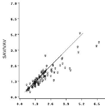
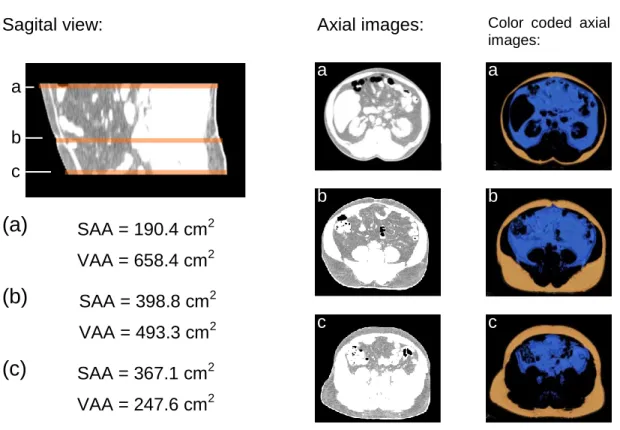
The mean SAA/VAA ratio (2.0 ± 1.2; range: 0.5 – 6.7) was significantly greater than the mean SAV/VAV ratio (1.7 ± 0.9; range: 0.4 – 5.3); (p<0.001) (Figure 3). This difference was more evident in 22 subjects with a SAA/VAA ratio ≥ 2.5 (mean difference: -0.9 ± 0.7; p<0.001). An example for the difference between planimetric and volumetric based assessment of adipose tissue distribution is given in Figure 4.
Figure 3 - Association between volume and area based measurements of the ratio between subcutaneous and visceral adipose tissue. The mean SAV/VAV ratio was significantly different from the mean SAA/VAA ratio (1.7 0.9 vs. 2.0 1.2;
respectively) with a relative difference of 11.1% (p<0.001), ICC: 0.84 SAV:
Subcutaneous adipose tissue volume, VAV: Visceral adipose tissue volume, SAA:
Subcutaneous adipose tissue area, VAA: Visceral adipose tissue area
SAA/VAA
SAV/VAV
Figure 4 - Example of the variable distribution of visceral and subcutaneous abdominal adipose tissue in a 56 year old men. Area based measurements performed at the level of the umbilicus (b); level L4/L5 (a), and S1 level (c). Ratios between subcutaneous and visceral adipose tissue vary considerably in this subject. The color coded axial images are the result of semi automatic segmentation (blue= visceral adipose tissue;
orange=subcutaneous adipose tissue).
4.1.5 Relation of volumetric based adipose tissue measurements to WL, SD, and BMI
Both SAV and VAV were highly correlated to anthropometric measurements (for SAV:
r=0.83, 0.73, 0.75 and for VAV: r=0.76, 0.85, 0.70; for WL, SD, and BMI; respectively, all p<0.0001). In contrast, the ratio of SAV to SAV was only weakly inversely associated with SD (r=-0.32, p=0.01) and not correlated with WL (r=-0.14, p=0.14) or BMI (r=- 0.17, p=0.09). As expected, anthropometric measurements were strongly correlated with each other (BMI vs. WL r=0.87, p<0.0001; BMI vs. SD r=0.84, p<0.001; and SD vs. WL r=0.94, p<0.0001).
SAA = 190.4 cm2 VAA = 658.4 cm2 SAA/VFA = 0.29
SAA = 398.8 cm2 VAA = 493.3 cm2 SAA/VFA = 0.81 SAA = 367.1 cm2 VAA = 247.6 cm2 SFA/VFA = 1.48
Sagital view: Axial images:
a
b
c
Color coded axial images:
a
b
c
(a)
(b)
(c)
a b c
4.1.6 Abdominal adipose tissue distribution by age and sex
In order to determine whether volumetric measurements reflect differences in abdominal adipose tissue distribution related to age, we stratified our population to above (n=51) and below (n=49) the mean age (59.9 ± 12.9 years). The mean SAV/VAV ratio was significantly higher in subjects <60 years of age as compared to subjects > 60 years (1.9
± 1.0 vs. 1.5 ± 0.7; p<0.001). In addition, we examined for possible differences between men and women, and we found that men had significantly lower SAV/VAV ratios than women independent of age (1.2 ± 0.5 vs. 2.2 ± 0.9 for men vs. women; respectively (p<0.001)).
4.2 The abdominal adipose tissue depots and metabolic risk factors
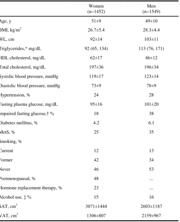
Overall, 1452 women and 1549 men were available for analysis. The mean age was 50 years (Table 4); approximately one quarter of the sample was hypertensive, 5% had diabetes, and approximately one third had MetS. Approximately half of the women were postmenopausal.
In the analysis regarding the metabolic risk factors the third generation's participants were included as well. The mean SAT volume among the offspring and the third gen participants was 3071±1444 cm3 in women and 2603±1187 cm3 in men. The mean VAT volume in women was 1306±807 cm3 and in men was 2159±967 cm3.
Table 4 - Clinical characteristics of study participants free of clinical CVD who underwent MDCT assessment of SAT and VAT volumes
Women (n=1452)
Men (n=1549)
Age, y 51±9 49±10
BMI, kg/m2 26.7±5.4 28.3±4.4
WL, cm 92±14 103±11
Triglycerides,* mg/dL 92 (65, 134) 113 (76, 171)
HDL cholesterol, mg/dL 62±17 46±12
Total cholesterol, mg/dL 197±36 196±34
Systolic blood pressure, mmHg 119±17 123±14
Diastolic blood pressure, mmHg 73±9 78±9
Hypertension, % 24 28
Fasting plasma glucose, mg/dL 95±16 101±20
Impaired fasting glucose,† % 18 38
Diabetes mellitus, % 4.2 6.1
MetS, % 25 35
Smoking, %
Current 12 13
Former 42 34
Never 46 53
Postmenopausal, % 48 ...
Hormone replacement therapy, % 23 ...
Alcohol use, ‡ % 15 16
SAT, cm3 3071±1444 2603±1187
VAT, cm3 1306±807 2159±967
Data are presented as mean±SD when appropriate.
*Median (25th, 75th percentiles).
†Fasting plasma glucose of 100 to 125 mg/dL; percentage is based on those without diabetes.
‡Defined as >14 drinks per week (men) or >7 drinks per week (women).
4.2.1 Correlations with SAT and VAT
Correlations of SAT and VAT with metabolic risk factors are shown in Table 4. SAT was positively correlated with age in women (r=0.13, P<0.001) but not men, and VAT was positively correlated with age in both sexes (r=0.36 in women and men, P<0.001). SAT and VAT were highly correlated, with an age-adjusted correlation coefficient between SAT and VAT of 0.71 (P<0.0001) in women and 0.58 (P<0.0001) in men. Both BMI and WL were strongly correlated with SAT and VAT after adjustment for age (Table 5). All risk factors were highly correlated with both SAT and VAT, except for serum total cholesterol with SAT in men and physical activity index with VAT in men.
Table 5 - Age-adjusted Pearson Correlation coefficients between metabolic risk factors and SAT and VAT volumes
Women Men
SAT VAT SAT VAT
Age 0.13† 0.36† 0.03† 0.36†
BMI 0.88† 0.75† 0.83† 0.71†
WL 0.87† 0.78† 0.88† 0.73†
Log triglycerides 0.31† 0.46† 0.18† 0.37†
HDL cholesterol –0.25† –0.35† –0.17† –0.33†
Total cholesterol 0.11† 0.15† 0.02 0.08*
Systolic blood pressure 0.26† 0.30† 0.18† 0.24†
Diastolic blood pressure 0.26† 0.28† 0.21† 0.27†
Blood glucose 0.23† 0.34† 0.12† 0.19†
Physical activity index –0.14† –0.09* –0.08* –0.03
*p<0.01; †p<0.001
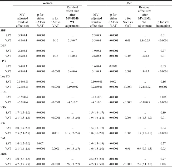
4.2.2 Multivariable-adjusted regressions with SAT, VAT, and metabolic risk factors
Results of multivariable-adjusted general linear regression analyses for SAT and VAT for both continuous and dichotomous metabolic risk factors are shown in Table 5. In women, per 1-SD increase in SAT, systolic blood pressure increased on average 3.9±0.4 mmHg (±1 SE), whereas VAT was 4.8±0.4 mmHg higher. For systolic blood pressure in women, the difference between the magnitude of effect of the SAT versus VAT was not significant (P=0.10; (Table 5.). In men, the magnitude of the association of the average systolic blood pressure increase per 1-SD increase in VAT was larger than for SAT (3.3 versus 2.3 mmHg, respectively; P=0.01 for difference in the regression coefficients between SAT and VAT). Similar results were obtained for diastolic blood pressure.
In women and men, the associations of both SAT and VAT with continuous measures of metabolic risk factors were highly significant. For fasting plasma glucose, the effect of VAT was stronger than that of SAT (P<0.0001 for difference in women, P=0.001 in men). Strong and significant results for log triglycerides and HDL cholesterol followed similar patterns (Table 6).
Highly significant associations with SAT and VAT also were noted for dichotomous risk factor variables. Among women and men, both SAT and VAT were associated with an increased odds of hypertension (Table 5). In women, the odds ratio of hypertension per 1- SD increase in VAT (odds ratio, 2.1) was stronger than that for SAT (odds ratio, 1.7;
P=0.001 for difference between SAT and VAT); similar differences were noted for men.
Similar highly significant differences also were noted for impaired fasting glucose, diabetes, and MetS and are presented in Table 5.
The magnitude of association between VAT and all risk factors examined was consistently greater for women than for men (Table 5). Weaker sex differences were observed for SAT.
Table 6 - Gender-specific multivariable-adjusted* regressions for SAT and VAT with continuous metabolic risk factors (top) and dichotomous risk factors (bottom)
Women Men
MV- adjusted residual effect size
p for either SAT or
VAT
p for SAT vs
VAT
Residual effect size
after MV/BMI/
WL adjustment
MV- adjusted residual effect size
p for either SAT or
VAT
p for SAT vs
VAT
Residual effect size
after MV/BMI/
WL adjustment
p for sex interaction SBP
SAT 3.9±0.4 <0.0001 ... 2.3±0.3 <0.0001 ... 0.01
VAT 4.8±0.4 <0.0001 0.10 2.5±0.7 3.3±0.4 <0.0001 0.01 1.8±0.05 <0.0001
DBP
SAT 2.2±0.2 <0.0001 ... 1.9±0.2 <0.0001 ... 0.77
VAT 2.6±0.3 <0.0001 0.33 1.4±0.4 2.6±0.2 <0.0001 0.008 1.5±0.3 0.01
FPG
SAT 3.4±0.3 <0.0001 ... 1.6±0.4 0.0002 ... 0.03
VAT 4.8±0.4 <0.0001 <0.0001 3.4±0.6 3.1±0.5 <0.0001 0.001 1.8±0.7 <0.0001
Log TG
SAT 0.14±0.01 <0.0001 ... 0.10±0.01 0.003 ... 0.16
VAT 0.23±0.01 <0.0001 <0.0001 0.19±0.02 0.22±0.01 <0.0001 <0.0001 0.22±0.02 0.0002 HDL
SAT –3.9±0.4 <0.0001 ... –2.0±0.3 <0.0001 ... 0.006
VAT –5.9±0.4 <0.0001 <0.0001 –4.5±0.7 –4.5±0.3 <0.0001 <0.0001 –3.8±0.5 <0.0001 HTN
SAT 1.7 (1.5–2.0) <0.0001 ... 1.5 (1.4–1.7) <0.0001 ... 0.89
VAT 2.1 (1.8–2.4) <0.0001 <0.0001 1.6 (1.3–2.0) 1.9 (1.6–2.1) <0.0001 0.006 1.6 (1.3–1.9) 0.01 IFG
SAT 2.0 (1.7–2.3) <0.0001 ... 1.5 (1.3–1.7) <0.0001 ... 0.04
VAT 2.5 (2.1–2.9) <0.0001 0.001 2.1 (1.7–2.6) 1.8 (1.6–2.0) <0.0001 0.005 1.5 (1.2–1.8) <0.0001 DM
SAT 1.6 (1.2–2.0) 0.007 ... 1.6 (1.3–1.9) <0.0001 ... 0.27
VAT 2.1 (1.6–2.6) <0.0001 0.0003 1.9 (1.3–2.7) 1.6 (1.3–2.0) <0.0001 0.91 0.9 (0.7–1.3) 0.03 MetS
SAT 3.0 (2.6–3.5) <0.0001 ... 2.5 (2.2–2.8) <0.0001 ... 0.77
VAT 4.7 (3.9–5.7) <0.0001 <0.0001 1.9 (1.3–2.7) 4.2 (3.5–5.0) <0.0001 <0.0001 2.6 (2.1–3.2) 0.002 MV indicates multivariable; SBP, systolic blood pressure; DBP, diastolic blood pressure; FPG, fasting plasma glucose; TG, triglycerides; HTN, hypertension; IFG, impaired fasting glucose; and DM, diastolic mellitus. Data presented include effect size (the average change in risk factor�SE) per 1 SD in adipose tissue for continuous data, and the change in odds of the condition per 1 SD of adipose tissue with 95% CIs for dichotomous data.
*Adjusted for age, smoking, alcohol use, physical activity, and menopausal status (women only), hormone replacement therapy (women only); for blood pressure, FPG, HDL cholesterol, and log triglycerides, an additional covariate of treatment for HTN, diabetes, or lipid disorders, respectively, was included.
†For SAT or VAT in the model. ‡For SAT vs VAT difference.