Astronomy &
Astrophysics Special issue
https://doi.org/10.1051/0004-6361/201832843
© ESO 2018
Gaia Data Release 2
Gaia Data Release 2
Observational Hertzsprung-Russell diagrams ?
Gaia Collaboration, C. Babusiaux
1,2,??, F. van Leeuwen
3, M. A. Barstow
4, C. Jordi
5, A. Vallenari
6, D. Bossini
6, A. Bressan
7, T. Cantat-Gaudin
6,5, M. van Leeuwen
3, A. G. A. Brown
8, T. Prusti
9, J. H. J. de Bruijne
9, C. A. L. Bailer-Jones
10, M. Biermann
11, D. W. Evans
3, L. Eyer
12, F. Jansen
13, S. A. Klioner
14, U. Lammers
15, L. Lindegren
16, X. Luri
5, F. Mignard
17, C. Panem
18, D. Pourbaix
19,20, S. Randich
21, P. Sartoretti
2, H. I. Siddiqui
22,
C. Soubiran
23, N. A. Walton
3, F. Arenou
2, U. Bastian
11, M. Cropper
24, R. Drimmel
25, D. Katz
2, M. G. Lattanzi
25, J. Bakker
15, C. Cacciari
26, J. Castañeda
5, L. Chaoul
18, N. Cheek
27, F. De Angeli
3, C. Fabricius
5, R. Guerra
15, B. Holl
12, E. Masana
5, R. Messineo
28, N. Mowlavi
12, K. Nienartowicz
29, P. Panuzzo
2, J. Portell
5, M. Riello
3, G. M. Seabroke
24, P. Tanga
17, F. Thévenin
17, G. Gracia-Abril
30,11, G. Comoretto
22, M. Garcia-Reinaldos
15,
D. Teyssier
22, M. Altmann
11,31, R. Andrae
10, M. Audard
12, I. Bellas-Velidis
32, K. Benson
24, J. Berthier
33, R. Blomme
34, P. Burgess
3, G. Busso
3, B. Carry
17,33, A. Cellino
25, G. Clementini
26, M. Clotet
5, O. Creevey
17,
M. Davidson
35, J. De Ridder
36, L. Delchambre
37, A. Dell’Oro
21, C. Ducourant
23, J. Fernández-Hernández
38, M. Fouesneau
10, Y. Frémat
34, L. Galluccio
17, M. García-Torres
39, J. González-Núñez
27,40, J. J. González-Vidal
5,
E. Gosset
37,20, L. P. Guy
29,41, J.-L. Halbwachs
42, N. C. Hambly
35, D. L. Harrison
3,43, J. Hernández
15, D. Hestroffer
33, S. T. Hodgkin
3, A. Hutton
44, G. Jasniewicz
45, A. Jean-Antoine-Piccolo
18, S. Jordan
11, A. J. Korn
46, A. Krone-Martins
47, A. C. Lanzafame
48,49, T. Lebzelter
50, W. Löffler
11, M. Manteiga
51,52,
P. M. Marrese
53,54, J. M. Martín-Fleitas
44, A. Moitinho
47, A. Mora
44, K. Muinonen
55,56, J. Osinde
57, E. Pancino
21,54, T. Pauwels
34, J.-M. Petit
58, A. Recio-Blanco
17, P. J. Richards
59, L. Rimoldini
29, A. C. Robin
58,
L. M. Sarro
60, C. Siopis
19, M. Smith
24, A. Sozzetti
25, M. Süveges
10, J. Torra
5, W. van Reeven
44, U. Abbas
25, A. Abreu Aramburu
61, S. Accart
62, C. Aerts
36,63, G. Altavilla
53,54,26, M. A. Álvarez
51, R. Alvarez
15, J. Alves
50,
R. I. Anderson
64,12, A. H. Andrei
65,66,31, E. Anglada Varela
38, E. Antiche
5, T. Antoja
9,5, B. Arcay
51, T. L. Astraatmadja
10,67, N. Bach
44, S. G. Baker
24, L. Balaguer-Núñez
5, P. Balm
22, C. Barache
31, C. Barata
47,
D. Barbato
68,25, F. Barblan
12, P. S. Barklem
46, D. Barrado
69, M. Barros
47, S. Bartholomé Muñoz
5,
J.-L. Bassilana
62, U. Becciani
49, M. Bellazzini
26, A. Berihuete
70, S. Bertone
25,31,71, L. Bianchi
72, O. Bienaymé
42, S. Blanco-Cuaresma
12,23,73, T. Boch
42, C. Boeche
6, A. Bombrun
74, R. Borrachero
5, S. Bouquillon
31, G. Bourda
23,
A. Bragaglia
26, L. Bramante
28, M. A. Breddels
75, N. Brouillet
23, T. Brüsemeister
11, E. Brugaletta
49, B. Bucciarelli
25, A. Burlacu
18, D. Busonero
25, A. G. Butkevich
14, R. Buzzi
25, E. Caffau
2, R. Cancelliere
76,
G. Cannizzaro
77,63, R. Carballo
78, T. Carlucci
31, J. M. Carrasco
5, L. Casamiquela
5, M. Castellani
53, A. Castro-Ginard
5, P. Charlot
23, L. Chemin
79, A. Chiavassa
17, G. Cocozza
26, G. Costigan
8, S. Cowell
3, F. Crifo
2,
M. Crosta
25, C. Crowley
74, J. Cuypers
†34, C. Dafonte
51, Y. Damerdji
37,80, A. Dapergolas
32, P. David
33, M. David
81, P. de Laverny
17, F. De Luise
82, R. De March
28, D. de Martino
83, R. de Souza
84, A. de Torres
74,
J. Debosscher
36, E. del Pozo
44, M. Delbo
17, A. Delgado
3, H. E. Delgado
60, S. Diakite
58, C. Diener
3, E. Distefano
49, C. Dolding
24, P. Drazinos
85, J. Durán
57, B. Edvardsson
46, H. Enke
86, K. Eriksson
46, P. Esquej
87, G. Eynard Bontemps
18, C. Fabre
88, M. Fabrizio
53,54, S. Faigler
89, A. J. Falcão
90, M. Farràs Casas
5, L. Federici
26,
G. Fedorets
55, P. Fernique
42, F. Figueras
5, F. Filippi
28, K. Findeisen
2, A. Fonti
28, E. Fraile
87, M. Fraser
3,91, B. Frézouls
18, M. Gai
25, S. Galleti
26, D. Garabato
51, F. García-Sedano
60, A. Garofalo
92,26, N. Garralda
5, A. Gavel
46, P. Gavras
2,32,85, J. Gerssen
86, R. Geyer
14, P. Giacobbe
25, G. Gilmore
3, S. Girona
93, G. Giuffrida
54,53,
F. Glass
12, M. Gomes
47, M. Granvik
55,94, A. Gueguen
2,95, A. Guerrier
62, J. Guiraud
18, R. Gutiérrez-Sánchez
22, R. Haigron
2, D. Hatzidimitriou
85,32, M. Hauser
11,10, M. Haywood
2, U. Heiter
46, A. Helmi
75, J. Heu
2, T. Hilger
14,
D. Hobbs
16, W. Hofmann
11, G. Holland
3, H. E. Huckle
24, A. Hypki
8,96, V. Icardi
28, K. Janßen
86, G. Jevardat de Fombelle
29, P. G. Jonker
77,63, Á. L. Juhász
97,98, F. Julbe
5, A. Karampelas
85,99, A. Kewley
3,
?The full Table A.1 is only available at the CDS via anonymous ftp to cdsarc.u-strasbg.fr (130.79.128.5) or via http://cdsarc.u-strasbg.fr/viz-bin/qcat?J/A+A/616/A10
??Corresponding author: C. Babusiaux, e-mail:carine.babusiaux@univ-grenoble-alpes.fr
A10, page 1 of29
Open Access article,published by EDP Sciences, under the terms of the Creative Commons Attribution License (http://creativecommons.org/licenses/by/4.0),
J. Klar
86, A. Kochoska
100,101, R. Kohley
15, K. Kolenberg
73,102,36, M. Kontizas
85, E. Kontizas
32, S. E. Koposov
3,103, G. Kordopatis
17, Z. Kostrzewa-Rutkowska
77,63, P. Koubsky
104, S. Lambert
31, A. F. Lanza
49, Y. Lasne
62,
J.-B. Lavigne
62, Y. Le Fustec
105, C. Le Poncin-Lafitte
31, Y. Lebreton
2,106, S. Leccia
83, N. Leclerc
2, I. Lecoeur-Taibi
29, H. Lenhardt
11, F. Leroux
62, S. Liao
25,107,108, E. Licata
72, H. E. P. Lindstrøm
109,110, T. A. Lister
111, E. Livanou
85, A. Lobel
34, M. López
69, S. Managau
62, R. G. Mann
35, G. Mantelet
11, O. Marchal
2,
J. M. Marchant
112, M. Marconi
83, S. Marinoni
53,54, G. Marschalkó
97,113, D. J. Marshall
114, M. Martino
28, G. Marton
97, N. Mary
62, D. Massari
75, G. Matijeviˇc
86, T. Mazeh
89, P. J. McMillan
16, S. Messina
49, D. Michalik
16,
N. R. Millar
3, D. Molina
5, R. Molinaro
83, L. Molnár
97, P. Montegriffo
26, R. Mor
5, R. Morbidelli
25, T. Morel
37, D. Morris
35, A. F. Mulone
28, T. Muraveva
26, I. Musella
83, G. Nelemans
63,36, L. Nicastro
26, L. Noval
62, W. O’Mullane
15,41, C. Ordénovic
17, D. Ordóñez-Blanco
29, P. Osborne
3, C. Pagani
4, I. Pagano
49, F. Pailler
18, H. Palacin
62, L. Palaversa
3,12, A. Panahi
89, M. Pawlak
115,116, A. M. Piersimoni
82, F.-X. Pineau
42, E. Plachy
97, G. Plum
2, E. Poggio
68,25, E. Poujoulet
117, A. Prša
101, L. Pulone
53, E. Racero
27, S. Ragaini
26, N. Rambaux
33,
M. Ramos-Lerate
118, S. Regibo
36, C. Reylé
58, F. Riclet
18, V. Ripepi
83, A. Riva
25, A. Rivard
62, G. Rixon
3, T. Roegiers
119, M. Roelens
12, M. Romero-Gómez
5, N. Rowell
35, F. Royer
2, L. Ruiz-Dern
2, G. Sadowski
19, T. Sagristà Sellés
11, J. Sahlmann
15,120, J. Salgado
121, E. Salguero
38, N. Sanna
21, T. Santana-Ros
96, M. Sarasso
25,
H. Savietto
122, M. Schultheis
17, E. Sciacca
49, M. Segol
123, J. C. Segovia
27, D. Ségransan
12, I-C. Shih
2, L. Siltala
55,124, A. F. Silva
47, R. L. Smart
25, K. W. Smith
10, E. Solano
69,125, F. Solitro
28, R. Sordo
6, S. Soria Nieto
5, J. Souchay
31, A. Spagna
25, F. Spoto
17,33, U. Stampa
11, I. A. Steele
112, H. Steidelmüller
14, C. A. Stephenson
22, H. Stoev
126, F. F. Suess
3, J. Surdej
37, L. Szabados
97, E. Szegedi-Elek
97, D. Tapiador
127,128, F. Taris
31, G. Tauran
62, M. B. Taylor
129, R. Teixeira
84, D. Terrett
59, P. Teyssandier
31, W. Thuillot
33, A. Titarenko
17,
F. Torra Clotet
130, C. Turon
2, A. Ulla
131, E. Utrilla
44, S. Uzzi
28, M. Vaillant
62, G. Valentini
82, V. Valette
18, A. van Elteren
8, E. Van Hemelryck
34, M. Vaschetto
28, A. Vecchiato
25, J. Veljanoski
75, Y. Viala
2, D. Vicente
93, S. Vogt
119, C. von Essen
132, H. Voss
5, V. Votruba
104, S. Voutsinas
35, G. Walmsley
18, M. Weiler
5, O. Wertz
133, T. Wevers
3,63, Ł. Wyrzykowski
3,115, A. Yoldas
3, M. Žerjal
100,134, H. Ziaeepour
58, J. Zorec
135, S. Zschocke
14,
S. Zucker
136, C. Zurbach
45, and T. Zwitter
100(Affiliations can be found after the references)
Received 16 February 2018 / Accepted 16 April 2018
ABSTRACT
Context. Gaia Data Release 2 provides high-precision astrometry and three-band photometry for about 1.3 billion sources over the full sky. The precision, accuracy, and homogeneity of both astrometry and photometry are unprecedented.
Aims. We highlight the power of theGaiaDR2 in studying many fine structures of the Hertzsprung-Russell diagram (HRD).Gaia allows us to present many different HRDs, depending in particular on stellar population selections. We do not aim here for completeness in terms of types of stars or stellar evolutionary aspects. Instead, we have chosen several illustrative examples.
Methods. We describe some of the selections that can be made inGaiaDR2 to highlight the main structures of theGaiaHRDs.
We select both field and cluster (open and globular) stars, compare the observations with previous classifications and with stellar evolutionary tracks, and we present variations of theGaiaHRD with age, metallicity, and kinematics. Late stages of stellar evolution such as hot subdwarfs, post-AGB stars, planetary nebulae, and white dwarfs are also analysed, as well as low-mass brown dwarf objects.
Results. TheGaiaHRDs are unprecedented in both precision and coverage of the various Milky Way stellar populations and stellar evolutionary phases. Many fine structures of the HRDs are presented. The clear split of the white dwarf sequence into hydrogen and helium white dwarfs is presented for the first time in an HRD. The relation between kinematics and the HRD is nicely illustrated.
Two different populations in a classical kinematic selection of the halo are unambiguously identified in the HRD. Membership and mean parameters for a selected list of open clusters are provided. They allow drawing very detailed cluster sequences, highlighting fine structures, and providing extremely precise empirical isochrones that will lead to more insight in stellar physics.
Conclusions. GaiaDR2 demonstrates the potential of combining precise astrometry and photometry for large samples for studies in stellar evolution and stellar population and opens an entire new area for HRD-based studies.
Key words. parallaxes – Hertzsprung-Russell and C-M diagrams – solar neighborhood – stars: evolution 1. Introduction
The Hertzsprung-Russell diagram (HRD) is one of the most important tools in stellar studies. It illustrates empirically the relationship between stellar spectral type (or temperature or colour index) and luminosity (or absolute magnitude). The position of a star in the HRD is mainly given by its initial mass, chemical composition, and age, but effects such as rotation,
stellar wind, magnetic field, detailed chemical abundance, over- shooting, and non-local thermal equilibrium also play a role.
Therefore, the detailed HRD features are important to constrain stellar structure and evolutionary studies as well as stellar atmo- sphere modelling. Up to now, a proper understanding of the physical process in the stellar interior and the exact contribution of each of the effects mentioned are missing because we lack large precise and homogeneous samples that cover the full
HRD. Moreover, a precise HRD provides a great framework for exploring stellar populations and stellar systems.
Up to now, the most complete solar neighbourhood empiri- cal HRD could be obtained by combining the HIPPARCOSdata (Perryman et al. 1995) with nearby stellar catalogues to provide the faint end (e.g. Gliese & Jahreiß 1991; Henry & Jao 2015).
Clusters provide empirical HRDs for a range of ages and metal contents and are therefore widely used in stellar evolution stud- ies. To be conclusive, they need homogeneous photometry for inter-comparisons and astrometry for good memberships.
With its global census of the whole sky, homogeneous astrometry, and photometry of unprecedented accuracy, Gaia DR2 is setting a new major step in stellar, galactic, and extra- galactic studies. It provides position, trigonometric parallax, and proper motion as well as three broad-band magnitudes (G,GBP, andGRP) for more than a billion objects brighter thanG∼20, plus radial velocity for sources brighter thanGRVS∼12 mag and photometry for variable stars (Gaia Collaboration 2018a). The amount, exquisite quality, and homogeneity of the data allows reaching a level of detail in the HRDs that has never been reached before. The number of open clusters with accurate parallax infor- mation is unprecedented, and new open clusters or associations will be discovered. Gaia DR2 provides absolute parallax for faint red dwarfs and the faintest white dwarfs for the first time.
This paper is one of the papers accompanying the Gaia DR2 release. The following papers describe the data used here:
Gaia Collaboration (2018a) for an overview, Lindegren et al.
(2018) for the astrometry,Evans et al.(2018) for the photometry, andArenou et al.(2018) for the global validation. Someone inter- ested in this HRD paper may also be interested in the variability in the HRD described inGaia Collaboration(2018b), in the first attempt to derive an HRD using temperatures and luminosities from theGaiaDR2 data ofAndrae et al.(2018), in the kinematics of the globular clusters discussed inGaia Collaboration(2018c), and in the field kinematics presented in Gaia Collaboration (2018d).
In this paper, Sect.2presents a global description of how we built the GaiaHRDs of both field and cluster stars, the filters that we applied, and the handling of the extinction. In Sect.3we present our selection of cluster data; the handling of the globular clusters is detailed in Gaia Collaboration(2018c) and the han- dling of the open clusters is detailed in AppendixA. Section4 discusses the main structures of theGaiaDR2 HRD. The level of the details of the white dwarf sequence is so new that it leads to a more intense discussion, which we present in a separate Sect.5.
In Sect.6we compare clusters with a set of isochrones. In Sect.7 we study the variation of theGaiaHRDs with kinematics. We finally conclude in Sect.8.
2. Building theGaiaHRDs
This paper presents the power of theGaiaDR2 astrometry and photometry in studying fine structures of the HRD. For this, we selected the most precise data, without trying to reach complete- ness. In practice, this means selecting the most precise parallax and photometry, but also handling the extinction rigorously. This can no longer be neglected with the depth of the Gaiaprecise data in this release.
2.1. Data filtering
The Gaia DR2 is unprecedented in both the quality and the quantity of its astrometric and photometric data. Still, this is an intermediate data release without a full implementation of the
complexity of the processing for an optimal usage of the data.
A detailed description of the astrometric and photometric fea- tures is given inLindegren et al.(2018) andEvans et al.(2018), respectively, andArenou et al.(2018) provides a global valida- tion of them. Here we highlight the features that are important to be taken into account in buildingGaiaDR2 HRDs and present the filters we applied in this paper.
Concerning the astrometric content (Lindegren et al. 2018), the median uncertainty for the bright source (G<14 mag) par- allax is 0.03 mas. The systematics are lower than 0.1 mas, and the parallax zeropoint error is about 0.03 mas. Significant corre- lations at small spatial scale between the astrometric parameters are also observed. Concerning the photometric content (Evans et al. 2018), the precision atG= 12 is around 1 mmag in the three passbands, with systematics at the level of 10 mmag.
Lindegren et al.(2018) described that a five-parameter solu- tion is accepted only if at least six visibility periods are used (e.g. the number of groups of observations separated from other groups by a gap of at least four days, the parameter is named
visibility_periods_usedin theGaiaarchive). The observations need to be well spread out in time to provide reliable five- parameter solutions. Here we applied a stronger filter on this parameter:visibility_periods_used>8. This removes strong out- liers, in particular at the faint end of the local HRD (Arenou et al. 2018). It also leads to more incompleteness, but this is not an issue for this paper.
The astrometric excess noise is the extra noise that must be postulated to explain the scatter of residuals in the astro- metric solution. When it is high, it either means that the astrometric solution has failed and/or that the studied object is in a multiple system for which the single-star solution is not reliable. Without filtering on the astrometric excess noise, artefacts are present in particular between the white dwarf and the main sequence in the Gaia HRDs. Some of those stars are genuine binaries, but the majority are artefacts (Arenou et al. 2018). To still see the imprint of genuine binaries on the HRD while removing most of the artefacts, we adopted the filter proposed in Appendix C of Lindegren et al.(2018):
pχ2/(ν0−5) <1.2 max(1,exp(−0.2(G−19.5)) withχ2 andν0 given as astrometric_chi2_al and astrometric_n_good_obs_al,
respectively, in theGaiaarchive. A similar clean-up of the HRD is obtained by theastrometric_excess_noise<1criterion, but this is less optimised for the bright stars because of the degrees of freedom (DOF) issue (Lindegren et al. 2018, Appendix A).
We built theGaiaHRDs by simply estimating the absolute Gaiamagnitude in theGband for individual stars using MG= G+5+5 log10($/1000), with$the parallax in milliarcseconds (plus the extinction, see next section). This is valid only when the relative precision on the parallax is lower than about 20%
(Luri et al. 2018). We aim here to examine the fine structures in the HRD revealed byGaia and therefore adopt a 10% relative precision criterion, which corresponds to an uncertainty onMG
smaller than 0.22 mag:parallax_over_error>10.
Similarly, we apply filters on the relative flux error on the G,GBP, and GRP photometry: phot_g_mean_flux_over_error>50
(σG < 0.022 mag), phot_rp_mean_flux_over_error>20, and
phot_bp_mean_flux_over_error>20 (σGXP < 0.054 mag). These criteria may remove variable stars, which are specifically studied inGaia Collaboration(2018b).
The processing of the photometric data in DR2 has not treated blends in the windows of the blue and red photometers (BP and RP). As a consequence, the measured BP and RP fluxes may include the contribution of flux from nearby sources, the highest impact being in sky areas of high stellar density, such as
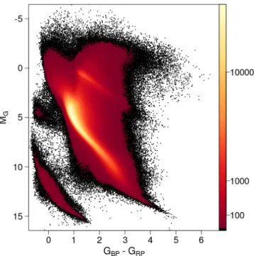
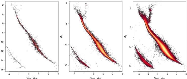
Fig. 1. FullGaia colour-magnitude diagram of sources with the fil- ters described in Sect.2.1applied (65 921 112 stars). The colour scale represents the square root of the relative density of stars.
the inner regions of globular clusters, the Magellanic Clouds, or the Galactic Bulge. During the validation process, misdetermina- tions of the local background have also been identified. In some cases, this background is due to nearby bright sources with long wings of the point spread function that have not been properly subtracted. In other cases, the background has a solar type spec- trum, which indicates that the modelling of the background flux is not good enough. The faint sources are most strongly affected.
For details, seeEvans et al.(2018) andArenou et al.(2018). Here, we have limited our analysis to the sources within the empiri- cally defined locus of the (IBP+IRP)/IGfluxes ratio as a function ofGBP−GRPcolour:phot_bp_rp_excess_factor>1.0+0.015 (GBP− GRP)2 andphot_bp_rp_excess_factor<1.3+0.06 (GBP−GRP)2. The Gaia archive query combining all the filters presented here is provided in AppendixB.
2.2. Extinction
The dust that is present along the line of sight towards the stars leads to a dimming and reddening of their observed light. In the full colour – absolute magnitude diagram presented in Fig.1, the effect of the extinction is particularly striking for the red clump.
The de-reddened HRD using the extinction provided together with DR2 is presented inAndrae et al.(2018). To study the fine structures of theGaiaHRD for field stars, we selected here only low-extinction stars. High galactic latitude and close-by stars located within the local bubble (the reddening is almost negligi- ble within∼60 pc of the SunLallement et al. 2003) are affected less from the extinction, and we did not apply further selection for them. To select low-extinction stars away from these sim- ple cases, we followedRuiz-Dern et al.(2018) and used the 3D extinction map ofCapitanio et al.(2017)1, which is particularly well adapted to finding holes in the interstellar medium and to select field stars withE(B−V)<0.015.
1 http://stilism.obspm.fr/
For globular clusters we used literature extinction values (Sect.3.3), while for open clusters, they are derived together with the ages (Sect.3.2). Detailed comparisons of these global cluster extinctions with those that can be derived from the extinctions provided by Gaia DR2 can be found inArenou et al. (2018).
To transform the global cluster extinction easily into the Gaia passbands while taking into account the extinction coefficients dependency on colour and extinction itself in these large pass- bands (e.g. Jordi et al. 2010), we used the same formulae as Danielski et al. (2018) to compute the extinction coefficients kX =AX/A0:
kX =c1+c2(GBP−GRP)0+c3(GBP−GRP)20+c4(GBP−GRP)30 +c5A0+c6A20+c7(GBP−GRP)0A0. (1) As inDanielski et al.(2018), this formula was fitted on a grid of extinctions convolving the latest Gaia passbands presented inEvans et al.(2018) with Kurucz spectra (Castelli & Kurucz 2003) and the Fitzpatrick & Massa (2007) extinction law for 3500 K<Teff <10 000 K by steps of 250 K, 0.01<A0<5 mag by steps of 0.01 mag and two surfaces gravities: logg=2.5 and 4. The resulting coefficients are provided in Table1. We assume in the followingA0=3.1E(B−V).
Some clusters show high differential extinction across their field, which broadens their colour-magnitude diagrams. These clusters have been discarded from this analysis.
3. Cluster data
Star clusters can provide observational isochrones for a range of ages and chemical compositions. Most suitable are clusters with low and uniform reddening values and whose magnitude range is wide, which would limit our sample to the nearest clusters. Such a sample would, however, present a rather limited range in age and chemical composition.
3.1. Membership and astrometric solutions
Two types of astrometric solutions were applied. The first type is applicable to nearby clusters. For the secondGaiadata release, the nearby “limit” was set at 250 pc. Within this limit, the par- allax and proper motion data for the individual cluster members are sufficiently accurate to reflect the effects of projection along the line of sight, thus enabling the 3D reconstruction of the cluster. This is further described in AppendixA.1.
For these nearby clusters, the size of the cluster relative to its distance will contribute a significant level of scatter to the HRD if parallaxes for individual cluster members are not taken into account. With a relative accuracy of about 1% in the par- allax measurement, an error contribution of around 0.02 in the absolute magnitude is possible. For a large portion of theGaia photometry, the uncertainties are about 5–10 times lower, mak- ing the parallax measurement still the main contributor to the uncertainty in the absolute magnitude. The range of differences in parallax between the cluster centre and an individual clus- ter member depends on the ratio of the cluster radius over the cluster distance. At a radius of 15 pc, the 1% level is found for a cluster at 1.5 kpc, or a parallax of 0.67 mas. In Gaia DR2, formal uncertainties on the parallaxes may reach levels of just lower than 10µas, but the overall uncertainty from localised sys- tematics is about 0.025 mas. If this value is considered the 1%
uncertainty level, then a resolution of a cluster along the line of sight, usingGaiaDR2, becomes possible for clusters within 400 pc, and realistic for clusters within about 250 pc.
Table 1.Parameters used to derive theGaiaextinction coefficients as a function of colour and extinction (Eq. (1)).
c1 c2 c3 c4 c5 c6 c7
kG 0.9761 −0.1704 0.0086 0.0011 −0.0438 0.0013 0.0099 kBP 1.1517 −0.0871 −0.0333 0.0173 −0.0230 0.0006 0.0043 kRP 0.6104 −0.0170 −0.0026 −0.0017 −0.0078 0.00005 0.0006
For clusters at larger distances, the mean cluster proper motion and parallax are derived directly from the observed astrometric parameters for the individual cluster members. The details of this procedure are presented in AppendixA.2.
3.2. Selection of open clusters
Our sample of open clusters consists of the mostly well-defined and fairly rich clusters within 250 pc, and a selection of mainly rich clusters at larger distances, covering a wider range of ages, mostly up to 1.5 kpc, with a few additional clusters at larger dis- tances where these might supply additional information at more extreme ages. For very young clusters, the definition of the clus- ter is not always clear, as the youngest systems are mostly found embedded in OB associations, producing large samples of simi- lar proper motions and parallaxes. Very few clusters appear to survive to an “old age”, but those that do are generally rich, allowing good membership determination. The final selection consists of 9 clusters within 250 pc, and 37 clusters up to 5.3 kpc.
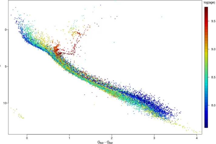
Of the latter group, only 23 were finally used for construction of the colour-magnitude diagram; these clusters are listed together with the 9 nearby clusters in Table 2. For the remaining 14 clus- ters, the colour-magnitude diagrams appeared to be too much affected by interstellar reddening variations. More details on the astrometric solutions are provided in AppendixA; the solutions are presented for the nearby clusters in Table A.3and for the more distant clusters in TableA.4. Figure2shows the combined HRD of these clusters, coloured according to their ages as pro- vided in Table 2. The main-sequence turn-off and red clump evolution with age is clearly visible. The age difference is also shown for lower mass stars, the youngest stars lie slightly above the main sequence of the others. The white dwarf sequence is also visible.
3.3. Selection of globular clusters
The details of selecting globular clusters are presented in Gaia Collaboration(2018c). A major issue for the globular clus- ter data is the uncertainties on the parallaxes that result from the systematics, which is in most cases about one order of magnitude larger than the standard uncertainties on the mean parallax deter- minations for the globular clusters. The implication of this is that the parallaxes as determined with theGaiadata cannot be used to derive the distance moduli needed to prepare the composite HRD for the globular clusters. Instead, we had to rely on distances as quoted in the literature, for which we used the tables (2010 edi- tion) provided online byHarris(1996). The inevitable drawback is that these distances and reddening values have been obtained through isochrone fitting, and the application of these values to the Gaia data will provide only limited new information. The main advantage is the possibility of comparing the HRDs of all globular clusters within a single, accurate photometric system.
The combined HRD for 14 globular clusters is shown in Fig.3, the summary data for these clusters is presented in Table3. The photometric data originate predominantly from the outskirts of
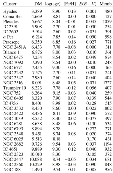
Table 2.Overview of reference values used in constructing the compos- ite HRD for open clusters (Fig.2).
Cluster DM log(age) [Fe/H] E(B−V) Memb
Hyades 3.389 8.90 0.13 0.001 480
Coma Ber 4.669 8.81 0.00 0.000 127
Pleiades 5.667 8.04 −0.01 0.045 1059
IC 2391 5.908 7.70 −0.01 0.030 254
IC 2602 5.914 7.60 −0.02 0.031 391
αPer 6.214 7.85 0.14 0.090 598
Praesepe 6.350 8.85 0.16 0.027 771
NGC 2451A 6.433 7.78 −0.08 0.000 311
Blanco 1 6.876 8.06 0.03 0.010 361
NGC 6475 7.234 8.54 0.02 0.049 874
NGC 7092 7.390 8.54 0.00 0.010 248
NGC 6774 7.455 9.30 0.16 0.080 165
NGC 2232 7.575 7.70 0.11 0.031 241
NGC 2547 7.980 7.60 −0.14 0.040 404
NGC 2516 8.091 8.48 0.05 0.071 1727
Trumpler 10 8.223 7.78 −0.12 0.056 407
NGC 752 8.264 9.15 −0.03 0.040 259
NGC 6405 8.320 7.90 0.07 0.139 544
IC 4756 8.401 8.98 0.02 0.128 515
NGC 3532 8.430 8.60 0.00 0.022 1802
NGC 2422 8.436 8.11 0.09 0.090 572
NGC 1039 8.552 8.40 0.02 0.077 497
NGC 6281 8.638 8.48 0.06 0.130 534
NGC 6793 8.894 8.78 0.272 271
NGC 2548 9.451 8.74 0.08 0.020 374
NGC 6025 9.513 8.18 0.170 431
NGC 2682 9.726 9.54 0.03 0.037 1194
IC 4651 9.889 9.30 0.12 0.040 932
NGC 2323 10.010 8.30 0.105 372
NGC 2447 10.088 8.74 −0.05 0.034 681
NGC 2360 10.229 8.98 −0.03 0.090 848
NGC 188 11.490 9.74 0.11 0.085 956
Notes. Distance moduli (DM) as derived from the Gaia astrome- try; ages and reddening values as derived fromGaiaphotometry (see Sect.6), with distances fixed on astrometric determinations; metallic- ities fromNetopil et al.(2016); Memb: the number of members with Gaiaphotometric data after application of the photometric filters.
the clusters, as in the cluster centres the crowding often affects the colour index determination. Figure3shows the blue horizon- tal branch populated with the metal-poor clusters and the move of the giant branch towards the blue with decreasing metallicity.
An interesting comparison can be made between the most metal-rich well-populated globular cluster of our sam- ple, 47 Tuc (NGC 104), and one of the oldest open clusters, M67 (NGC 2682) (Fig.4). This provides the closest compari- son between the HRDs of an open and a globular cluster. Most open clusters are much younger, while most globular clusters are much less metal rich.
Fig. 2.Composite HRD for 32 open clusters, coloured according to log(age), using the extinction and distance moduli as determined from the Gaiadata (Table2).
Fig. 3.Composite HRD for 14 globular clusters, coloured according to metallicity (Table3).
Table 3.Reference data for 14 globular clusters used in the construction of the combined HRD (Fig.3).
NGC DM Age [Fe/H] E(B−V) Memb
(Gyr)
104 13.266 12.75a −0.72 0.04 21580 288 14.747 12.50a −1.31 0.03 1953 362 14.672 11.50a −1.26 0.05 1737
1851 15.414 13.30c −1.18 0.02 744
5272 15.043 12.60b −1.50 0.01 9086 5904 14.375 12.25a −1.29 0.03 3476 6205 14.256 13.00a −1.53 0.02 10311 6218 13.406 13.25a −1.37 0.19 3127 6341 14.595 13.25a −2.31 0.02 1432 6397 11.920 13.50a −2.02 0.18 10055 6656 12.526 12.86c −1.70 0.35 9542 6752 13.010 12.50a −1.54 0.04 10779 6809 13.662 13.50a −1.94 0.08 8073 7099 14.542 13.25a −2.27 0.03 1016 Notes.Data on distance moduli (DM), [Fe/H] andE(B–V) fromHarris (1996), 2010 edition,(a)Dotter et al.(2010),(b)Denissenkov et al.(2017),
(c)Powalka et al.(2017) for age estimates. Memb: cluster members with photometry after application of photometric filters.
Fig. 4. Comparison between the HRDs of 47 Tuc (NGC 104, Age = 12.75 Gyr, [Fe/H] =−0.72), one of the most metal-rich globu- lar clusters (magenta dots), and M 67 (NGC 2682, Age = 3.47 Gyr, [Fe/H] = 0.03), one of the oldest open clusters (blue dots).
4. Details of theGaiaHRDs
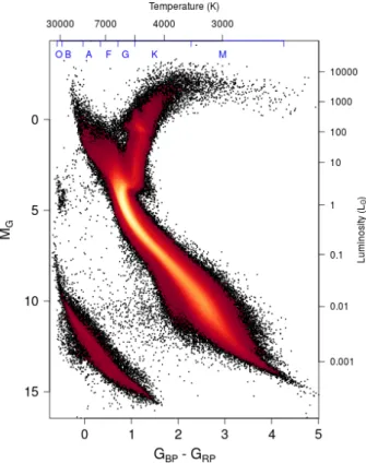
In the following, several field star HRDs are presented. Unless otherwise stated, the filters presented in Sect. 2.1, including the E(B−V) < 0.015 mag criteria, were applied. The HRDs use a red colour scale that represents the square root of the density of stars. TheGaiaDR2 HRD of the low-extinction stars is represented in Fig.5. The approximate equivalent temperature and luminosity to theGBP−GRP colour and the absoluteGaia MG magnitude provided in the figure were determined using the PARSEC isochrones (Marigo et al. 2017) for main-sequence stars.
Figure6shows the localGaia HRDs using several cuts in parallax, still with the filters of Sect.2.1, but without the need to apply theE(B−V)<0.015 mag extinction criteria, as these sources mostly lie within the local bubble.
4.1. Main sequence
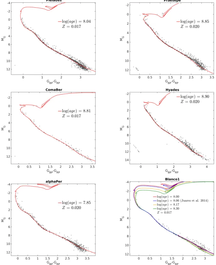
The main sequence is very thin, both in fields and in clusters.
This is very clearly visible in Fig.7, which shows the HRDs of
Fig. 5. Gaia HRD of sources with low extinction (E(B–V) <
0.015 mag) satisfying the filters described in Sect. 2.1 (4 276 690 stars). The colour scale represents the square root of the density of stars. Approximate temperature and luminosity equivalents for main- sequence stars are provided at the top and right axis, respectively, to guide the eye.
the Hyades and Praesepe clusters (ages∼700 Myr), which accu- rately overlap, as has previously been noticed invan Leeuwen (2009) and confirmed inGaia Collaboration(2017). This figure shows the very narrow sequence described by the stars in both clusters, as well as the scattering of double stars up to 0.75 mag- nitudes above the main sequence. The remaining width of the main sequence is still largely explained as due to the uncertain- ties in the parallax of the individual stars, and the underlying main sequence is likely to be even narrower.
The binary sequence spread is visible throughout the main sequence (Figs. 5 and 6), and most clearly in open clusters (Fig. 7, see also Sect. 6). It is most preeminent for field stars below MG=13. Figure8shows the main-sequence fiducial of the local HRD shifted by 0.753 mag, which corresponds to two identical stars in an unresolved binary system observed with the same colour but twice the luminosity of the equivalent single star. See Hurley & Tout (1998), for instance, for a discussion of this strong sequence. Binaries with a main-sequence primary and a giant companion would lie much higher in the diagram, while binaries with a late-type main-sequence primary and a white dwarf companion lie between the white dwarf and the main sequence, as is shown in Fig.5, for example.
The main sequence is thicker between 10 < MG < 13 (Figs.2,5and6). The youngest main-sequence stars lie on the upper part of the main sequence (in blue in Fig.2). The subd- warfs, which are metal-poor stars associated with the halo, are visible in the lower part of the local HRD (in red in Fig.2, see also Sect.7).
The main-sequence turn-off variation with age is clearly illustrated in Fig.2, and the variation with metallicity is shown
Fig. 6.Solar neighbourhoodGaia HRDs forpanel a:$ >40 mas (25 pc, 3724 stars),panel b:$ >20 mas (50 pc, 29 683 stars), andpanel c:
$ >10 mas (100 pc, 212 728 stars).
Fig. 7. Extract of the HRD for the Hyades and Praesepe clusters, showing the detailed agreement between the main sequences of the two clusters, the narrowness of the combined main sequence, and a scattering of double stars up to 0.75 mag above the main sequence.
in Fig.3. Blue stragglers are also visible over the main-sequence turn-off (Fig.4).
Between the main sequence and the subgiants lies a tail of stars around MG =4 and GBP−GRP= 1.5. These stars shows variability and may be associated with RS Canum Venatico- rum variables, which are close binary stars (Gaia Collaboration 2018b).
4.2. Brown dwarfs
To study the location of the low-mass objects in theGaiaHRD, we used theGaiaultracool dwarf sample (GUCDS) compiled by Smart et al.(2017). It includes 1886 brown dwarfs (BD) of L, T, and Y types, although a substantial fraction of them are too faint forGaia. We note that the authors found 328 BDs in common with theGaiaDR1 catalogue (Gaia Collaboration 2016).
The crossmatch between the 2MASS catalogue (Skrutskie et al. 2006) and Gaia DR2 provided within the Gaia archive (Marrese et al. 2018) has been used to identify GUCDS entries.
The resulting sample includes 601 BDs. Of these, 527 have
Fig. 8.Same as Fig.6c, overlaid in blue with the median fiducial and in green with the same fiducial shifted by−0.753 mag, corresponding to an unresolved binary system of two identical stars.
five-parameter solutions (coordinates, proper motions, and parallax) and full photometry (G,GBP, andGRP). Most of these BDs have parallaxes higher than 4 mas (equivalent to 250 pc in distance) and relative parallax errors smaller than 25%. They also have astrometric excess noise larger than 1 mas and a high (IBP+IRP)/IG flux ratio. They are faint red objects with very low flux in the BP wavelength range of their spectrum.
Any background under-estimation causes the measured BP flux to increase to more than it should be, yielding high flux ratios, the highest ratios are derived for the faintest BDs. The filters presented in Sect.2.1therefore did not allow us to retain them.
Fig. 9.Panel a:Gaia HRD of the stars with$ >10 mas with adapted photometric filters (see text, 240 703 stars) overlaid with all cross-matched GUCDS (Smart et al. 2017) stars withσ$/$ <10% in blue (M type), green (L type), and red (T type). Pink squares are added around stars with tangential velocityVT>200 km s−1.Panel b: BT-Settl tracks (Baraffe et al. 2015) of solar metallicity for masses from 0.01Mto 0.08Min steps of 0.01 (the upper tracks correspond to lower masses) plus in pink the same tracks for [M/H] =−1.0.Panels candd: same diagrams using the 2MASS colours.
We accordingly adapted our filters for the background stars of Fig.9. We plot the HRD using theG−GRPcolour instead of GBP−GRPbecause of the poor quality ofGBPfor these faint red sources. We applied the same astrometric filters as for Fig.6c, but we did not filter the fluxes ratio or the GBP photometric uncertainties. More dispersion is present in this diagram than in Fig.6c because of this missing filter, but the faint red sources we study here are represented better.
The 470 BDs for which DR2 provides parallaxes better than 10%, and theGandGRPmagnitudes are overlaid in Fig.9with- out any filtering. The sequence of BDs follows the sequence of low-mass stars. The absolute magnitudes of four stars are too bright, most probably because of a cross-match issue. In Fig. 9a the M-, L- and T-type BDs are sorted according to the classification in GUCDS. There are 21, 443, and 7 of each type, respectively. We also present in Fig. 9c the correspond- ing HRD using 2MASS colours with the 2MASS photometric quality flag AAA (applied to background and GUCDS stars).
Figure9b and9d includes BT-Settl tracks2(Baraffe et al. 2015) for masses <0.08 M that were computed using the nominal
2 https://phoenix.ens-lyon.fr/Grids/BT-Settl/
CIFIST2011bc
Gaiapassbands. With the Gaia G−GRP colour, the sequence of M, L, T types is continuous and relatively thin. Conversely, the spread in the near-infrared is larger and the L/T transition feature is strongly seen with a shift ofJ−Ksto the blue, which is due to a drastic change in the brown dwarf cloud properties (e.g.Saumon & Marley 2008). Some GUCDS L-type stars with very blue 2MASS colours seem at first sight intriguing, but their location might be consistent with metal-poor tracks (Fig. 9d).
Following Faherty et al. (2009), we studied their kinematics, which are indeed consistent with the halo kinematic cut of the tangential velocity VT>200 km s−1 (see Sect. 7). A kinematic selection of the global HRD as done in Sect. 7 but using the 2MASS colours confirms the blue tail of the bottom of the main sequence in the near-infrared for the halo kinematic selection.
4.3. Giant branch
The clusters clearly illustrate the change in global shape of the giant branch with age and metallicity (Figs.2and3). For field stars, there are fewer giants than dwarfs in the first 100 pc.
To observe the field giant branch in more detail, we there- fore extended our selection to 500 pc with the low-extinction selection (E(B−V)<0.015, see Sect.2.2) for Fig.10.
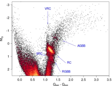
Fig. 10. Gaia HRD of low-extinction nearby giants: $ > 2 mas (500 pc),E(B−V) <0.015 andMG <2.5 (29 288 stars), with labels to the features discussed in the text.
The most prominent feature of the giant branch is the Red Clump (RC in Fig.10, aroundGBP−GRP=1.2,MG=0.5 mag).
It corresponds to low-mass stars that burn helium in their core (e.g.Girardi 2016). The colour of core-helium burning stars is strongly dependent on metallicity and age. The more metal-rich, the redder, which leads to this red clump feature in the local HRD. For more metal-poor populations, these stars are bluer and lead to the horizontal-branch (HB) feature that is clearly visible in globular clusters (Fig.11).
The secondary red clump (SRC in Fig.10, around GBP− GRP= 1.1,MG=0.6) is more extended in its bluest part to fainter magnitudes than the red clump. It corresponds to younger more massive red clump stars (Girardi 1999) and is therefore mostly visible in the local HRD (Fig.6c). Core-helium burning stars that are even more massive are more luminous than the red clump and lie still on the blue part of it, leading to a vertical structure that is sometimes called the Vertical Red Clump (VRC in Fig.10).
On the red side and fainter than the clump lies the RGB bump (RGBB in Fig.10). This bump is caused by a brief interruption of the stellar luminosity increase as a star evolves on the red giant branch by burning its hydrogen shell, which creates an accumu- lation of stars at this HRD position (e.g.Christensen-Dalsgaard 2015). Its luminosity changes more with metallicity and age than the red clump. Brighter than the red clump, at MG∼ −0.5, lies the AGB bump (AGBB in Fig.10), which corresponds to the start of the asymptotic giant branch (AGB) where stars are burning their helium shell (e.g.Gallart 1998). The AGB bump is much less densely populated than the RGB bump. It is also clearly visible in the HRD of 47 Tuc (Fig.11a).
The globular clusters in Fig.11clearly illustrate the diversity of the HB morphology. Some have predominantly blue HB (NGC 6397), some just red HB (NGC 104), and some a mixed HB showing bimodal distribution (NGC 5272 and NGC 6362).
The HB morphology is explained in the framework of the multiple populations; it is regulated by age, metallicity, and first/second generation abundances (Carretta et al. 2009).
NGC 6362 is the least massive globular that presents multiple populations.Mucciarelli et al.(2016) concluded that most of the stars that populate the red HB are Na poor and belong to the first generation, while the blue side of the HB is populated by the Na-rich stars belonging to the second generation. The same kind of correlation is shown in general by the globular clusters. We
quote among others the studies of 47 Tuc (Gratton et al. 2013) and NGC 6397 (Carretta et al. 2009). The role of the He abun- dances is still under discussion (Marino et al. 2014; Valcarce et al. 2016). He-enhanced stars are indeed expected to populate the blue side of the instability strip because they are still O depleted and Na enhanced, as observed in the second-generation stars. How significant the He enhancement is still unclear.
Figure 3 shows that the globular cluster HB can extend towards the extreme horizontal branch (EHB) region. They are in the same region of the HRD as the hot subdwarfs, which creates a clump atMG= 4 andGBP−GRP=−0.5 that is well vis- ible in Figs.1 and5. These stars are also nicely characterised in terms of variability, including binary-induced variability, in Gaia Collaboration(2018b). These hot subdwarfs are considered to be red giants that lost their outer hydrogen layers before the core began to fuse helium, which might be due to the interaction with a low-mass companion, although other processes might be at play (e.g.Heber 2009).Gaia will allow detailed studies of the differences between cluster and field hot subdwarfs.
4.4. Planetary nebulae
At the end of the AGB phase, the star has lost most of its hydro- gen envelope. The gas expands while the central star first grows hotter at constant luminosity, contracting and fusing hydrogen in the shell around its core (post-AGB phase), then it slowly cools when the hydrogen shell is exhausted, to reach the white dwarf phase. This planetary nebulae phase is very short, about 10 000 yr, and is therefore quite difficult to observe in the HRD.
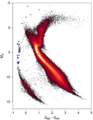
TheGaiaDR2 contains many observations of nearby planetary nebulae as their expanding gas create excess flux over the mean sky background that triggers the on-board detection. We here wish to follow the route of the central star in the HRD. While some central planetary nebula stars are visible in the Galactic Pole HRD (Fig.12), post-AGB stars are too rare to appear in this diagram. We used catalogue compilations to highlight the position of the two types in theGaiaHRD.
We used theKerber et al.(2003) catalogue of Galactic plan- etary nebulae, selecting only sources classified as central stars that are clearly separated from the nebula. With a cross-match radius of 100 and using all our filter criteria of Sect.2.1, only four stars remain. We therefore relaxed the extinction criteria to E(B−V)<0.05 and the parallax relative uncertainty toσ$/$ <
20%, leading to 23 stars.
For post-AGB stars, we used the catalogue ofSzczerba et al.
(2007) and the 2MASS identifier provided for the cross-match.
We selected only stars that are classified as very likely post- AGB objects. Here we also relaxed the extinction criteria to E(B−V)<0.05 and the parallax relative uncertainty toσ$/$ <
20%, leading to 11 stars.
While some outliers are seen in Fig.12, either due to cross- match or misclassification issues, the global position of these stars in the HRD closely follows the expected track from the AGB to the white dwarf sequence. We note that this path crosses the hot subdwarf region we discussed in the previous section.
5. White dwarfs
The Sloan Digital Sky Survey (SDSS,Ahn et al. 2012) has pro- duced the largest spectroscopic catalogue of white dwarfs so far (e.g.Kleinman et al. 2013). This data set has greatly aided our understanding of white dwarf classification and evolution. For example, it has allowed determining the white dwarf mass dis- tribution for large statistical samples of different white dwarf
Fig. 11.Several globular clusters selected to show a clearly defined and very different horizontal branch, sorted by decreasing metallicity.Panel a:
NGC 104 (47 Tuc),panel b: NGC 6362,panel c: NGC 5272, andpanel d: NGC 6397.
Fig. 12. North Galactic Pole HRD (b > 50◦, 2 077 925 stars) with literature central planetary nebula stars (blue) and post-AGB stars (magenta).
spectral types. However, much of this work is model dependent and relies upon theoretical mass-radius relationships and stel- lar atmosphere models, whose precision has only been tested in a limited way. These tests have been limited by the relatively small number of white dwarfs for which accurate parallaxes are available (e.g. Provencal et al. 1998) and by the precision of the parallaxes for these faint stars. This work was updated using theGaiaDR1 catalogue (Tremblay et al. 2017), which included more stars, but the uncertainties remain too large to constrain the theoretical mass-radius relations. Only in a few cases, where the white dwarf resides in a binary system, have mass radius measurements begun to approach the accuracy required to constrain the core composition and H layer mass of individual stars (e.g.Barstow et al. 2005;Parsons et al. 2017;Joyce et al.
2017). Even then, some of these white dwarfs may not be rep- resentative of the general population because common envelope
Fig. 13.GaiaHRD of white dwarfs withσ$/$ <5% (26 264 stars), with letter labels to the features discussed in the text.
evolution may have caused them to depart from the normal white dwarf evolutionary paths.
The publication of Gaia DR2 presents the opportunity to apply accurate parallaxes, with uncertainties of 1% or smaller, to the study of white dwarf stars. The availability of these data, coupled with the accurateGaiaphotometry, yields the absolute magnitude, with which the white dwarfs can be clearly located in the expected region of the HRD (Figs. 5 and6). Figure13 shows the white dwarf region of the HRD alone. This sample was selected with GBP−GRP < 2 and G−10+5 log10$ >
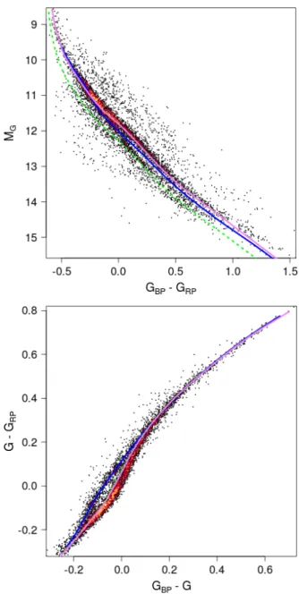
10+2.6 (GBP−GRP) and by applying the filters described in Sect.2, including the low-extinctionE(B−V)<0.015 criterion, but with a stronger constraint on the parallax relative uncertainty of 5%. This yields a catalogue of 26 264 objects. We over- plot in Fig.14white dwarf evolutionary models3for C/O cores (Holberg & Bergeron 2006; Kowalski & Saumon 2006;
Tremblay et al. 2011; Bergeron et al. 2011) with colours com- puted using the revisedGaiaDR2 passbands (Evans et al. 2018).
Several features are clearly visible in Fig.13. First there is a clear main concentration of stars that is distributed continuously
3 http://www.astro.umontreal.ca/~bergeron/
CoolingModels
Fig. 14.GaiaHRD of white dwarfs withσ$/$ <5% andσGBP<0.01 andσGRP <0.01 (5 781 stars) overlaid with white dwarf evolutionary models. Magenta: 0.6Mpure H; green dashed: 0.8 Mpure H; and blue: 0.6Mpure He.Panel a: HRD.Panel b: colour–colour diagram.
from left to right in the diagram (A) and coincides with the 0.6 M hydrogen evolutionary tracks (in magenta). This is expected because the white dwarf mass distribution peaks very strongly near 0.6 M(Kleinman et al. 2013). Interestingly, the concentration of white dwarfs departs from the cooling tracks towards the red end of the sequence.
Just below the main 0.6Mconcentration of white dwarfs is a second, separate concentration (B)that seems to be sepa- rate from the 0.6 M peak atGBP−GRP ∼ −0.1 before again merging byGBP−GRP∼0.8. At the maximum separation, this concentration is roughly aligned with the 0.8Mhydrogen white dwarf cooling track (in green), which is not expected. While the SDSS mass distribution (Kleinman et al. 2013) shows a significant upper tail that extends through 0.8 M and up to almost 1.2M, there is no evidence for a minimum between 0.6 and 0.8 Mlike that seen in Fig.14a. A mass difference should therefore not lead to this feature. However, for a given mass, the evolutionary tracks for different compositions (DA: hydrogen
and DB: helium) and envelope masses are virtually coincident at the resolution of Fig.14in the theoretical tracks, leading to no direct interpretation from the tracks in the HRD alone, but we describe below a different view from the colour–colour relation and the SDSS comparison.
A third, weaker concentration of white dwarfs in Fig.13lies below the main groups(Q). It does not follow an obvious evolu- tionary constant mass curve, which would be parallel to those shown in the plot. Beginning at approximately MG = 13 and GBP−GRP =−0.3, it follows a shallower curve that converges with the other concentrations nearGBP−GRP=0.2.
White dwarfs are also seen to lie above the main concentra- tion A. This can be explained as a mix between natural white dwarf mass distributions and binarity (see Fig.8).
Selecting only the most preciseGBP andGRP photometry (σGBP <0.01 andσGRP <0.01), we examined the colour–colour relation in Fig.14b. The sequence is also split into two parts in this diagram. We verified that the two splits coincide, meaning that the stars in the lower part of Fig.14a lie in the upper part of Fig.14b. The mass is not expected to lead to significant dif- ferences in this colour–colour diagram, and the theoretical tracks coincide with the observed splits, pointing towards a difference between helium and hydrogen white dwarfs. It also recalls the split in the SDSS colour–colour diagram (Harris et al. 2003).
WhileGaiaidentifies white dwarfs based on their location on the HRD, SDSS white dwarfs were identified spectroscopically, providing further information on the spectral type,Teff, and logg as well as a classification. Therefore we cross-matched the two data sets to better understand the features observed in Fig.14.
We obtained a catalogue of spectroscopically identified SDSS white dwarfs from the Montreal White Dwarf Database4 (Dufour et al. 2017) by downloading the whole catalogue and then filtering for SDSS identifier, which yielded 28 797 objects.
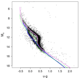
Using the SDSS cross-match provided in the Gaia archive (Marrese et al. 2018), we found that there are 22 802 objects in common and 5 237 satisfying all the filters described in Sect.2.1 and with single-star spectral type information. Figure15shows the SDSS u−g colour magnitude for the sample with the absolute u magnitude calculated using theGaia parallax. The distribution is clearly bifurcated. Evolutionary tracks for H and He atmospheres (0.6M) are overplotted in the figure, indicat- ing that this is due to the different atmospheric compositions.
The Gaia counterparts of these SDSS white dwarfs are quite faint, and therefore the features seen in Fig. 14a are less well visible in this sample because of the larger noise in the paral- laxes and the colours. Still, it allowed us to verify that the split of the SDSS white dwarfs corresponds to the location of theGaia splits in Fig. 14. The narrower filter bands of SDSS are more sensitive to atmospheric compositions than the broad BP and RPGaiabands. In particular, the u-band fluxes of H-rich DA white dwarfs are suppressed by the Balmer jump at 364.6 nm, which reddens the colours of these stars. The Balmer jump is in the wavelength range where theGaiafilters calibrated for DR2 differ most from the nominal filters (Evans et al. 2018), which explains the importance of using tracks that are updated to the DR2 filters for the white dwarf studies instead of the nominal tracks provided byCarrasco et al.(2014).
Figure16shows the colour-magnitude diagrams in theGaia and SDSS photometry bands, overlaid with the white dwarfs for specific spectral types. The locations of the various spectral types correspond well to the expected colours arising from their effective temperatures. For example, DQ (carbon), DZ (metal
4 http://www.montrealwhitedwarfdatabase.org/