2018 14th International Conference on Natural Computation, Fuzzy Systems and Knowledge Discovery (ICNC-FSKD 2018)
Automatic segmentation of low-grade brain tumor using a random forest classifier and Gabor features
Zs´ofia Szab´o∗, Zolt´an Kap´as∗, L´aszl´o Lefkovits∗, ´Agnes Gy˝orfi∗, S´andor M. Szil´agyi†‡ and L´aszl´o Szil´agyi∗‡
∗Computational Intelligence Research Group (CIRG), Sapientia University, Tˆırgu Mures¸, Romania E-mail: lalo@ms.sapientia.ro
†Department of Informatics, Petru Maior University, Tˆırgu Mures¸, Romania
‡Dept. of Control Engeneering and Information Technology Budapest University of Technology and Economics, Budapest, Hungary
Abstract—Computerized tumor detection and segmentation algorithms are developed to assist the work medical staff at the diagnosis or therapy planning. This paper presents a procedure trained to segment low-grade gliomas in multispectral volumetric MRI records. The proposed solution employs a random forest classifier based on 104 morphological and Gabor wavelet features.
A neighborhood-based post-processing was designed to regularize the output of the classifier. The current version of our system was trained and tested using all 54 low-grade tumor volumes from the MICCAI BRATS 2016 database. The achieved accuracy is characterized by an overall mean Dice score of83.8%, sensitivity
>85%, and specificity>98%. The proposed method is likely to detect all gliomas of2cmdiameter.
Index Terms—Image segmentation, tumor detection, magnetic resonance imaging, random forest, Gabor wavelet.
I. INTRODUCTION
Most tumors are diagnosed after its symptoms convince the patients to go to the doctor. In this case the tumor is detected in a certain advanced stage, when the chances of survival are reduced. The development of imaging devices and computers enable us to elaborate solutions that would allow for regular screening of a larger population and tracing most tumors in an earlier phase. In such conditions, automated algorithms and procedures are needed, which can efficiently and reliably detect and localize the tumor. Beside establishing the diagnosis, the automatic segmentation and quantitative analysis can assist therapy planning and evolution tracking of the tumor. However, automatic tumor segmentation is not only utmost important task, but also a very challenging one, because of the high variety of anatomical structures and low contrast of current imaging techniques, which make the difference between normal regions and the tumor hardly recognizable for the human eye [1].
Magnetic resonance imaging (MRI) is the preferred imaging device in brain tumor screening, due to its better contrast and relatively fine resolution. However, it also bears difficulties like the possible presence of intensity inhomogeneity [2], and the relative intensity values that vary from device to device and from patient to patient. The MICCAI Brain Tumor Segmen- tation Challenge, organized yearly since 2012, intensified the research in this topic and led to several important solutions, which are usually assisted by the use of prior information, and employ various image processing and pattern recognition
methodologies. Asman et al [3] applied a non-parametric intensity analysis in combination with a segmentation based on multiple atlases. Ghanavati et al [4] provided a solution using the AdaBoost classifier to distinguish tumor voxels from normal ones using features based on intensity, texture, and symmetry. Hamamci et al [5] proposed a cellular automata driven method that produces segmentation based on level sets.
Sachdeva et al [6] deployed a content based active contour model relying on intensity and texture features extracted from the histogram and co-occurrence matrix of the MRI data. Njeh et al [7] introduced a graph cut based solution that performs distribution matching, which is highly efficient because of using rather global than pixelwise information. Zhang et al [8] proposed a support vector machine based procedure to follow the evolution of brain tumors over time. Tustison et al [9] combined random forests with symmetry based features to segment brain tumors. Szil´agyi et al [10] provided a semi-supervised framework for the fuzzy c-means clustering algorithm to produce accurately segmented tumors. Kanas et al [11] combined a clustering based preprocessing with a multi- parametric random walker segmentation. Havaei et al [12]
developed an automatic brain tumor segmentation procedure based on deep neural networks that exploits both local and global contextual features simultaneously. Pereira et al [13]
proposed a convolutional neural network solution exploiting small kernels and successfully applied it for brain tumor segmentation. Menze et al [14] combined a Gaussian mixture model with the expectation maximization (EM) algorithm to achieve an accurate segmentation. Another Gaussian mixture based accurate solution was given by Juan-Albarrac´ın et al [15]. Islam et al [16] employed multifractional Brownian mo- tion features to provide patient-independent characterization of tumor tissues and applied the AdaBoost algorithm for tissue segmentation. Shin et al [17] proposed deep convolutional neural networks and successfully combined it with transfer learning. Huang et al [18] provided a brain tumor segmen- tation framework employing local independent projection- based classification. Lˆe et al [19] proposed a brain tumor segmentation procedure based on a tumor growth model. Pinto et al [20] employed extremely random trees to provide a hierarchical solution to the low-grade glioma segmentation problem. Zaouche et al [21] provided a semi-supervised low-
grade glioma segmentation based on specially designed spatial edge filters and maximum likelihood optimization. For further information on current brain tumor segmentation techniques, there are available recent reviews [1], [22], [23], [24], [25].
In a previous paper [26] we have presented a preliminary study on the use of random forests in the detection and segmentation of high-grade gliomas. The feature vector char- acterizing each voxel contained 16 values, including minimum, maximum, and median values computed from the neighbor- hood of the voxel. The procedure proposed in that study was evaluated using the 220 high-grade tumor volumes from the MICCAI BRATS 2016 data set. The best overall Dice Score was found 81%. As a further development of our previous algorithm, in this paper we propose a random forest solution trained and tested using 104-element feature vectors that include various computed morphological and Gabor wavelet features. Our main goal in this paper is to accurately separate the whole tumor from the normal tissues in each low-grade tumor volume of the MICCAI BRATS 2016 database.
The rest of this paper is structured as follows: Section II gives details on the proposed methodology. Section III exhibits and discusses the achieved results. Finally, Section IV concludes the investigation.
II. MATERIALS ANDMETHODS
Our goal was to elaborate an accurate segmentation proce- dure for low-grade brain tumors based on a machine learning algorithm. This paper presents preliminary results obtained using a random forest approach, combined with histogram normalization, Gabor feature extraction for texture characteri- zation, and a neighborhood-based post-processing. The trees of the random forest are trained to separate the whole tumor from normal tissues. The structure of the elaborated segmentation procedure is presented in Fig. 1.
A. BRATS data sets
Multimodal MR image data involved in this study was obtained from the MICCAI 2016 Challenge on Multimodal Brain Tumor Segmentation [27]. This database contains fully anonymized image volumes originating from four institutions.
The image database consists of multi-contrast MR scans of 274 glioma patients, out of which 220 having high-grade and 54 having low-grade glioma lesions. For each patient, multimodal (T1, T2, FLAIR, and post-Gadolinium T1) MR images were recorded and linearly co-registered to the T1 contrast image. Additionally, all data volumes were skull stripped, and interpolated to 1mmisotropic resolution. Each record contains approximately 1.5 millions of true tissue voxels, out of which up to 20% can be positive. All voxels are provided with manual annotation produced by human expert.
Although the four observed features of each voxel bear a lot more information than any one of them, there is an acute need to extend the feature vectors with further computed features.
B. Histogram normalization
A major drawback of MR imaging consists in the lack of a standard scale of image intensities. This is why we need to
map the histogram of each data channel of BRATS volumes onto a uniform scale. Although literature contains various recommendation is this issue [28], [29], we opted to employ a simple linear transform x → αx +β to all intensities, where parameters α and β were established separately for each volume and each data channel such a way that the 25-percentile and 75-percentile values became 600 and 800, respectively. Further on, a minimum and a maximum intensity barrier was enforced at 200 and 1200, respectively.
C. Computed features
A total number of 100 computed features were added to the feature vector describing each voxel, according to the inventory given in Table I. For each of the four observed intensities (T1, T2, T1C, FLAIR), six average, five median, one minimum, one maximum, four gradient values, and further 8 Gabor features were extracted. All computed feature values were linearly scaled into the[200,1200]interval. This way, to- gether with the four observed features, each voxel is described by a 104-element feature vector. These feature vectors are used by the classification stage of the proposed segmentation procedure.
D. Missing data
We considered that the region of interest (ROI) in the BRATS volumes includes all voxels that have at least one nonzero value in any of the observed data channels. Zero in- tensities within the observed features of any voxel belonging to the ROI were considered missing values. Missing values were replaced by the mean intensity value of existing neighbors within the 26-element immediate spatial neighborhood, or the grand mean of the given data channel whenever no neighbors with correct intensity were found in the neighborhood.
E. Binary decision trees
Binary decision trees (BDT) of unlimited depth can describe any hierarchy of crisp (non-fuzzy) two-way decisions [30].
Given an input data set of vectors X = {x1,x2, . . . ,xn}, where xi = [xi,1, xi,2, . . . , xi,m]T, a BDT can be employed to learn the classification that corresponds to any set of labels Λ ={λ1, λ2, . . . , λn}. The classification learned by the BDT can be perfect if there are no identical training vectors with different labels, that is, xi = xj implies λi = λj, ∀i, j ∈ {1,2, . . . , n}. The BDT is built during the training process.
Initially the tree consists of a single node, the root, which has to make a decision regarding all n train data vectors. If not all n vectors have the same label, which is likely to be so, then the set of data is not homogeneous, and there is a need for a separation. The decision will compare a single chosen feature, the one with index k (1 ≤ k ≤ m), of the input vectors with a certain threshold α, and the comparison will separate the vectors into two subgroups: those with xi,k < α (i= 1. . . n), and those withxi,k≥α(i= 1. . . n). The root will then have two child nodes, each corresponding to one of the possible outcomes of the above decision. The left child will further classify those n1 input vectors, which satisfied
Histogram normalization
Feature extraction
Definition of train and test data
Data sampling for each tree in random forest
Apply trained forests to testing data
Training decision trees
OOB based evaluation
Neighborhood based postprocessing
Result evaluation
?
?
?
?
- - -
- -
BRATS data
Test data Train data
Trained forests
Segmented volumes
Post-processed segmented volumes
TP, TN, FP, FN TPR, TNR, DS
...training testing
Fig. 1. Block diagram of the segmentation procedure.
TABLE I
INVENTORY OF COMPUTED FEATURES. ALL4DATA CHANNELS WERE INVOLVED EQUALLY. Neighborhood Average Maximum Minimum Median Gradient Gabor Total
3×3×3 4 4 4 12
3×3 4 4 8
5×5 4 4 8
7×7 4 4 16 24
9×9 4 4 8
11×11 4 4 32 40
Total 24 4 4 20 16 32 100
the former condition, while the right child thosen2 ones that satisfied the latter condition. Obviously, we haven1+n2=n withn1>0andn2>0. For both child nodes, the procedure is the same as it was for the root. When at a certain point of the learning algorithm, all vectors being classified by a node have the same labelλp, then the node is declared a leaf node, which is attributed to the class with index p. Another case when a node is declared leaf node is when all vectors to be separated by the node are identical, so there is no possible condition to separate the vectors. In this case, the label of the node is decided by the majority of labels, or if there is no majority, a label should be chosen from the present ones. In our application, this kind of rare leaves are labeled as tumor.
The separation of a finite set of data vectors always termi- nates in a finite number of steps. The maximum depth of the tree highly depends on the way of establishing the separation condition in each node. Our application uses an entropy based criterion to choose the separation condition. Whenever a node has to establish its separation criterion for a subset of vectors X ⊆ X containing n items with 1 < n≤ n, the following algorithm is performed:
1) Find all those features which have at least 2 different values inX.
2) Find all different values for each feature and sort them in increasing order.
3) Set a threshold candidate at the middle of the distance between each consecutive pair of values for each feature.
4) Choose that feature and that threshold, for which the entropy-based criterion
E=n1logn1
n +n2logn2
n (1)
gives the minimum value, where n1 (n2) will be the cardinality of the subset of vectorsX1 (X2), for which the value of the tested feature is less than (greater or equal than) the tested threshold value.
After having the BDT trained, it can be applied for the classification of test data vectors. Any test vector is first fed to the root node, which according to the stored condition and the feature values of the vector, decides towards which child node to forward the vector. This strategy is followed then by the chosen child node, and the vector will be forwarded to a further child. The classification of a vector terminates at the moment when it is forwarded to a leaf node of the tree.
The test vector will be attributed to the class indicated by the labeling of the reached leaf node.
F. The random forest
Binary decision trees were trained to separate tumor voxels from negative ones. In case of the BRATS low-grade tumor data set, we had a total number of 72.2 million negative and 5.46 million positive voxels. As a first step, randomly selected 88% of the negative voxels were eliminated and the remaining 12% kept for the training and testing process.
Random forests were trained according to the following parameters:
1) The number of trees in the forest denoted by nT. This parameter was usually set to 255, but experiments were performed with other values as well.
2) The number of data vectors used to train each tree of the forest, denoted bynP. Typical values of this parameter ranged from 10 thousand to 500 thousand.
3) The rate (percentage) of negative labeled data within the training set, denoted by pn. It is likely to achieve best performance around pn = 93%, which is the true rate of negatives within the BRATS LG volumes.
Ideal parameter settings were identified using the so-called out-of-bag (OOB) data, as recommended by Breiman in [31].
Testing on OOB data allowed us to preselect those forests that were likely to produce high accuracy, and discard those that were prone to severe misclassifications. The best performing trees achieved 93-94% accuracy, while the most accurate forests scored 95-96% in labeling the OOB data.
At classification, all voxels from the test volumes receive a vote (label) from each BDT of the random forest. The final labeling of voxels is decided by the majority of votes.
G. Post-processing
A posterior relabeling scheme was implemented as follows.
The input data of the post-processing step consisted in the labels provided by the random forest to all voxels in the test volume. For each voxel, the number of tumor labeled neighbors (νT) and the number of all neighbors (νAll) were extracted, using a predefined neighborhood. The final label of a voxel was set to tumor if and only ifνT/νAll> θ. The overall optimal value of the threshold was established using the OOB data and was found as θ= 0.34. The ideal neighborhood to be employed in post-processing was identified as the cubic 11×11×11sized one.
H. Evaluation of accuracy
We employed the Dice score (DS) as the main indicator of accuracy, defined as
DS = 2×TP
2×TP + FP + FN ∈[0,1] , (2) whereTP,FP, andFNstand for the number of true positives, false positives, and false negatives, respectively. Fine accuracy is reflected by DS values close to 1, but in this brain tumor segmentation problem, DS values around0.94are considered ideal [27], due to inter-rater differences that are present in the ground truth. Further on, sensitivity (or true positive rate, TPR) defined as
TPR = TP
TP + FN , (3)
and specificity (or true negative rate) defined as TNR = TN
TN + FP (4)
Fig. 2. Overall Dice Score plotted against the number of voxels used to train each decision tree of the random forest, at various values of the negative train data ratepn. These results were obtained usingnT= 255trees in each random forest.
Fig. 3. Overall Dice Score plotted against the negative train data ratepn, at various values of the number of voxelsnP used to train each decision tree of the random forest. These results were obtained usingnT = 255trees in each random forest.
were used as secondary accuracy indicators, whereTNrepre- sents the number of true negatives.
If we denote by TPi, TNi, FPi, and TPi, the true/false positives/negatives obtained at testing volume number i (i= 1. . . p, where p = 54 is the number of volumes), then we define average Dice Score as
DS =f 1 p
p
X
i=1
DSi=1 p
p
X
i=1
2×TPi
2×TPi+ FPi+ FNi
, (5)
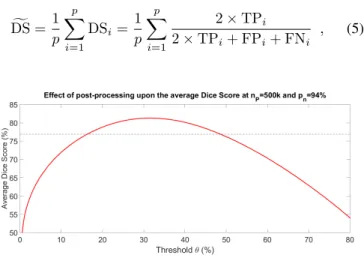
Fig. 4. The effect of post-processing: the average Dice Score obtained at nP = 500k and pn = 94%, plotted against the neighborhood threshold θ. The horizontal dashed line indicates the average Dice Score before post- processing. Post-processing can provide an up to 4%improvement of the accuracy when usingθ∈[30%,35%].
Fig. 5. The effect of post-processing upon the segmentation accuracy of individual volumes: (left) Dice Scores DS1. . .DSp before and after post- processing, plotted in increasing order; (right) Dice Scores obtained for individual image volumes, after post-processing vs. before post-processing.
Neighborhood parameter was set toθ= 34%.
Fig. 6. The effect of post-processing upon the segmentation accuracy of individual volumes: (left) sensitivity before and after post-processing, plotted in increasing order; (right) sensitivity obtained for individual image volumes, after post-processing vs. before post-processing.
and overall Dice Score as:
DS =
2×
p
P
i=1
TPi 2×
p
P
i=1
TPi+
p
P
i=1
FPi+
p
P
i=1
FNi
. (6)
Similarly, we will compute overall and average values for the sensitivity (TPR,TPR) and the specificity (TNR,g TNR).g
III. RESULTS ANDDISCUSSION
All 54 low-grade tumor volumes from the BRATS 2016 data set were involved in the evaluation of the proposed methodology. Volumes were randomly separated into two equal groups. Random forests were trained with data from one of the groups and tested on data from the other group. This way all volumes were used as train and test data in turns.
The rate of positive voxels within the whole data set is approximately 7%. All positive voxels of the train volumes, and a randomly selected 12%-subset of negative voxels were used as training data set. For the training of each random tree,nP voxels were randomly selected from the training data set such a way, that pn percent of them were negatives and the rest of the voxels were positive. During the evaluation of the proposed algorithm, nP values ranged between 10k and 500k, while the percentage of negative train voxels pn
varied between 85% and 95%. Ratios lower than 85% were
Fig. 7. The Dice Scores obtained for each volume before post-processing, plotted against the actual size of the tumor. The dashed lines indicates the trend extracted via linear regression.
Fig. 8. The Dice Scores obtained for each volume after post-processing, plotted against the actual size of the tumor. The dashed lines indicates the trend extracted via linear regression.
also used, but they led to too many false positives in case of any test volume. A number ofnT = 255trees were trained for each test case. This enabled us to analyze the relation between the accuracy of the proposed algorithm and the number of necessary trees in the random forest.
Figures 2 and 3 exhibit the obtained overall Dice ScoreDS in case of various values of train data sizenP and percentage of negative train data pn. The accuracy visibly improves as the train data size grows, but this phenomenon slows down at nP >200kvoxels. Considering that bigger train data sets lead to deeper decision trees and consequently to longer processing time, there must be a compromise in the question of train data size. On the other hand, the optimal percentage of negative data is similar to the true rate of negative in all the image volumes. At train data sizes up tonP = 10k,pn= 92%was found optimal. Train data sizes ofnP ∈ {20k,30k,50k,100k}
resulted in optimal negative data ratepn = 93%, while larger data sizes performed best atpn = 94%. In every setting, we were able to achieve overall Dice Scores above82%, while the best accuracy ofDS = 83.8%was achieved atnP = 500kand pn = 94%. Global accuracy indicators obtained atnT = 255 trees in the random forest are presented in Table II.
Figure 4 presents the global effect of the post-processing upon the average Dice Score, depending on the neighborhood thresholdθ. Accuracy reaches its maximum somewhere in the intervalθ∈[30%,35%], but there is a wide range of θwhere the effect of post-processing is beneficial.
Figure 5 presents the effect of the proposed post-processing.
TABLE II
MAIN ACCURACY INDICATORS
Post-processing OverallDS AverageDSf Median DS DS>80% DS>85% DS>90%
Before 81.0% 77.0% 81.0% 30 of 54 16 of 54 6 of 54
After 83.8% 81.3% 84.6% 42 of 54 26 of 54 12 of 54
Post-processing OverallTPR AverageTPRg Median TPR OverallTNR AverageTNRg Median TNR
Before 76.7% 77.0% 81.0% 99.03% 99.04% 99.33%
After 84.8% 81.3% 84.6% 98.64% 98.64% 98.84%
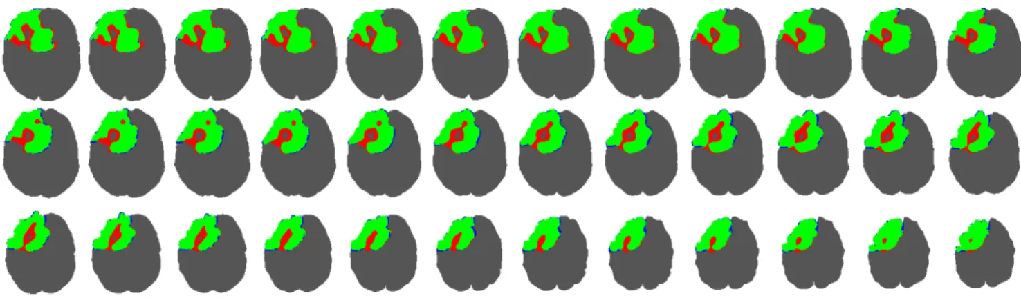
Fig. 9. Thirty-six consecutive slices from an identified tumor. Green pixels represent true positives, blue and red ones stand for false positives and false negatives, respectively. The Dice Score for this volume was above 94%.
Fig. 10. Thirty-six consecutive slices from an identified tumor. Green pixels represent true positives, blue and red ones stand for false positives and false negatives, respectively. The Dice Score for this volume was 82.5%.
The left side exhibits the main accuracy indicator for each individual volume, before and after post-processing. The indi- cator values were sorted in increasing order for better visibility.
On the right side it plots the individual Dice scores for each volume after post-processing vs. before post-processing, indicating that post-processing had a significant beneficial effect in a great majority of the cases, and only 10% of the volumes were slightly pushed toward worse accuracy. Figure 6 presents the effect of post-processing upon sensitivity, using the very same concept.
Figures 7 and 8 plot the individual Dice scores obtained for each volume vs. the size of the tumor, without post-processing and with post-processing, respectively. The identified linear trends show that the strongest effect of post-processing occurs in case of small tumors.
Figure 9 exhibits the segmentation result of 36 consecutive slices from a low-grade tumor volume. Most tumor pixels were accurately identified in this case, as we can only see a few false negatives beside the true positives indicated by black pixels. This is one of the cases that were segmented with high accuracy. A worse, but still acceptable case is shown in Fig. 10.
The segmentation of a single volume ranges between 60 and 75 seconds, when executed on a single core of a PC with i7 processor running at 3.4 GHz frequency, which can be reduced below 20 seconds when executed in parallelized version on four cores. The largest computational burden represents the extraction of the 100 extra features for the approximately 1.5 million voxels of the volume.
The overall Dice score of 83.8% allows us to detect the presence of the tumor in a great majority of cases. However,
the accuracy indicators can be further improved the following ways:
1) Using further texture features extracted from the neigh- borhood of each voxel.
2) Employing an effective feature selection scheme to eliminate useless features.
3) Implementing a more complex post-processing that in- vestigates the contiguous ensembles of detected tumor voxels and discard small ones.
An objective comparison with existing methods enumerated in Section I is not an easily accomplishable task, as not all of them used the BRATS data set for evaluation, and even those which did, they did not evaluate all the 54 available low- grade tumor volumes. With respect to the methods involved in the comparison in [20], our proposed methodology seems competitive, and it will improve with the implementation of the above listed ideas.
IV. CONCLUSION
This paper presented an automatic low-grade tumor detec- tion and segmentation algorithm employing random forests of binary decision trees, in its intermediate stage of imple- mentation. The proposed methodology reliably detects low- grade tumors of 2cm diameter. It is likely to obtain finer segmentation accuracy in the future via implementing some of the above mentioned further development ideas. We will also concentrate on differentiating among the parts of the whole tumor (edema, tumor core, necrosis, active tumor), according to the grand truth provided by the BRATS database.
ACKNOWLEDGMENT
This research was partially supported by the Sapientia Insti- tute for Research Programs (KPI). The work of Zs´ofia Szab´o was additionally supported by the Accenture Research Schol- arship. The work of S´andor M. Szil´agyi and L´aszl´o Szil´agyi was additionally supported by the Hungarian Academy of Sciences through the J´anos Bolyai Fellowship Program.
REFERENCES
[1] N. Gordillo, E. Montseny and P. Sobrevilla, “State of the art survey on MRI brain tumor segmentation,”Magnetic Resonance Imaging, vol. 31, pp. 1426–1438, 2013.
[2] U. Vovk, F. Pernu˘s and B. Likar, “A review of methods for correction of intensity inhomogeneity in MRI,” IEEE Transactions on Medical Imaging, vol. 26, pp. 405–421, 2007.
[3] A. J. Asman and B. A. Landman, “Out-of-atlas labeling: a multi-atlas approach to cancer segmentation,” IEEE International Symposium on Biomedical Imaging(ISBI 2012, Barcelona), pp. 1236–1239, 2012.
[4] S. Ghanavati, J. Li, T. Liu, P. S. Babyn, W. Doda and G. Lampropoulos,
“Automatic brain tumor detection in magnetic resonance images,”IEEE International Symposium on Biomedical Imaging(ISBI 2012, Barcelona), pp. 574–577, 2012.
[5] A. Hamamci, N. Kucuk, K. Karamam, K. Engin and G. Unal, “Tumor- Cut: segmentation of brain tumors on contranst enhanced MR images for radiosurgery applicarions,”IEEE Transactions on Medical Imaging, vol.
31, pp. 790–804, 2012.
[6] J. Sahdeva, V. Kumar, I. Gupta, N. Khandelwal and C. K. Ahuja, “A novel content-based active countour model for brain tumor segmentation,”
Magnetic Resonance Imaging, vol. 30, pp. 694–715, 2012.
[7] I. Njeh, L. Sallemi, I. Ben Ayed, K. Chtourou, S. Lehericy, D. Galanaud and A. Ben Hamida, “3D multimodal MRI brain glioma tumor and edema segmentation: a graph cut distribution matching approach,”Computerized Medical Imaging and Graphics, vol. 40, pp. 108–119, 2015.
[8] N. Zhang, S. Ruan, S. Lebonvallet, Q. Liao and Y. Zhou, “Kernel feature selection to fuse multi-spectral MRI images for brain tumor segmentation,”Computer Vision and Image Understanding, vol. 115, pp.
256–269, 2011.
[9] N. J. Tustison, K. L. Shrinidhi, M. Wintermark, C. R. Durst, B. M.
Kandel, J. C. Gee, M. C. Grossman and B. B. Avants, “Optimal symmetric multimodal templates and concatenated random forests for supervised brain tumor segmentation (simplified) with ANTsR,”Neuroinformics, vol.
13, pp. 209–225, 2015.
[10] L. Szil´agyi, L. Lefkovits and B. Beny´o, “Automatic Brain Tumor Seg- mentation in multispectral MRI volumes using a fuzzy c-means cascade algorithm”,Proc. 12th International Conference on Fuzzy Systems and Knowledge Discovery (FSKD 2015, Zhangjiajie, China), pp. 285-291, 2015.
[11] V. G. Kanas, E. I. Zacharaki, C. Davatzikos, K. N. Sgarbas and V.
Megalooikonomou, “A low cost approach for brain tumor segmentation based on intensity modeling and 3D random walker,”Biomedical Signal Processing and Control, vol. 22, pp. 19–30, 2015.
[12] M. Havaei, A. Davy, D. Warde-Farley, A. Biard, A. Courville, Y. Bengio, C. Pal, P. M. Jodoin and H. Larochelle, “Brain tumor segmentation with deep neural networks”,Medical Image Analysis, vol. 35, pp. 18–31, 2017.
[13] S. Pereira, A. Pinto, V. Alves and C. A. Silva, “Brain tumor segmentation using convolutional neural networks in MRI images,”IEEE Transactions on Medical Imaging, vol. 35, pp. 1240–1251, 2016.
[14] B. H. Menze, K. van Leemput, D. Lashkari, T. Riklin-Raviv, E. Geremia, E. Alberts, et al. “A generative probabilistic model and discriminative extensions for brain lesion segmentation – with application to tumor and stroke,”IEEE Transactions on Medical Imaging, vol. 35, pp. 933–946, 2016.
[15] J. Juan-Albarrac´ın, E. Fuster-Garcia, J. V. Manj´on, M. Robles, F. Aparici, L. Mart´ı-Bonmat´ı and J. M. Garc´ıa-G´omez, “Automated glioblastoma segmentation based on a multiparametric structured unsupervised clas- sification,”PLoS ONE, vol. 10(5), e0125143, 2015.
[16] A. Islam, S. M. S. Reza and K. M. Iftekharuddin, “Multifractal tex- ture estimation for detection and segmentation of brain tumors,” IEEE Transactions on Biomedical Engineering, vol. 60, pp. 3204–3215, 2013.
[17] H. C. Shin, H. R. Roth, M. C. Gao, L. Lu, Z. Y. Xu, I. Nogues, J. H. Yao, D. Mollura and R. M. Summers, “Deep nonvolutional neural networks for computer-aided detection: CNN architectures, dataset characteristics and transfer learning,”IEEE Transactions on Medical Imaging, vol. 35, pp. 1285–1298, 2016.
[18] M. Y. Huang, W. Yang, Y. Wu, J. Jiang, W. F. Chen and Q. J. Feng,
“Brain tumor segmentation based on local independent projection-based classification,”IEEE Transactions on Biomedical Engineering, vol. 61, pp. 2633–2645, 2014.
[19] M. Lˆe, H. Delingette, J. Kalpathy-Cramer, E. R. Gerstner, T. Batchelor, J. Unkelbach and N. Ayache, N., “Personalized radiotherapy planning based on a computational tumor growth model,”,IEEE Transactions on Medical Imaging, vol. 36, pp. 815–825, 2017
[20] A. Pinto, S. Pereira, D. Rasteiro and C. A. Silva, “Hierarchical brain tumour segmentation using extremely randomized trees,”Pattern Recog- nition, available online 7 May 2018, doi: 10.1016/j.patcog.2018.05.006 [21] R. Zaouche, A. Belaid, S. Aloui, B. Solaiman, L. Lecornu, D. Ben
Salem and S. Tliba, “Semi-automatic method for low-grade gliomas segmentation in magnetic resonance imaging,”IRBM, vol. 39, pp. 116–
128, 2018.
[22] J. E. Iglesias and M. R. Sabuncu, “Multi-atlas segmentation of biomed- ical images: A survey,”Medical Image Analysis, vol. 24, pp. 205–219, 2015.
[23] S. Mitra and B. Uma Shankar, “Medical image analysis for cancer management in natural computing framework,”Information Sciences, vol.
306, pp. 111–131, 2015.
[24] J. Ker, L. P. Wang, J. Rao and T. Lim, “Deep learning applications in medical image analysis,”IEEE Access, vol. 6, pp. 9375–9389, 2017.
[25] G. Mohan and M. Monica Subashini, “MRI based medical image analysis: Survey on brain tumor grade classification,”Biomedical Signal Processing and Control, vol. 39, pp. 139–161, 2018.
[26] Z. Kap´as, L. Lefkovits, D. Icl˘anzan, ´A. Gy˝orfi, B. L. Iantovics, S.
Lefkovits, S. M. Szil´agyi and L. Szil´agyi, “Automatic brain tumor seg- mentation in multispectral MRI volumes using a random forest approach,”
Proc. Pacific-Rim Symposium on Image and Video Technology(PSIVT 2017, Wuhan),Lecture Notes in Computer Science, vol. 10749, pp. 137–
149, 2018.
[27] B. H. Menze, A. Jakab, S. Bauer, J. Kalpathy-Cramer, K. Farahani, J.
Kirby et al., “The multimodal brain tumor image segmentation benchmark (BRATS),”IEEE Transactions on Medical Imaging, vol. 34, pp. 1993–
2024, 2015.
[28] L. G. Ny´ul, J. K. Udupa and X. Zhang, “New variants of a method of MRI scale standardization,”IEEE Transactions on Medical Imaging, vol.
19, no. 2, pp. 143–150, 2000.
[29] J. D. Christensen, “Normalization of brain magnetic resonance images using histogram even-order derivative analysis,” Magnetic Resonance Imaging, vol. 21, no. 7, pp. 817–820, 2003.
[30] S. B. Akers, “Binary decision diagrams,”IEEE Transactions on Com- puters, vol. C-27, pp. 509–516, 1978.
[31] L. Breiman, “Random forests,” Machine Learning, vol. 45, pp. 5–32, 2001.