MR Image Data Using Random Forest Classifier
?Szabolcs Csaholczi1, David Icl˘anzan1, Levente Kov´acs2, and L´aszl´o Szil´agyi1,2
1 Computational Intelligence Research Group
Sapientia - Hungarian University of Transylvania, Tˆırgu Mure¸s, Romania szabolcscsaholczi55@gmail.com, {iclanzan,lalo}@ms.sapientia.ro
2 University Research, Innovation and Service Center (EKIK) Obuda University, Budapest, Hungary´
{kovacs.levente,szilagyi.laszlo}@nik.uni-obuda.hu
Abstract. The development of brain tumor segmentation techniques based on multi-spectral MR image data has relevant impact on the clin- ical practice via better diagnosis, radiotherapy planning and follow-up studies. This task is also very challenging due to the great variety of tumor appearances, the presence of several noise effects, and the differ- ences in scanner sensitivity. This paper proposes an automatic procedure trained to distinguish gliomas from normal brain tissues in multi-spectral MRI data. The procedure is based on a random forest (RF) classifier, which uses 80 computed features beside the four observed ones, including morphological ones, gradients, and Gabor wavelet features. The inter- mediary segmentation outcome provided by the RF is fed to a twofold post-processing, which regularizes the shape of detected tumors and en- hances the segmentation accuracy. The performance of the procedure was evaluated using the 274 records of the BraTS 2015 train data set. The achieved overall Dice scores between 85-86% represent highly accurate segmentation.
Keywords: magnetic resonance imaging, brain tumor detection, tumor segmentation, random forest.
1 Introduction
Gliomas represent a common malignant brain tumor with low survival rate and short life expectancy. Patients with so-called high-grade (HG) gliomas live fifteen
?This project was supported by the Sapientia Foundation Institute for Scientific Re- search. The work of L. Kov´acs was supported by the European Research Council (ERC) under the European Unions Horizon 2020 research and innovation programme (grant agreement No 679681). The work of L. Szil´agyi was supported by the Hun- garian Academy of Sciences through the J´anos Bolyai Fellowship program, and by the ´UNKP-19-4 New National Excellence Program of the Ministry for Innovation and Technology.
months in average after the diagnosis, while those with low-grade (LG) gliomas can live for several years. In the current clinical practice, most of the times brain tumors are segmented manually, which is time consuming and error prone [1].
With the quickly increasing number of MRI devices deployed in hospitals and the high costs of training human experts, a strong need arising for automatic and reliable tumor detection and segmentation methods. Such algorithms could process the huge amount of acquired MRI data and select those patients which are suspected of having focal lesions in the brain, and consequently assist the medical experts in focusing on serious cases.
Multi-spectral MRI is the most frequently used and preferred medical imag- ing modality in brain tumor detection and segmentation, due to its fine con- trast and the multiple data channels that offer complementary information. The Brain Tumor Segmentation (BraTS) Challenges organized jointly with the MIC- CAI conference, have provided the research community a continuously growing multi-spectral MRI data set of high quality and great challenges [2, 3].
Earlier solutions to the challenge called brain tumor segmentation based on MRI data were summarized by Gordillo et al [4]. Recent solutions usually combine advanced (mostly unsupervised) image segmentation algorithms with semi-supervised supervised classification algorithms that cover the whole arsenal of machine learning techniques, namely: graph cut segmentation algorithm [5], superpixels combined with non-parametric classifiers [6], feature fusion combined with joint label fusion [7], texture feature and kernel sparse coding [8], Gaussian mixture models [9], fuzzy c-means clustering in semi-supervised context [10], fuzzyc-means clustering combined with region growing [11], AdaBoost classifier [12], extremely random trees [13] combined with superpixel level features [14], random forests [15, 16] and ensemble of random forests [17], support vector ma- chines [18], expert systems [19], convolutional neural network [20], deep neural networks [21], generative adversarial networks [22], and tumor growth model [23].
This paper proposes a random forest based brain tumor segmentation proce- dure, including adequate preprocessing and post-processing tasks designed to en- hance the accuracy of segmentation. Preprocessing eliminates noises and handles the spectral differences between various MRI records. Post-processing regularizes the shape of detected tumors and handles the cases with multiple detected le- sions. The MICCAI BraTS 2015 train data set [2, 3] is employed both for training and evaluation purposes.
The rest of the paper is structured as follows: section 2 presents the details of the proposed automatic segmentation procedure, dedicating a subsection to every processing phase. Section 3 evaluates the accuracy of the proposed method, while section 4 concludes the study.
2 Materials and Methods
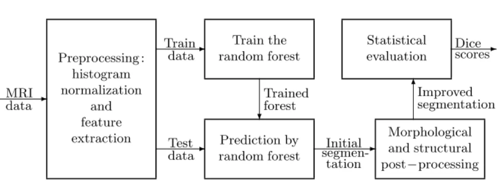
The proposed procedure has the structure shown in Figure 1. It starts with a multiple purpose preprocessing, which is equally applied to all MRI data records.
Statistical evaluation
Morphological and structural post−processing Prediction by
random forest Preprocessing :
histogram normalization
and feature extraction
Train the random forest
-
-
- -
6
? MRI
data
Train data
Test data
Initial segmen-
tation
Improved segmentation
Dice- scores Trained
forest
Fig. 1.The proposed segmentation algorithm.
This is followed by splitting the MRI records to train and test data records from test data records. Train records are fed to the random forest training process.
Trained forests are employed to produce an intermediary label for all test pixels, which is then reevaluated by a two-step post-processing. Finally, the segmenta- tion accuracy is measured using statistical indicators.
2.1 Data
The BraTS 2015 train data set [2, 3], upon which this study relies, contains NLG= 54 low-grade andNHG= 220 high-grade glioma volumes, each consisting of 4 observed MRI channels (T1, T2, T1C, FLAIR), and human expert made labeling that can be used as ground truth. An automatic registration algorithm was used to align all data channels with the T1 data. Each volumes has a 155× 240×240 pixel resolution, where pixels represent the tissues from a one cubic millimeter region. According to the average size of the adult human brain, these records contain around 1.5 million brain pixels. All other tissues were eliminated.
The size of the glioma within these records ranges between 10 and 330 thousand pixels.
2.2 Pre-processing
Pre-processing has the role to provide the input data a scenario where a success- ful segmentation is possible. It has to handle three problems:
– Intensity non-uniformity (INU) is a low-frequency noise with possibly high magnitude [24–26], which we suppress with the method of Tustison et al [27].
– Absolute pixel intensities values in MRI data have no meaning by themselves, they have to be interpreted together with their context. The pre-processing uses a context dependent linear transform to treat MRI volumes and each of their data channels separately. Intensity values are mapped onto the [0,1]
interval such a way, that the 25-percentile becomes 0.4 and the 75-percentile becomes 0.6, and all transformed values that fall out of the target interval are attached to the closest boundary values.
– MRI records hold much more information than the individual pixel intensi- ties found in the 4 observed data channels. The correlation between neighbor pixels and the imperfection of data channel alignment method motivated us to generate 100 computed features for each pixels, 25 from each data channel:
minima, maxima and average values from spatial neighborhood, average and median values from planar neighborhoods of various sizes, together with gra- dient and Gabor wavelet features. A complete description of the computed features can be found in our previous work [28].
2.3 Decision making
TheNρ∈ {NLG, NHG}records are randomly divided to two equal subsets, which interchangeably serve as train and test data for the deployed RF classifier. Train records are used to establish a decision making ensemble that can separate lesion pixels from normal ones. The optimal number of trees was determined empirically and finally set to nT = 150. The RF was trained using a set of feature vectors that contained the same number (nF) of randomly selected feature vectors from each train record. For LG glioma volumes,nF was ranging between 25k and 800k.
Memory limitations determined the upper limit of nF in case of HG records at 200k. The maximum depth for the RF trees was set tonD= 18, which is also a value tuned empirically during the evaluation of the procedure.
The trained RF is employed to give a prediction for each pixel of the test volumes. The decision of the RF is crisp, each pixel is fully assigned either to negatives (normal tissues) or positives (lesions), but this label is intermediary.
These labels represent the input for the post-processing.
2.4 Post-processing
Post-processing (PP) intends to regularize the shape of detected lesions, which is likely to cause enhancement to the segmentation accuracy of the segmentation.
PP has two components: a morphological phase, which is followed by a structural phase. The morphological criterion works in a cubic 11×11×11 neighborhood:
it extracts the number of valid brain pixels (nτ) and the number of pixels with positive intermediary label (nπ), and sets the current pixel’s label to positive if and only ifnπ/nτ >1/3.
The structural phase may discard some of the positive labels but never makes changes in the other direction. First it identifies all contiguous regions formed by lesion pixels and then it decides whether to keep the labels for whole regions or discard them. As a first criterion, any contiguous lesion formed by less than 100 pixels is reverted, because they are too small to be reliably called tumor.
Further on, principal component analysis (PCA) is applied to the coordinates of pixels belonging to a contiguous region, to establish the size of the lesion along its main spatial axis. Whenever the shortest axis indicates a radius shorter than two pixels, the lesion is discarded. All contiguous regions which remain with positive label are finally declared gliomas, and are labelled accordingly.
2.5 Evaluation criteria
Let us denote byΓi(π) the set of positive pixels and byΓi(ν) the set of negative pixels of volume i, according to the ground truth, for anyi= 1. . . Nρ. Further on, let Λ(π)i and Λ(ν)i stand for the set of pixels of volume i that were labeled positive and negative, respectively. If we denote by|X|the cardinality of setX, the main accuracy indicators extracted from volumeiare defined as:
1. Sensitivity and specificity, also known as true positive rate (TPR) and true negative rate (TNR), respectively, are defined as:
TPRi=|Γi(π)∩Λ(π)i |
|Γi(π)| and TNRi =|Γi(ν)∩Λ(ν)i |
|Γi(ν)| . (1) 2. Dice score (DS) is defined as:
DSi =2× |Γi(π)∩Λ(π)i |
|Γi(π)|+|Λ(π)i | . (2) 3. The accuracy can also be defined as the rate of correct decisions, which is
given by the formula:
ACCi =|Γi(π)∩Λ(π)i |+|Γi(ν)∩Λ(ν)i |
|Γi(π)|+|Γi(ν)| . (3) All the above accuracy indicators are defined in the [0,1] interval. In case of perfect segmentation, all indicators have the maximum value of 1. For any accuracy indicator X ∈ {TPR,TNR,DS,ACC}, we will call its average and we will denote byX the value given by the formula
X = 1 nV
nV
X
i=1
Xi . (4)
The overall Dice score is denoted byDS and is extracted with the formula:f
DS =f 2×
nV
S
i=1
Γi(π)∩
nV
S
i=1
Λ(π)i
nV
S
i=1
Γi(π)
+
nV
S
i=1
Λ(π)i
. (5)
The overall values of the other accuracy indicators, denoted byTPR,] TNR,] andACC, whose formulas can be expressed analogously to Eq. (5).]
3 Results and Discussion
The proposed algorithm underwent two separate evaluation processes, involving the 54 LG glioma records and the 220 HG glioma records of the BraTS 2015 data set, respectively. Several different values of the train data size parameternF
were deployed, and other parameters of the RF were set as presented in Section 2.3. Detailed results are presented in the following figures and tables.
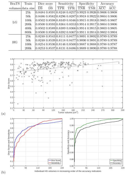
Table 1 presents the global performance indicators of the proposed segmen- tation procedure, average and overall values. The train data size does not have large impact on the segmentation accuracy: rising parameternF above 100k does not bring any benefit, neither for LG nor for HG glioma records. Average Dice scores obtained for LG data are slightly above 85%, while those for HG data are in the proximity of 82.5%. This difference can be justified by the quality of image data in the two data sets. However, the overall Dice scores are much closer to each other. The difference between average and overall sensitivity is only relevant in case of HG data. The average and overall values of specificity and correct decision rate (accuracy) hardly show any differences.
Figure 2 exhibits the Dice scores achieved for individual HG glioma volumes.
Figure 2(a) plots Dice scores against the size of the tumor (according to the ground truth). Each cross (×) represents the outcome of one MRI record. The dashed line indicates the linear trend identified by linear regression. The linear trend indicates that accuracy if better for larger gliomas, but even for small ones the Dice score is almost 80%. Figure 2(b) plots the individual value of all four accuracy indicators obtained for HG data, in increasing order. These graphs clarify the distribution of these values and reveals that their median value is higher than the average. Similarly, Fig. 3 gives the same representations for the segmentation outcome of LG glioma records. The shape of the graphs are quite similar to the ones obtained for HG data. The biggest difference is in the linear trend against tumor size: Dice scores hardly change with the glioma size, but even small gliomas are segmented with high accuracy characterized by a Dice score over 85%. The accuracy indicator values presented in Figs. 2 and 3 were achieved with train data sizenF = 100k.
Specificity values around 99% are very important, as the number of negative pixels is very high. Lower values in specificity would mean the presence of a lot of false positives in the segmentation outcome. Correct decision rates are in the proximity of 98%, meaning that only one pixel out of fifty is misclassified.
Figure 4 shows some examples of segmented brains. One selected slice from six different HG volumes are presented, the four observed data channels, namely T1, T2, T1C and FLAIR, followed by the segmentation outcome drawn in colors.
Colors represent the following: true positives are drawn in green, false positives in blue, false negatives in red, and true negatives in gray. Mistaken pixels are either red or blue.
The proposed segmentation procedure was implemented in Python 3 pro- gramming language. The segmentation of a single MRI record, including all steps according to Fig. 1, requires approximately two minutes without using any parallel computation.
Table 1.Main global accuracy indicators
BraTS Train Dice score Sensitivity Specificity Accuracy volumes data size DS DSf TPR TPR] TNR TNR] ACC ACC]
LG
25k 0.8484 0.8591 0.8248 0.8257 0.9923 0.9926 0.9806 0.9808 50k 0.8486 0.8582 0.8296 0.8287 0.9918 0.9922 0.9804 0.9806 100k 0.8502 0.8598 0.8349 0.8346 0.9915 0.9918 0.9805 0.9807 200k 0.8500 0.8593 0.8364 0.8353 0.9914 0.9917 0.9804 0.9806 400k 0.8502 0.8589 0.8389 0.8366 0.9914 0.9915 0.9803 0.9805 800k 0.8500 0.8586 0.8392 0.8367 0.9911 0.9914 0.9802 0.9804 HG
25k 0.8248 0.8543 0.8111 0.8477 0.9891 0.9892 0.9789 0.9789 50k 0.8248 0.8539 0.8118 0.8477 0.9890 0.9891 0.9789 0.9789 100k 0.8254 0.8536 0.8146 0.8500 0.9887 0.9888 0.9788 0.9787 200k 0.8253 0.8537 0.8131 0.8486 0.9889 0.9890 0.9788 0.9788
(a) Tumor volume (cm3)
0 30 60 90 120 150 180 210 240 270 300 330
Dice Score
0.1 0.2 0.3 0.4 0.5 0.6 0.7 0.8 0.9 1.0
(b) Individual HG volumes in increasing order of the accuracy indicators
0 55 110 165 220
Dice Score and Sensitivity
0.0 0.1 0.2 0.3 0.4 0.5 0.6 0.7 0.8 0.9 1.0
Dice Score Sensitivity
0 55 110 165 220
Specificity and Accuracy
0.86 0.88 0.90 0.92 0.94 0.96 0.98 1.00
Specificity Accuracy
Fig. 2.Accuracy indicators obtained for individual HG records: (a) Dice scores plotted against the true size of the glioma; (b) Individual DS, TPR, TNR and ACC values plotted in increasing order.
(a) Tumor volume (cm3)
0 30 60 90 120 150 180 210 240 270
Dice Score
0.3 0.4 0.5 0.6 0.7 0.8 0.9 1.0
(b) Individual LG volumes in increasing order of the accuracy indicators
0 9 18 27 36 45 54
Dice Score and Sensitivity
0.2 0.3 0.4 0.5 0.6 0.7 0.8 0.9 1.0
Dice Score Sensitivity
0 9 18 27 36 45 54
Specificity and Accuracy
0.84 0.86 0.88 0.90 0.92 0.94 0.96 0.98 1.00
Specificity Accuracy
Fig. 3.Accuracy indicators obtained for individual LG records: (a) Dice scores plotted against the true size of the glioma; (b) Individual DS, TPR, TNR and ACC values plotted in increasing order.
Fig. 4.One slice from six different HG tumor volumes, the four observed data channels and the segmentation result. The first four columns present the T1, T2, T1C and FLAIR channel data of the chosen slices. The last column shows the segmented slice, representing true positives (|Γi(π)∩Λ(π)i |) in green, false negatives (|Γi(π)∩Λ(ν)i |) in red, false positives (|Γi(ν)∩Λ(π)i |) in blue, and true negatives (|Γi(ν)∩Λ(ν)i |) in gray, where iis the index of the current MRI record.
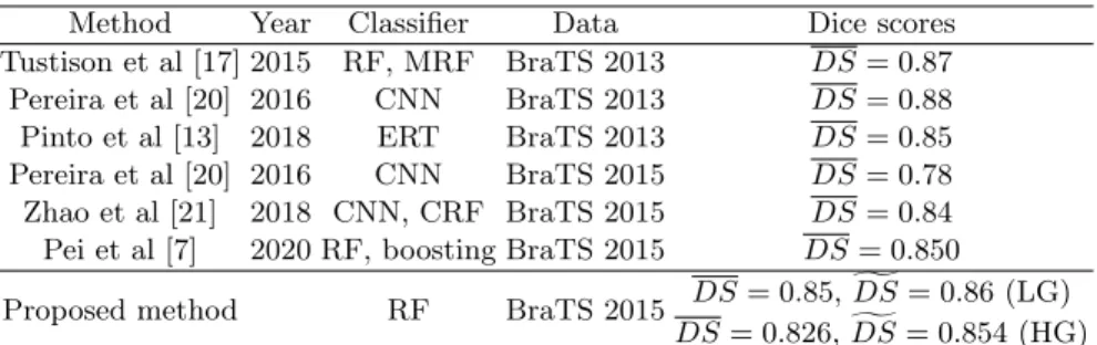
Table 2.Comparison with state-of-the-art methods
Method Year Classifier Data Dice scores
Tustison et al [17] 2015 RF, MRF BraTS 2013 DS= 0.87 Pereira et al [20] 2016 CNN BraTS 2013 DS= 0.88 Pinto et al [13] 2018 ERT BraTS 2013 DS= 0.85 Pereira et al [20] 2016 CNN BraTS 2015 DS= 0.78 Zhao et al [21] 2018 CNN, CRF BraTS 2015 DS= 0.84 Pei et al [7] 2020 RF, boosting BraTS 2015 DS= 0.850
Proposed method RF BraTS 2015 DS= 0.85,gDS= 0.86 (LG) DS= 0.826,gDS= 0.854 (HG) MRF - Markov random field, CRF - conditional random field
ERT - extremely randomized trees
4 Conclusions
This paper proposed a random forest based procedure for fully automatic seg- mentation of brain tumors from multi-spectral MRI data. The segmentation was accomplished in three main steps. Preprocessing was aimed at image data enhancement and feature generation. The random forest was trained to sep- arate normal pixels from positive ones, based on which it performed an initial classification of test pixels, providing them intermediary labels. Finally, the post- processing reevaluated the intermediary labels and produced regularized shapes to the detected tumors. The procedure was trained and evaluated using the BraTS 2015 train records. The achieved segmentation accuracy is characterized by an overall Dice score between 85-86%, both in case of LG and HG glioma records, which is competitive with respect to state-of-the-art methods, as indi- cated in Table 2.
References
1. Mohan, G., Subashini, M. M.: MRI based medical image analysis: Survey on brain tumor grade classification. Biomed. Sign. Proc. Contr.39, 139–161 (2018) 2. Menze, B. H., Jakab, A., Bauer, S., Kalpathy-Cramer, J., Farahani, K., Kirby,
J., et al.: The multimodal brain tumor image segmentation benchmark (BRATS).
IEEE Trans. Med. Imag.34, 1993–2024 (2015)
3. Bakas, S., Reyes, M., Jakab, A., Bauer, S., Rempfler, M., Crimi, A., et al.: Identi- fying the best machine learning algorithms for brain tumor segmentation, progres- sion assessment, and overall survival prediction in the BRATS challenge. arXiv:
1181.02629v3, 23 Apr 2019.
4. Gordillo, N., Montseny, E., Sobrevilla, P.: State of the art survey on MRI brain tumor segmentation. Magn. Res. Imag.31, 1426–1438 (2013)
5. Njeh, I., Sallemi, L., Ben Ayed, I., Chtourou, K., Lehericy, S., Galanaud, D., Ben Hamida, A.: 3D multimodal MRI brain glioma tumor and edema segmentation: a graph cut distribution matching approach. Comput. Med. Imag. Graph.40, 108–
119 (2015)
6. Rehman, Z. U., Naqvi, S. S., Khan, T. M., Khan, M. A., Bashir, T.: Fully auto- mated multi-parametric brain tumour segmentation using superpixel based classi- fication. Expert Syst. Appl.118, 598–613 (2019)
7. Pei, L. M., Bakas, S., Vossough, A., Reza, S. M. S., Murala, C., Iftekharuddin, K. M.: Longitudinal brain tumor segmentation prediction in MRI using feature and label fusion. Biomed. Sign. Proc. Contr.55, 101648 (2020)
8. Tong, J. J., Zhao, Y. J., Zhang, P., Chen, L. Y., Jiang, L. R.: MRI brain tumor segmentation based on texture features and kernel sparse coding. Biomed. Sign.
Proc. Contr.47, 387–392 (2019)
9. Menze, B. H., van Leemput, K., Lashkari, D., Riklin-Raviv, T., Geremia, E., Al- berts, E., et al: A generative probabilistic model and discriminative extensions for brain lesion segmentation – with application to tumor and stroke. IEEE Trans.
Med. Imag.35, 933–946 (2016)
10. Szil´agyi, L., Lefkovits, L., Beny´o, B.: Automatic brain tumor segmentation in mul- tispectral MRI volumes using a fuzzyc-means cascade algorithm. In: Proc. 12th International Conference on Fuzzy Systems and Knowledge Discovery, pp. 285–291.
IEEE (2015)
11. Li, Q. N., Gao, Z. F., Wang, Q. Y., Xia, J., Zhang, H. Y., Zhang, H. L., Liu, H. F., Li, S.: Glioma segmentation with a unified algorithm in multimodal MRI images.
IEEE Access6, 9543–9553 (2018)
12. Islam, A., Reza, S. M. S., Iftekharuddin, K. M.: Multifractal texture estimation for detection and segmentation of brain tumors. IEEE Trans. Biomed. Eng. 60, 3204–3215 (2013)
13. Pinto, A., Pereira, S., Rasteiro, D., Silva, C. A.: Hierarchical brain tumour seg- mentation using extremely randomized trees. Patt. Recogn.82, 105–117 (2018) 14. Imtiaz, T., Rifat, S., Fattah, S. A., Wahid, K. A.: Automated brain tumor seg-
mentation based on multi-planar superpixel level features extracted from 3D MR images. IEEE Access8, 25335–25349 (2020)
15. Lefkovits, L., Lefkovits, S., Szil´agyi, L.: Brain tumor segmentation with optimized random forest. In: Crimi, A., Menze, B., Maier, O., Reyes, M., Winzeck, S., Han- dels, H. (eds.) Brainlesion: Glioma, Multiple Sclerosis, Stroke and Traumatic Brain Injuries. LNCS, vol. 10154, pp. 88–99. Springer, Cham (2017)
16. Lefkovits, S., Szil´agyi, L., Lefkovits, L.: Brain tumor segmentation and survival prediction using a cascade of random forests. In: Crimi, A., Bakas, S., Kuijf, H., Keyvan, F., Reyes, M., van Walsum, T. (eds.) Brainlesion: Glioma, Multiple Sclero- sis, Stroke and Traumatic Brain Injuries. LNCS, vol. 11384, pp. 334–345. Springer, Cham (2019)
17. Tustison, N. J., Shrinidhi, K. L., Wintermark, M., Durst, C. R., Kandel, B. M., Gee, J. C., Grossman, M. C., Avants, B. B.: Optimal symmetric multimodal tem- plates and concatenated random forests for supervised brain tumor segmentation (simplified) with ANTsR. Neuroinform.13, 209–225 (2015)
18. Zhang, N., Ruan, S., Lebonvallet, S., Liao, Q., Zhou, Y.: Kernel feature selection to fuse multi-spectral MRI images for brain tumor segmentation. Comput. Vis.
Image Understand.115, 256–269 (2011)
19. Sert, E., Avci, D.: Brain tumor segmentation using neutrosophic expert maximum fuzzy-sure entropy and other approaches. Biomed. Sign. Proc. Contr.47, 276–287 (2019)
20. Pereira, S., Pinto, A., Alves, V., Silva, C.A.: Brain tumor segmentation using convolutional neural networks in MRI images. IEEE Trans. Med. Imag.35, 1240–
1251 (2016)
21. Zhao, X. M., Wu, Y. H., Song, G. D., Li, Z. Y., Zhang, Y. Z., Fan, Y.: A deep learning model integrating FCNNs and CRFs for brain tumor segmentation. Med.
Image Anal.43, 98–111 (2018)
22. Nema, S., Dudhane, A., Murala, S., Naidu, S.: RescueNet: An unpaired GAN for brain tumor segmentation. Biomed. Sign. Proc. Contr.55, 101641 (2020) 23. Lˆe, M., Delingette, H., Kalpathy-Cramer, J., Gerstner, E. R., Batchelor, T., Unkel-
bach, J., Ayache, N.: Personalized radiotherapy planning based on a computational tumor growth model. IEEE Trans. Med. Imag.36, 815–825 (2017)
24. Vovk, U., Pernu˘s, F., Likar, B.: A review of methods for correction of intensity inhomogeneity in MRI. IEEE Trans. Med. Imag.26, 405–421 (2007)
25. Szil´agyi, S. M., Szil´agyi, L., Icl˘anzan, D., D´avid, L., Frigy, A., Beny´o, Z: Intensity inhomogeneity correction and segmentation of magnetic resonance images using a multi-stage fuzzy clustering approach. Neur. Netw. World09(5), 513–528 (2009) 26. Szil´agyi, L., Szil´agyi, S. M., Beny´o, B.: Efficient inhomogeneity compensation using
fuzzyc-means clustering models. Comput. Meth. Progr. Biomed108, 80–89 (2012) 27. Tustison, N. J., Avants, B. B., Cook, P. A., Zheng, Y. J., Egan, A., Yushkevich, P. A., Gee, J. C.: N4ITK: improved N3 bias correction. IEEE Trans. Med. Imag.
29, 1310–1320 (2010)
28. Szil´agyi, L., Icl˘anzan, D., Kap´as, Z., Szab´o, Z., Gy˝orfi, ´A., Lefkovits, L.: Low and high grade glioma segmentation in multispectral brain MRI data. Acta Univ.
Sapientia, Informatica10(1), 110–132 (2018)