Coordinated dense aerial traffic with self-driving drones
Boldizs´ar Bal´azs1 and G´abor V´as´arhelyi1,2
Abstract— In this paper we present a general, decentralized air traffic control solution using autonomous drones. We chal- lenge some of the most difficult dense traffic situations, namely, crosswalk and package-delivery scenarios, where intelligent collective collision avoidance and motion planning is essential for a jam-free optimal traffic flow. We build up a force- based distributed multi-robot control model using a tunable selection of interaction terms: anisotropic repulsion, behaviour- driven velocity alignment, self-organized queueing and conflict- avoiding self-driving. We optimize the model with evolution in a realistic simulation framework and demonstrate its applicability with 30 autonomous drones in a coordinated outdoor flight within a densely packed virtual arena.
I. INTRODUCTION
UAVs in common airspace are already challenging current centralized traffic-organizing schemes while their number is expected to explode in this decade. To assist or even replace human airspace control efforts, hybrid and fully decentralized aerial traffic solutions will become a key in the near future.
To facilitate this trend, we show a self-organizing solution to control large numbers of autonomous drones with individual flight tasks. We use an agent-based algorithm that has been inspired by recent, custom-tailored variants of the original Vicsek-model [1], but also contains optimized traffic-specific interaction terms. The local nature of this approach promises the scalability of the solution to even global scale.
There is already vast literature on optimizing ground traffic, which is restricted in most cases to quasi-one- dimensional roads. This boundary condition together with human imperfection in concentration, reaction time and limited sight cause jams, slow traffic and also many accidents [2]–[4]. There is an ongoing revolution to wipe out these inevitable human faults by autonomous cars [5]–[7].
The complexity of two- or three-dimensional aerial traffic with ever-growing number of agents can go beyond that of ground traffic [8], even though the only infrastructure needed, air, is present everywhere and in general there is a lot more space in three dimensions than on one dimensional roads.
At the same time, aerial traffic might also be constrained by virtual roads and restricted air spaces, close-to-ground air traffic has to handle obstacles in 3D, while motion and communication in the air is always much more challenging than on the ground [9]. Centralized path-planning - e.g. game theory based [10] or bioinspired [11] - calculates close to optimal routes for a couple of agents, but the scalability of
1ELTE Department of Biological Physics, Budapest, Hungary, bboldizsar@hal.elte.hu
2MTA-ELTE Statistical and Biological Physics Research Group, Bu- dapest, Hungary, vasarhelyi@hal.elte.hu
such approaches is questionable due to central communica- tion and computational complexity. Self-organization is an excellent direction to address all these difficulties [12], [13].
This approach is used by biological systems [14], [15], and technological innovations [16], [17], too.
The first step of multi-drone coordination was to achieve synchronized flight of a flock of drones as a common task for all agents [18]–[21]. As a second step, here we intent to organize the traffic flow of a flock of drones, where coordination is still needed but the flight mission of each agent is independent and thus there are a lot more conflicts in the air to be resolved on the spot. Moreover, we investigate the most difficult traffic scenarios of densely packed aerial drones. We forge situations where the drones are compelled to use every bit of the available airspace if they want to reach their targets quickly. Additionally, the traffic flow is demanded to be collision- and oscillation-free. All of these self-organized global features need to emerge from individual behaviour based on limited local information. Our model runs in two dimensions to harden the task by limiting possible movement directions to the horizontal plane, but it can be used to handle full 3D traffic as well, if needed.
To perform optimal drone traffic, we build upon our previ- ously proposed force-based simulation model of UAV traffic [22] but will highly exceed it in the basic concepts about the role of the interactions and the generality of the solutions even in situations where our previous model failed (e.g., avoiding traffic jams around common targets). Furthermore we will also demonstrate the functionality of our model with actual field experiments using 30 fully autonomous drones.
First, in the next section we will give a detailed intro- duction to our agent-based algorithm that is executed on all drones in a distributed way.
II. TRAFFIC MODEL
We build up our control algorithm from four unique interaction terms. First we will give a descriptive explanation of each term which will be followed by exact mathematical equations.
The motivation for the four major interactions in our model can be viewed as steps from rudimentary to complex behaviour. Repulsion and alignment are fundamental terms of coordination used in the majority of flocking models [1], [19], [23]. Repulsion is in charge of avoiding collisions, while alignment aims to synchronize motion and thus in general to diminish oscillations. Additionally, we use self- drivingto make the agents move circumspectly around each others and prevent collision conflicts, and self-organized 2018 IEEE International Conference on Robotics and Automation (ICRA)
May 21-25, 2018, Brisbane, Australia
queueingbehaviour, which is already halfway between local and global problem-solving, as agents share information about the global target of their local neighbours in the queue.
The joint usage of these interactions disrupts this simple hierarchical picture. It turns out in real flights that agent- agent interactions cannot be driven by repulsion, as it ends up in oscillations if the alignment is small enough to let anything happen in the sky. Therefore, we need an agile self- driving term to keep the agents away from collision-course first. Such a well designed conflict-prevention term liberates the repulsion term from its last resort role, so it may become anisotropic to make the agents slip through frequented areas quicker. The smooth flow provided by these terms allow the agents to reduce the number of neighbours to align their velocity to, with behaviour-driven selective friction. As the agents handle well their neighbours moving in any direction, an additional queueing term can be introduced to wait for each other patiently at a common target, minimizing the blocking effect of other queuers.
In our momentary force-based model the ith agent (with positionriand velocityvi) calculates its momentary desired velocity according to the interaction terms described above:
˜
vi=vrepi +valigni +vtargeti . (1) In the followings we give a proper mathematical definition to all of these interaction terms.
A. Anisotropic repulsion
Isotropic repulsion is generally used in flocking algorithms to avoid agents getting too close to each other. If they move into the same direction during flocking, repulsion sets the average inter-agent distance. But if they move in the opposite direction during a traffic situation, repulsion pushes agents away from their desired direction, creating oscillations.
In our anisotropic repulsion term we distinguish agents based on the difference between their direction of motion.
If thejth agent is close to theith agent, but their direction of velocity is the same (with an angular threshold of ±π3), then it is not the same type of threat as if they go into the opposite direction. In the latter case, it is better to evade each other than to oscillate. In fact, in jam situations it also seems favourable to form some kind of chain of the agents going in the same direction.
Both of these reasonable goals can be achieved by intro- ducing anisotropy (A) into the repulsion:
virep=X
j6=i
urepij vijrep, (2) where the double indices refer to the interaction between the ith and jth agents, from the viewpoint of agent i. The magnitude of repulsionvijrepis calculated by the function
vrepij (rij) =
(prep(R0−rij) rij < R0
0 rij ≥R0, (3)
whereprepis a linear gain,R0is the radius of the repulsive zone and rij = |rij| = |rj −ri|. The repulsion direction
ϕ
ρ
isotropic anisotropic
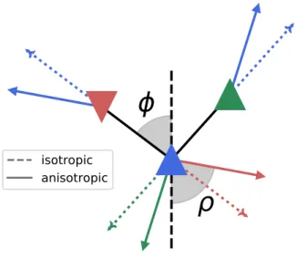
Fig. 1. Explanation of the anisotropic repulsion. Agents are depicted with colored triangles pointing towards their direction of motion. The anisotropic response between the blue and green agents (↑↑, Eq. (6)) is different from the response between the blue and red agents (↑↓, Eq. (7)). Dashed vectors show the isotropic repulsion of agents as a response to neighbours with given colors. The sum of these responses would force the agents to move backwards. This is a suboptimal choice, as the green agent is about to open up free space at the right side of the blue one. The sum of the anisotropic responses represented by the solid vectors exploits the situation and forces the blue agent to fill in the space opened up by the green agent. The effect of the blue agent on its neighbours is also advantageous. It forces the red agent to evade the blue one more and lets the green one continue its route towards its target with less interference. The input (φ) and output (ρ) angles of Eq. (5) are shown for the blue agent with respect to the red one.
urepij is the only direction which satisfies (rit×rij)· urepij ×rit
>0 (4) whererit=rtargeti −ri and
ρ=
(h↑↑(φ) α(rit,vj)≤π3
h↑↓(φ) α(rit,vj)>π3, (5) whereα(., .)is the angle between two input vectors,ρ= α urepij ,−rit
andφ=α(rij,rit).
Eq. (4) and (5) mean that urepij lies on the opposite side of −rit than rij and is making ρ angle with it, as seen in Fig. 1.
The shape of theh↑↑(.)andh↑↓(.)functions is determined by the anisotropy parameterA. If anisotropy is0, we get the isotropic repulsion with urepij = rrji
ji ≡ N(rji). This means that both h(.) functions are linear with a slope of 1. As A increases towards its limit 1, the two functions deviate from this single linear shape to piecewise linear functions, with the boundary conditionh↑↑(π) =h↑↓(π) =π:
h↑↑(φ) =
(A·φ φ≤π2
π+A·(φ−π) φ >π2 (6) h↑↓(φ) =
1−A
2
(φ−π) +π. (7)
In Eq. (6) theA·πjump at π2 magnifies the lane-forming phenomenon, what is already present in similar systems at equilibrium [14], but we want to accelerate its construction to increase the flow. Similarly, the deviation from the identity function in h↑↓(.) results in the acceleration of evading provided also by the self-driving term, as can be seen later.
B. Selective alignment
If the goal of the fleet is not to flock together coherently, alignment may seem superfluous. Indeed, it turns out to be useful in any stochastic collective flight to reduce oscillations and to prevent dangerous situations by eliminating too high velocity differences between close-by neighbors. In other words, while repulsion is a form of excitation, alignment acts as a useful damping term. Our alignment term is
valigni = X
j∈Ai
N(vji)·
·θ vji−max valign, D rij, Ralign, palign, aalign , (8) whereθis the Heaviside step function, andDis a smooth and optimal braking curve to decay velocity as a function of distance, with explicitly taking into account the motion constraint of finite acceleration capabilities:
D(r, d, p, a) =
0 r < d
p(r−d) d < r < d+pa2
q
2a(r−d)−ap22 d+pa2 < r,
(9)
whereais the acceleration limit,pis a linear gain in the v-r plane anddis a distance offset forD(.)in the v-r plane.
The square root part corresponds to a constant deceleration.
The reason one needs to cut it - continuously to first order - with a linear part is that a little noise in distance can cause enormous difference in output velocity near the point of infinite derivative.
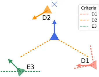
To reduce undesired alignment, every agent may select the neighbours it aligns to. To decide whether alignment should be used for a neighbour (i.e., it is part of the setAi), the agent first checks three conditions. The first two represent possible danger: D1) the neighbour comes towards the agent (with fixed angular threshold±π4); D2) the neighbour is between the agent and its target (with fixed angular threshold ±2π3 relative to the agent-target direction). The third condition is related to efficiency: E3) the velocity of the neighbour points towards the target of the agent (with fixed angular threshold
±π2), i.e., they both head to similar directions in a flock.
If at least two of these three conditions are valid, we use alignment. Otherwise, we switch it off as the situation is safe enough and would not be efficient enough with alignment.
Fig (2) visualizes all conditions when alignment can be neglected.
C. Agile self-drive
Every agent moves towards its target withvitarget. In open space this vector has a magnitude of vSPP, a predefined travelling speed. However, if there is any neighbour in the
E3 D1
D2
Criteria D1 D2 E3
Fig. 2. Selectivity of alignment. Neighbors of the blue agent show three cases when alignment can be switched off as each of them holds only one danger or efficiency criteria and thus motion remains safe and becomes more efficient without alignment. These three conditions are: D1) coming towards the agent; D2) being in front of the agent; E3) moving towards the target of the agent. For sake of simplicity the blue agent moves exactly towards its target. Auxiliary lines represent angular thresholds of the one and only held criterion for each neighbor.
way, it needs to be shrunk and/or rotated to prevent getting into the range of repulsion.
The agent reduces its target velocity iteratively. It chooses its closest neighbour which is inside the rectangle with length of the distance of the previously chosen neighbour (or the target at the start of the iteration) and half-width of a safety distance RS, pointing in the direction of vtarget. The agent separates the component of vtarget pointing towards the chosen neighbour and reduces it according to D(rij, RS, ptarget, atarget). This reduced component is rotated with an angle of T ·sin−1(RS/rij) towards the direction of vtargeti . The tangentiality parameter T defines the amount of rotation. At T = 1 the remaining part gets rotated exactly to the tangent line, while T = 0 switches off rotation completely. The rotated component is added back to the perpendicular component. The final magnitude is constrained not to grow in any step. Since the agent chooses closer and closer neighbours in every step and the velocity magnitude decreases, the iteration is guaranteed to stop either at the closest neighbour or at zerovitarget. Fig. 3 summarizes the algorithm behind the self-drive mechanism.
D. Radial queueing
When approaching a target it is reasonable to require that the agent decreases the magnitude of vtargeti smoothly as getting closer. We do this with the previously introducedD(.) function. To keep the number of parameters manageable, this term uses the same values for acceleration and slope as the self-driving term (as these are similar cases of deceleration, in front of a target or another agent). If there are more agents approaching the same target, they queue up and thus might have to stop before they reach their target. To calculate the
before after RS
Fig. 3. Agile self-driving with T = 1. The green neighbour is out of the danger zone (blue rectangle), hence does not force the blue agent to decrease its original target velocity represented by a solid blue vector.
TheRS(black ruler) safety environment of the red neighbour would be intersected though, so the agent decomposes its target velocity into a component pointing towards the neighbour and an orthogonal component, both represented by blue dashed vectors. The former component gets decreased according to the function described in Eq. (9) with the parameters that can be found in Table I. Having decreased the component it gets also rotated to the tangential direction (red dashed vector), and is added back to the orthogonal component. The result isvtarget, represented by the solid red vector. If there were more neighbours closer than the red one, more iterations would be needed to get the final target velocity vector.
individual stopping point, agents search for the neighbour who is i) closer to the agent than a queueing interaction range RQR; ii) going towards the same target or within a safety radius ofRS; iii) closer to the target than the agent itself and iv) furthest away from the target among agents fulfilling i-iii.
If this neighbor exists, this will be the one in front of the agent in the queue, called the q-agent. In this case, the agent stops at a queueing distanceRQ further from the target than the q-agent. If the q-agent does not exist, the agent wants to slow down to zero exactly at the target.
This interaction forces the agents not to approach their targets, but to wait patiently in a queue instead. The queue is virtual, the agents do not form lines in real space. Queueing can be treated as a very useful collective behavioural state of the agents (as a form of instantaneous, self-organized order hierarchy) to avoid unnecessary self-excitation in the repulsive range in certain situations. This term helps to prevent giant over-packed jams around a frequented target, where even the agent who has reached its goal and wants to move to another one can not move due to the dense packing.
However, the model also needs to take care of situations, when despite their ability to move freely towards their target, multiple agents freeze because a few agents closer to the target are stuck in a jam. The following method rules out these situations: 1. check if the agent who is closer to the target of q-agent than the q-agent itself and is the closest neighbour of the q-agent is going to the same target as q- agent. 2. If it is going elsewhere, and it is closer to q-agent thanR0, then we do not queue up behind q-agent, since he is stuck in a jam independent of our queueing.
As a result of numerous simulation, RQR defines the queueing behaviour more intensively thanRQ, so the latter will be ruled out from the free parameters, with the following
estimation. Thenagents closest to the common target all take each other into account if the furthest isRQR/2 away from the target. This implies that the nth agent is nRQ away.
All the n agents need free space with radius RS around themselves, so(nRQ)2'nR2S. From all this we get
RS = r
RQ
RQR
2 , (10)
thusRQ can be defined by free parametersRQR andRS. There is one last possible situation when the agent has to stop before its target: when a neighbour is behind the target, but its security zone of radiusRS intersects with the line segment between the agent and the target. This shall be resolved by stopping at this intersection.
E. Model summary
In this section we introduced a traffic model that generates a desired velocity as a sum of three velocity terms provided by the specific interactions, as it can be seen in Eq. (1).
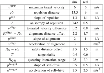
This velocity depends on the world agents observe around themselves (set ofrjs andvjs) and the actual values of the free model parameters, which are summarized in Table I.
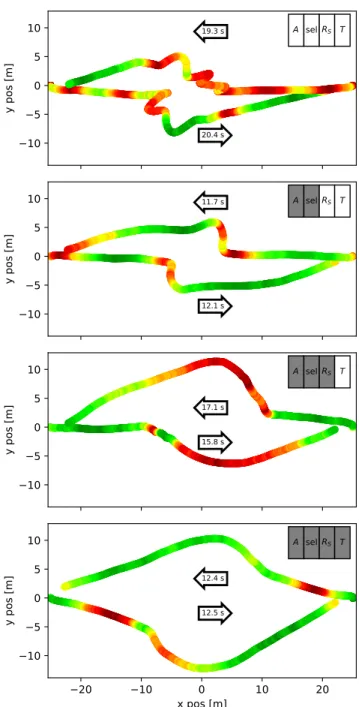
In the beginning of this section the origin and nature of the terms was introduced. After having rigorously explained the exact functioning of the terms, Fig. 4 gives a general overview of the new features through two-agent interactions.
As one can see on the first subfigure, isotropic repulsion with a constant target velocity leads to oscillating and ineffective motion and unselective alignment holds off the agents from leaving the impact zone even after passing by each other.
Anisotropy and selectivity offers a quick resolution of the two-agent conflict (second subfigure), but resulting trajec- tories are still not smooth enough. Changing the constant target velocity to the one given by the self-driving term (third subfigure) smoothens out the trajectory a bit, but with the compromise of much slower motion. Making the self-drive agile (fourth subfigure) further enhances the smoothness of the curves, improves the performance while maintains mutual avoidance. In the final solution distance between agents is increased, which increases safety but creates longer paths. However, speed is maximal most of the time which compensates for the loss of efficiency.
In the next section we tune the free parameters with realistic simulations to obtain an optimal working model to be used on real drones as well.
III. REALISTIC SIMULATION
Our simulation framework imitates realistic conditions by providing the agent imperfect information about its neigh- bours and its sensors due to limited communication range, non-zero communication time delay tdelay and noise. The simulation also limits the velocity of agents to reach the desired value defined in Eq. (1) with finite accelerationamax. All details about the used realistic conditions can be found in our previous work [24].
To investigate how the four new features of agile self- drive, anisotropic repulsion, selective friction and radial
A selRS T
−10
−5 0 5 10
y pos [m]
20.4 s 19.3 s
A selRS T
−10
−5 0 5 10
y pos [m]
12.1 s 11.7 s
A selRS T
−10
−5 0 5 10
y pos [m] 15.8 s
17.1 s
A selRS T
−20 −10 0 10 20
x pos [m]
−10
−5 0 5 10
y pos [m] 12.5 s
12.4 s
Fig. 4. Effect of the interaction terms demonstrated by simulating two agents in a direct conflict. Coloring of the trajectories is mapped to the velocity (red-slow, green-fast, with the same color map as in Fig.
7). Turning on the features of the interactions (A: 0→0.42, sel: off→on, RS: 0 m→16 m,T: 0→1) is symbolized by gray background in the upper right corner. Other parameters are set according to Table I. Arrows show the direction of motion and the time needed for the agent to reach its target.
The right-hand rule bias isnot included in the ruleset, we chose similar situations for better comparability.
queueing handles hard situations, we set the mean free path, l = L/√
N as low as 20 −30m, while maintaining a vSPP = 6m/s target velocity. Note that the lower limit is hardly 2vSPP tdelay+vSPPa−1max/2
, what is the distance where two frontally moving agent can stop with late reaction and limited deceleration. Moreover, we forge two target scenarios demonstrating the two most challenging aspects
of traffic: i) multiple path conflicts; ii) flow bottlenecks.
In the first scenario drones are placed in a ’crosswalk’
situation: half of agents start from one side of the arena, while the rest from the opposite side. Every time an agent gets to its target it takes a new target randomly selected on the opposite edge of the arena. Initially this results with two fronts of agents colliding into each other (same as with people on green light on a crosswalk [25]) and later several agents meeting near the center with a potential head- on collision. These path conflicts form a testbed for the anisotropic repulsion and the self-driving term, as the agents have to evade each other effectively, and form lanes to open up space for the rest. Increasing the number of agents, while keeping the mean free path constant makes the targets more dense on the one-dimensional arena-edge, so queueing also plays a more and more important role.
In the second ’star’ scenario all of the agents have one common destination: the center of the square-formed, L- sized arena. Having reached this destination they head to a randomly selected point on the edge of the arena. This bot- tleneck situation is a perfect testbed for the radial queueing behaviour (and could be of interest e.g. for drone package delivery applications where a central post office has to be reached by all agents).
For the optimization of a wide range of parameters we used the state-of-the-art evolutionary optimizing tool CMA-ES [26]. To quantitatively decide if one parameter set is better than the other, one needs to define a fitness function.
Our goal is to make the agents reach the most possible targets in 600 seconds, without colliding into each other, and without burning energy for unnecessary accelerations.
For sake of simplicity each term got transformed into [0,1].
These requirements result in a fitness function that was also used in [22], expanded by a third, acceleration minimizing term.
F = C2
(< ψcoll>t+C)2
< veff >t
vSPP
amax−<|a|>t
amax
, (11) where ψcoll is the collision risk, i.e., the normalized probability of two agents being closer to each other than 5 m, as defined in [22],C=2E-6, veffi is the effective velocity of agentidefined as the velocity component in the direction of the ideal waypoint vector pointing from the last to the next target,ai is the acceleration of agenti,amax= 6m/s2 is the acceleration limit of the simulated agents, < . >t
denotes averaging through all time instances (t) andxis the average of x for all agents. Evolutionary optimization for 100 agents and L = 250m ran with 100 generations and 100 phenotypes per generation on a computer cluster. The optimization works on a superagent level, as all the fleet uses the same parameters in one simulation, and the evolution searches for the best average fitness for the fleet. The results represent parameter sets that produce a safe and effective traffic flow. Gladly enough this was almost the same for both target scenarios concerning the most dominant parameters:
R0 ' 10m, RQR ' 25m, RS−R0'1m, T ' 0.7, A'0.5.
TABLE I MODEL PARAMETERS
sim. real
vSPP maximum target velocity 6 6 m/s
R0 repulsion distance 13.5 9 m
prep slope of repulsion 1.3 1.1 1/s
A anisotropy of repulsion 0.42 0.5 valign tolerated velocity difference 0.2 0.8 m/s Ralign−R0 alignment distance offset 2.2 1.7 m
palign slope of alignment 2 1 1/s
aalign acceleration of alignment 3 3 m/s2 RS−R0 safety distance offset 2.5 1.5 m
T tangentiality 0.4 0.6
RQR queueing interaction range 35 30 m
ptarget slope of self-drive 0.5 0.5 1/s
atarget acceleration of self-drive 2.5 2.5 m/s2
Evolution provided us optimal values and working ranges of parameters where fitness was found to be high. Starting from these values we selected final parameters for the actual system size used in real experiments (N = 30, L = 150m) through visual inspection of the simulations. Note that final fine tuning of the system is hardly avoidable due to the obvious limitations of a quantifiable fitness function in capturing the overall quality (e.g. ’smoothness’ in our case) of a complex system (cf. definition of IQ for human
’intelligence’ [27]). In other words, two different parameter sets may give the same value for collision risk, effective velocity, acceleration or other simple descriptors, but the overall difference in quality could still be perceptible.
The main difference between the evolutionary optimum and the final parameter setup was in the role of the repulsion.
Evolution utilized repulsion for collision avoidance but in the real system we wanted to avoid repulsion-driven oscillations completely so we decreased the range of repulsion and the anisotropy and increased the safety distance of self- drive instead as a preventive, conservative action, with the compromise of some fitness loss.
To minimize the uncertainty in the parameter choice we also swept around all the final parameters and based on 5 simulations at each parameter value we chose the most effective version for the real flight system size. Switching between the human pattern-recognition and the data-driven computer analysis is called the centaur method, and has been successfully applied in medical challenges [28], [29]. The concluded parameter sets were so close for the two target scenarios that we kept the set of the more difficult crosswalk scenario. The final parameters can be seen in Table I.
As a final check in simulation, we created statistics of the effective velocity (veff), the overall magnitude of the traffic flow, i.e., the flux (veff/l) and the collision risk (Ψcoll) as a function of the mean free path (l) in the crosswalk scenario with 100 agents. Results give a typical density dependence, with low collision risk and relatively high effective velocity even in the dense traffic range, with a maximal flux at
0 25 50 75 100 125 150 175 200
Mean Free Path √L2/N (m) 0
1 2 3 4 5 6
Effective Velocity (m/s)
max=0.096/s @ 36m
vSPP flux collision risk veff
0.00 0.05 0.10 0.15 0.20 0.25 0.30 0.35 0.40
Average Collision Risk (*1e-6)
Fig. 5. Traffic flow statistics as a function of mean free path (density).
Twenty 10-minute simulations were averaged at each measurement point.
Standard deviations are shown with error bars, but they are too small for the flux and the mean free path to be visible. The overall flux has a maximum at 36 m mean free path, which is a relatively dense traffic situation.
around l = 36 m (see Fig. 5). The collision risk got a tenfold decrease compared to that of [22], while keeping the maximal flux practically the same. Note that the crosswalk scenario leads to more dangerous head-on situations than others studied in the previous paper. Additionally, the proper handling of the finite acceleration capabilities enables our model to work withvSPP= 6 m/s. This leads to a 1.5 times increase of the flux in the low-density regime.
To assess the star scenario we calculated the time between two agents reaching the central target in the queue. The statistical average of 20 simulations for each of the 48 mean free path values between 22 and 365 m is mostly independent of density (viz. reaching the central point is a bottleneck) with an overall value within 12±1 s. The number of collisions was zero in every simulation. Visualizations of both scenarios can be seen in theSupplementary Video.
IV. REAL FLIGHTS
Real experiments were performed with our tailor-made quadcopter fleet, designed for swarming missions. The drones are based on a PixHawk low-level autopilot [30], running a custom modified version of the ArduCopter code [31]. Positioning is based on GNSS, which required an open air outdoor space. The low level autopilot receives desired velocity commands at 20Hz rate from an Odroid minicomputer. This high-level autopilot executes our traffic algorithm, using information received from other fleet mem- bers through an ad-hoc wireless network in the form of UDP packages. Communication between drones and computation of the actual control signals remained local and distributed at all times.
The final experiment with the 30-drone fleet took place on a windless, sunny day around Paty, Hungary. Having tested the parameter set before for 6 drones and both scenarios,
we went for 10 and 20 drones first. Note that the simula- tion framework provides solutions for worst-case scenarios regarding noise and delay to make sure the uncertainty in the reality gap will not decrease safety. The first real tests happened to show stable enough behaviour to further optimize some parameters and maximize the flow. The final parameter values used for experiments are summarized in Table I. The final experiment had 30 agents, moving in a 150×150m arena with 6 m/s according to the more difficult crosswalk target scenario.
Note that the takeoff position of the drones had some effect on initial transient performance. While the algorithm is prepared to prevent risky situations, neither of anisotropic repulsion, selective friction, agile self-drive and radial queue- ing is purely optimized or even dedicated to handle situations starting from risk already. Consequently, when the drones were not spread out initially as in the simulation but took off very close to each other (e.g., with 5-7 m spacing), the initial movement of the drones was somewhat erratic as they started from within the range of anisotropic repulsion, which pushed them away from each other at high speed. It is not an actual fault, because this is a situation what the algorithm would never allow to happen. Nonetheless this is a field, where there is space for improvement, e.g., by introducing a new behavioural phase to handle such ”panic”
situations effectively. Anyhow, after the initial transient, the fleet always found a formation where every drone had its own safe space, and from that point on, they reached their targets fast and smoothly while using the available space smartly.
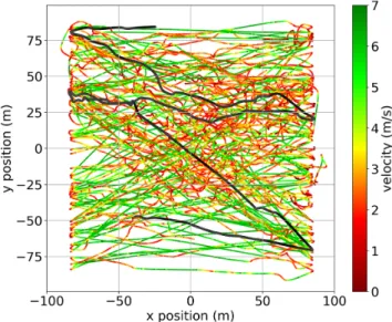
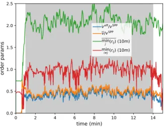
Fig. 6 contains a long exposure photo of the experiment, Fig. 7 shows plotted trajectories of the drones in the horizon- tal plane, Fig. 8 shows order parameters of the flight collected from flight logs and the Supplementary Video shows raw footage and visualization of the flight with 30 drones. All visualizations demonstrate the smooth, stable and efficient functioning of the algorithm in a real outdoor experiment.
V. DISCUSSION
In this paper we presented an agent-based, decentralized and scalable solution for difficult 2D air traffic situations.
We proposed four new interaction terms: repulsion became anisotropic and alignment became selective to adapt more to traffic situations, while queueing and self-drive got in- troduced to resolve oscillations and jams. Eliminating these problems enabled our UAV fleet of 30 drones to complete random missions of coordinated flight with conflicting tasks in dense environments.
Keeping the mean free path constant, the same set of parameters proved to be a fine real-life solution for several systems sizes of 6, 10, 20 and 30 agents. Moreover, our parameter set keeps on working well in simulation with significantly increased (up to 12 m/s) speed. These two facts represent a very promising feedback on our approach for handling difficult traffic situations.
Further improvement in this field can be obtained by also handling arbitrary obstacles in the way or introducing heterogeneity/hierarchy among agents.
Fig. 6. Long exposure photo of a flight with many drones during a 2D traffic experiment at 20 m altitude. The color of the drones changed according to their behavioural state: green means that there are no obstacles in the way, blue/purple means that the drone needs to break and avoid others, while red means that the drone is in a queueing phase.
Fig. 7. Five minutes of horizontal trajectories from a flight with 30 drones. Colour of the trajectories is mapped to horizontal velocity. Curvy red sections represent collision avoidance and evasion, occurring mostly in the middle of the arena, while straight green lines represent free motion towards the targets arranged in two sides of the arena. One trajectory is shown in grey to highlight individual motion. The trajectories show smooth deceleration and collision avoidance behaviour without uncoordinated oscillations and demonstrate the efficiency of the algorithm (seeSupplementary Videofor a dynamic visualization of the flight).
ACKNOWLEDGMENT
This work was partly supported by the following grants:
USAF Grant No: FA9550-17-1-0037; K 16 Research Grant
0 2 4 6 8 10 12 14 time (min)
0.0 0.5 1.0 1.5 2.0 2.5
order params
veff/vSPP v/vSPP minj (rij) (10m) mini≠j(rij) (10m)
Fig. 8. Order parameters as a function of time during a 15-minute flight with 30 drones.veff/vSPPis the normalized effective velocity component pointing towards ones target. A value of around 0.4-0.5 in such a dense situation is a fairly good solution. v/vSPP is the normalized average velocity. The small difference between this and the effective velocity means that agents spend most of their energy going towards their desired direction.
The parameter mini6=j(rij) is the minimum of the nearest neighbor distances, being a fairly safe value at all times, while minj(rij)is the average nearest neighbor distance, showing densely packed aerial traffic.
of the Hungarian National Research, Development and Inno- vation Office (K 119467); J´anos Bolyai Research Scholarship of the Hungarian Academy of Sciences (BO/00219/15/6).
The authors would like to thank the Atlasz Supercomputer Cluster of E¨otv¨os University. Fig. 6 by Dr. ´Ad´am Szab´o from Sculpture Department, Hungarian University of Fine Arts.
The authors are grateful for the help of other members of the robotic team, namely to Tam´as Vicsek, Tam´as Nepusz, Gerg˝o Somorjai, Bal´azs Bad´ar and Csaba Vir´agh, who have made significant contribution to make our drones fly.
REFERENCES
[1] T. Vicsek, A. Czir´ok, E. Ben-Jacob, I. Cohen, and O. Shochet, “Novel type of phase transition in a system of self-driven particles,”Physical Review Letters, vol. 75, no. 6, pp. 1226–1229, 1995.
[2] G. Orosz, R. E. Wilson, and G. Stepan, “Traffic jams: dynamics and control,” Philosophical Transactions of the Royal Society A:
Mathematical, Physical and Engineering Sciences, vol. 368, no. 1928, pp. 4455–4479, 2010.
[3] D. Helbing and B. A. Huberman, “Coherent moving states in highway traffic,”Nature, vol. 396, no. 6713, pp. 738–740, 1998.
[4] D. Helbing, “Traffic and related self-driven many-particle systems,”
Reviews of modern physics, vol. 73, no. 4, p. 1067, 2001.
[5] A. Geiger, P. Lenz, and R. Urtasun, “Are we ready for autonomous driving? the kitti vision benchmark suite,” in Computer Vision and Pattern Recognition (CVPR), 2012 IEEE Conference on. IEEE, 2012, pp. 3354–3361.
[6] C. Urmson and W. Whittaker, “Self-driving cars and the urban challenge,”IEEE Intelligent Systems, vol. 23, no. 2, 2008.
[7] U. Franke, D. Gavrila, S. Gorzig, F. Lindner, F. Puetzold, and C. Wohler, “Autonomous driving goes downtown,” IEEE Intelligent Systems and Their Applications, vol. 13, no. 6, pp. 40–48, 1998.
[8] Traffic flow measured on 30 different 4-way junctions. [Online].
Available:https://www.youtube.com/watch?v=yITr127KZtQ [9] S. Hayat, E. Yanmaz, and R. Muzaffar, “Survey on unmanned aerial
vehicle networks for civil applications: a communications viewpoint,”
IEEE Communications Surveys & Tutorials, vol. 18, no. 4, pp. 2624–
2661, 2016.
[10] T. Mylvaganam, M. Sassano, and A. Astolfi, “A differential game approach to multi-agent collision avoidance,”IEEE Transactions on Automatic Control, vol. 62, no. 8, pp. 4229–4235, 2017.
[11] P. Bhattacharjee, P. Rakshit, I. Goswami, A. Konar, and A. K. Nagar,
“Multi-robot path-planning using artificial bee colony optimization algorithm,” inNature and Biologically Inspired Computing (NaBIC), 2011 Third World Congress on. IEEE, 2011, pp. 219–224.
[12] T. Vicsek and A. Zafeiris, “Collective motion,”Physics Reports, vol.
517, no. 3, pp. 71–140, 2012.
[13] F. Heylighen and C. Gershenson, “The meaning of self-organization in computing,”IEEE Intelligent Systems, vol. 18, no. 4, 2003.
[14] I. D. Couzin and N. R. Franks, “Self-organized lane formation and optimized traffic flow in army ants,”Proceedings of the Royal Society B: Biological Sciences, vol. 270, no. 1511, pp. 139–146, 2003.
[15] M. Nagy, G. V´as´arhelyi, B. Pettit, I. Roberts-Mariani, T. Vicsek, and D. Biro, “Context-dependent hierarchies in pigeons,”Proceedings of the National Academy of Sciences, vol. 110, no. 32, pp. 13 049–13 054, 2013.
[16] C. Tomlin, G. J. Pappas, and S. Sastry, “Conflict resolution for air traffic management: A study in multiagent hybrid systems,” IEEE Transactions on automatic control, vol. 43, no. 4, pp. 509–521, 1998.
[17] M. Turpin, K. Mohta, N. Michael, and V. Kumar, “Goal assignment and trajectory planning for large teams of aerial robots.” inRobotics:
Science and Systems, 2013.
[18] S. Hauert, S. Leven, M. Varga, F. Ruini, A. Cangelosi, J.-C. Zufferey, and D. Floreano, “Reynolds flocking in reality with fixed-wing robots:
communication range vs. maximum turning rate,” inIntelligent Robots and Systems (IROS), 2011 IEEE/RSJ International Conference on.
IEEE, 2011, pp. 5015–5020.
[19] G. V´as´arhelyi, C. Vir´agh, N. Tarcai, T. Sz¨or´enyi, G. Somorjai, T. Ne- pusz, and T. Vicsek, “Outdoor flocking and formation flight with autonomous aerial robots,” inIntelligent Robots and Systems (IROS 2014), 2014 IEEE/RSJ International Conference on, September 2014, pp. 3866–3873.
[20] Q. Yuan, J. Zhan, and X. Li, “Outdoor flocking of quadcopter drones with decentralized model predictive control,”ISA transactions, 2017.
[21] T. N¨ageli, J. Alonso-Mora, A. Domahidi, D. Rus, and O. Hilliges,
“Real-time motion planning for aerial videography with real-time with dynamic obstacle avoidance and viewpoint optimization,”IEEE Robotics and Automation Letters, vol. 2, no. 3, pp. 1696–1703, 2017.
[22] C. Viragh, M. Nagy, C. Gershenson, and G. Vasarhelyi, “Self- organized uav traffic in realistic environments,” inIEEE International Conference on Intelligent Robots and Systems, vol. 2016-Novem, 2016, pp. 1645–1652.
[23] C. W. Reynolds, “Flocks, herds and schools: A distributed behavioral model,” inACM SIGGRAPH computer graphics, vol. 21. ACM, 1987, pp. 25–34.
[24] C. Viragh, G. Vasarhelyi, N. Tarcai, T. Szorenyi, G. Somorjai, T. Nepusz, and T. Vicsek, “Flocking algorithm for autonomous flying robots.”Bioinspiration & biomimetics, vol. 9, no. 2, p. 025012, 2014.
[25] D. Helbing, L. Buzna, A. Johansson, and T. Werner, “Self-organized pedestrian crowd dynamics: Experiments, simulations, and design solutions,”Transportation science, vol. 39, no. 1, pp. 1–24, 2005.
[26] N. Hansen, S. D. M¨uller, and P. Koumoutsakos, “Reducing the time complexity of the derandomized evolution strategy with covariance matrix adaptation (cma-es),”Evolutionary computation, vol. 11, no. 1, pp. 1–18, 2003.
[27] N. J. Mackintosh,IQ and human intelligence. Oxford University Press, 2011.
[28] W. R. Swartout, “Virtual humans as centaurs: Melding real and virtual,” inInternational Conference on Virtual, Augmented and Mixed Reality. Springer, 2016, pp. 356–359.
[29] I. M. Goldstein, J. Lawrence, and A. S. Miner, “Human-machine collaboration in cancer and beyond: The centaur care model,”JAMA oncology, 2017.
[30] L. Meier, P. Tanskanen, F. Fraundorfer, and M. Pollefeys, “Pixhawk:
A system for autonomous flight using onboard computer vision,” in Robotics and automation (ICRA), 2011 IEEE international conference on. IEEE, 2011, pp. 2992–2997.
[31] Collmot branch of the arducopter codebase on github. [Online].
Available:https://github.com/collmot/ardupilot/tree/CMCopter-3.4