Model-based simulation and comparison of open-loop and closed-loop combined therapies for tumor treatment*
D´avid Csercsik, Johanna S´api, and Levente Kov´acs
Abstract— Targeted molecular therapies opened new ways and increased the efficiency of cancer therapies. Antiangiogenic therapy focuses against the growth of tumor by blocking the blood vessel formation of it. Its control engineering perspective has been presented several times, but its key point represents modeling the tumor growth. The purpose of our research is to go beyond the already published minimalistic approach and set up a bi-compartmental (vasculature-dependent tumor growth and angiogenesis) model. The aim of the current paper is to extend our recently published dynamical bicompartmetal model to include the effect of not only for antiangiogenic, but also cytotoxic drugs as well as input. We compare the effect of the two different inputs on the model dynamics in the context of final tumor volume, which can be used as a measure of therapy effectiveness. According to the model prediction, the combination of drugs is more efficient compared to either mono- therapy. Furthermore, we compare an optimized open-loop protocol with a very simple intuitive feedback therapy solution.
I. INTRODUCTION
Although the process called angiogenesis, in which the growing tumor induces the formation of new blood vessels to support the high metabolic needs of proliferating cells, is well known since the 70’s [1], the therapeutic implications of this process are still under intensive development [2]. Recent results [3] have shown that innovative treatment protocol designs (e.g. in the simplest case only the more distributed in- jection of the same or less dosage of medicine) of antiangio- genic drugs may enhance the effectiveness of antiangiogenic treatments. This is not surprising, since the effect of various drugs is different in the various phases of tumor growth.
Discriminating between different phases of tumor vasculature development, we have to mention the concept of the so called angiogenic switch [4], which refers to the time instance at which the size of the tumor makes no longer possible to cover its metabolic needs from diffusion from the environment and thus, if some (partially still unknown) conditions are present, angiogenesis is initiated. If antiangiogenic drugs are provided before the angiogenic switch, their effectiveness is questionable if their concentration is not large enough to maintain a steady serum level for the following period.
*This project has received funding from the European Research Council (ERC) under the European Union’s Horizon 2020 research and innovation programme (grant agreement No 679681).
D. Csercsik is with the Faculty of Information Technology and Bionics, P´azm´any P´eter Catholic University, Budapest, Hungary and with the Phys- iological Controls Research Center, University Research, Innovation and Service Center of ´Obuda University, ´Obuda University, Budapest, Hungary csercsik@itk.ppke.hu
J. S´api and L. Kov´acs are with the Physiological Controls Research Center, University Research, Innovation and Service Center of Obuda University,´ Obuda University, Budapest, Hungary´ kovacs.levente@nik.uni-obuda.hu
Moreover, the consideration that antiangiogenic drugs have less effect after the majority of the supporting vasculature has been already evolved seems plausible.
The question of optimal protocols and optimal dosage naturally arises from the above considerations. On the one hand, it is not clear how to define a general protocol for the administration of a certain antiangiogenic drug; while on the other hand, it is even less clear how to curtail such a protocol for the individual and its unique features in the implementation of such a therapy. The field of theoretical biology proposes the tool of predictive computational models to provide insights into these questions. Namely, several computational models have been formulated to describe the process of tumorous angiogenesis, and those models may serve as bases for therapy design [5], [6]. An even more chal- lenging question is how to combine antiangiogenic therapy with a conventional cytotoxic therapy (i.e. chemotherapy) to achieve maximal efficiency [7].
As also underlined in the EU directive [8], in the process of experimentation required for obtaining such an optimal therapy, it is necessary to minimize the number of labora- tory animals used for experiments. Simulation models may provide valuable hypotheses, thus may help to design more successful experiments in this context.
While an ’optimal’ therapy is unquestionably desirable, and computational models may undoubtedly help to design such a protocol, at the application level additional questions arise. As tumors themselves are very heterogenous, and so are the patients, a theoretically ’optimal’ therapy may not work perfectly at the level of a specific patient.
Regarding the process of tumor-related vascularization, several imaging techniques have been published recently, which may serve as basis for the spatial reconstruction of vasculature networks. Functional photoacoustic microscopy [9] and doppler optical frequency domain imaging [10] are already used today in in vivo setups to analyze vascular networks, while diffusible iodine-based contrast-enhanced computed tomography [11] may be used in terminal ex- perimental animals. However, although the application of these methods in e.g. immuno-suppressed animals should be carried out with precautions, these methods definitely have the potential to gather data of pathological vascularization during tumor growth.
With the development of these methods, and other bio- chemical (vascularization-related tumor) markers, it is plau- sible to assume that important data of the vascularization will be available for measurement. If we assume that the sam- pling time is small enough, based on the developed optimal 2018 IEEE Conference on Control Technology and Applications (CCTA)
Copenhagen, Denmark, August 21-24, 2018
therapies, closed-loop solutions may provide the robustness and flexibility required for the most efficient application of computer-controlled drug administration. Potential benefits of discrete-time controller based treatments over protocol- based cancer therapies is discussed in [12]. This approach has already been successfully applied in the case of diabetes in the concept of artificial pancreas [13], [14], [15], [16].
Recently, we developed a concentrated-parameter dynamic model for the description of the growth of a tumor and its supporting vasculature [17]. The main aim during the synthesis of this model was to capture the fundamental phenomena related to vasculature-dependent tumor growth and angiogenesis, and simultaneously keep the complexity level of the model low enough to make it able to serve as a basis for control and optimization-related methods.
In this paper, we first provide a simple extension of the above mentioned bi-compartmental model with an additional input to make it capable for the differentiated description of cytotoxic drugs in addition to antiangiogenic drugs, which was the original input of the model. After the short discussion of the model equations and their extension, we demonstrate that the two inputs (the antiangiogenic drug input and the cytotoxic drug input) influence the dynamics of the model in significantly different ways. Following this, we formulate and solve a dosage-optimization problem for the combined therapy, using both inputs of the model. Finally, we compare the open-loop results to an intuitively defined very simple closed-loop approach.
II. MATERIALS AND METHODS
As mentioned in the previous section, the original form of the following model was introduced in [17]. The basic concept of the model is that it differentiates between two compartments of the tumor called core (lower index C in the equations) and periphery (lower index P). The core represents the inside of the tumor, the cells which need the pathological vasculature to get nutrient access, while the periphery represents the proliferating outer layer which is capable to get metabolic resources from the environment via diffusion.
A. Model Equations
The state equations used in this article are as follows:
dr
dt = a1g([TP]) (1)
dTC
dt = dVC
VP
TP −a2fnecr([NC])TC
−γCDT[CT D]TC (2)
dTP
dt = − dVC
VP
TP+a3fprol([NP],[TP])TP
−γCDT[CT D]TP (3)
dTN C
dt = a2fnecr([rC])TC+γCDT[CT D]TC (4)
dWC
dt = a4rβdVC
VP
WP+
(a5e−[AI]γAI)fT AF([NC])WP (5) dWP
dt = dVTν(r)−a4rβdVC
VP WP
+(a5e−[AI]γAI)fT AF([NC])WP (6) d[AI]
dt = −cAI[AI] +IAI(t) (7) d[CT D]
dt = −cCT D[CT D] +ICT D(t) , (8) where r represents the radius of the tumor, TC and TP
denote the number of living tumor cells in the tumor core and in the periphery,TN C stands for the number of necrotized tumor cells in the core, WC, WP denote the volume of vasculature in the core and the volume of vasculature in the periphery, and [AI]and[CT D] represent the concentration of the angiogenic inhibitor and the cytotoxic drug. The actual tumor volumes of the core and the periphery are denoted with the auxiliary variables VC and VP which may be derived from the variable r, as described in [17]. For dimensions of parameters and state variables of the model, the reader may refer to [17] as well. The actual volume increment of the core is dVC, while the actual volume increment of the tumor is dVT. Square brackets always denote concentration (or density). The variablesIAI andICT Ddenote the injection rates of the angiogenic inhibitor and the cytotoxic drug respectively, considered as inputs to the system.
Comparing this set of model equations with the original model in [17], the difference is the presence of the cytotoxic drug: the state equation (8) was not included in the original model, and the terms including the γCDT multiplier (rep- resenting the efficiency of the cytotoxic drug) in equations (2), (3) and (4) are new as well. These terms represent the assumption that the cytotoxic drug initiates tumor cell death both in the core and in the periphery. We assume that necrotized tumor cells in the core are accumulated.
[NC] and [NP] denote the nutrient concentration of the core and the periphery respectively, as dimensionless nor- malized variables, which may be calculated as:
[NC] = rC
rrefV [NP] = rP
rVref , (9) where rC = WVC
C, rP = WVP
P and rVref is the reference vasculature ratio, defining the necessary percentage of blood vessels in a unit volume of tissue to sufficiently support tumor cells with nutrients.
The only new parameter isγCDT, whose value is assumed to be0.45. This value of the parameter implies that similar concentrations of the two drugs have similar magnitude of effect on tumor-inhibition.
The values of the other parameters, as well as the form of the nonlinear functions g([TP]), fprol([NP],[TP]), fnecr([rC]),fT AF([NC])may be found in [17].
III. RESULTS
A. Comparision of the qualitative effect of the model inputs 1) One-shot therapy: In this subsection, we analyze and compare the qualitative properties and effects of the model
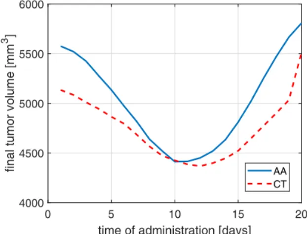
inputs, assuming aone-shotmonotherapy, namely we assume a protocol in which only one injection is administered from any of the drugs. We assume that the dose injected is 5 units ([mg/kg]). Figure 1 depicts the final volume (volume on final day 21) of the tumor as the function of one-shot administration time of the drug. For sake of comparison, the reference final tumor size (if no drug is administered) is 5848 mm3. Fig. 1 demonstrates that assuming one-shot monother- apy, both of the drugs (AA-antiangiogenic, CT-cytotoxic) affect the growth of the tumor on a similar magnitude, and both of them have an optimal administration time instance.
Furthermore, the model predicts that the angiogenic inhibitor is more sensitive to the exact time of administration, and that the optimal administration time of the cytotoxic drug can be found slightly later compared to the antiangiogenic drug (in accordance with medical knowledge).
0 5 10 15 20
time of administration [days]
4000 4500 5000 5500 6000
final tumor volume [mm3 ]
AA CT
Fig. 1. The final tumor volume as a function of the administration time, assuming one-shot monotherapy with a dose of 5 units in the case of the antiangiogenic (AA) and cytotoxic (CT) drug.
On the other hand, we may compare how the final tumor volume depends on the administered dose. Figure 2 depicts these results assuming that the corresponding dose is admin- istered on day 11 in order to achieve maximal effect. As we can see in these figures, the effect of the antiangiogenic drug is more saturating, while the effect of the cytotoxic drug depends more in a linear fashion on the administered quantity (again, in accordance with medical knowledge).
B. Interaction of drugs
If we apply both antiangiogenic and cytotoxic drug shots of 5 units at day 11, the simulation results in a final volume of 2924mm3, which clearly shows that the combination of the two drugs – according to model prediction – is more effective compared to the monotherapies. In fact, in Fig. 2, we can see that applying 10 units of the cytotoxic drug - which is the more effective at this dose -, compared to the 5-5 units of AA and CT, results in a final volume about 3600 mm3.
This can be explained by the saturation phenomena. If we individually increase the dose of either drug without applying the other, the increase of effect above a certain dose will not
0 5 10 15 20
applied dose [mg/kg]
2500 3000 3500 4000 4500 5000 5500
final tumor volume [mm3 ]
AA CT
Fig. 2. The final tumor volume as a function of the administered dose, assuming one-shot 21-day long monotherapy, where the administration time is day 11. The monotherapy was investigated for antiangiogenic (AA) and cytotoxic (CT) drug.
follow the increase of dose anymore, as it can be seen in Fig. 2. Furthermore, antiangiogenic drug has the potential to normalize the pathological tumor vasculature (vascular remodeling) and hence the cytotoxic drug can exerts its effect more efficiently [18], [19].
C. Open-loop protocols
In the following, we investigate discrete treatment proto- cols where a combination of antiangiogenic and cytotoxic drugs is administered for the patient in given days.
As both the cytotoxic and antiangiogenic drugs are typi- cally available as injections, and we assume outpatients, the number of days on which the patient must visit the hospital to get these injections can be considered as a critical parameter of the therapy, also significantly reflecting the load on the healthcare system.
In the following, considering fixed numbers of treatment days, we analyze how the treatment schedule and the distri- bution of the drug dosage among treatment days affects the efficiency of the therapy.
Table I summarizes the notations for the analyzed treat- ment schedules which were determined based on the follow- ing practical considerations:
• We assume 2-6 treatment days
• The interval between any two treatment days should be at least 2 days.
• We assume that in the initial period of tumor growth the tumor is unnoticed, thus the treatment may begin at earliest on day 6.
• Based on the results depicted in Fig. 1, we may con- clude that injections in the final phase of the tumor growth are not efficient, thus we assume that the last possible day for any schedule is day 16.
• We assume that the total injection quantity for the therapy is 5 units for both drugs.
• The minimal dose of injection is 0.1.
schedule days schedule days
S1 [6, 8] S30 [8, 12, 16]
S2 [6, 10] S31 [8, 14, 16]
S3 [6, 12] S32 [10, 12, 14]
S4 [6, 14] S33 [10, 12, 16]
S5 [6, 16] S34 [10, 14, 16]
S6 [8, 10] S35 [12, 14, 16]
S7 [8, 12] S36 [6, 8, 10, 12]
S8 [8, 14] S37 [6, 8, 10, 14]
S9 [8, 16] S38 [6, 8, 10, 16]
S10 [10, 12] S39 [6, 8, 12, 14]
S11 [10, 14] S40 [6, 8, 12, 16]
S12 [10, 16] S41 [6, 8, 14, 16]
S13 [12, 14] S42 [6, 10, 12, 14]
S14 [12, 16] S43 [6, 10, 12, 16]
S15 [14, 16] S44 [6, 10, 14, 16]
S16 [6, 8, 10] S45 [6, 12, 14, 16]
S17 [6, 8, 12] S46 [8, 10, 12, 14]
S18 [6, 8, 14] S47 [8, 10, 12, 16]
S19 [6, 8, 16] S48 [8, 10, 14, 16]
S20 [6, 10, 12] S49 [8, 12, 14, 16]
S21 [6, 10, 14] S50 [10, 12, 14, 16]
S22 [6, 10, 16] S51 [6, 8, 10, 12, 14]
S23 [6, 12, 14] S52 [6, 8, 10, 12, 16]
S24 [6, 12, 16] S53 [6, 8, 10, 14, 16]
S25 [6, 14, 16] S54 [6, 8, 12, 14, 16]
S26 [8, 10, 12] S55 [6, 10, 12, 14, 16]
S27 [8, 10, 14] S56 [8, 10, 12 ,14, 16]
S28 [8, 10, 16] S57 [6, 8, 10, 12, 14, 16]
S29 [8, 12, 14]
TABLE I
VARIOUS TREATMENT SCHEDULES TESTED FOR OPEN-LOOP THERAPY OPTIMIZATION
We compared two cases for each treatment schedule. In the first case we assumed that the drugs are evenly distributed among the days of the therapy; while in the second case, we assumed an optimal drug dosage. The optimal dosage problem was formulated as follows.
Let us denote the set of injections by I. Ikj ∈ I, stands for a single injection of one drug, where the upper indexj refers to the index of the injection day, and the lower index krefers to the type of the drug. The injection day has to be a treatment day:j∈D. If we denote the final volume of the tumor with VF, we can formulate an optimization problem:
minVF subject to X
j
Ikj ≤5 ∀ k (10) Ikj≥0.1 ∀ (j, k) , (11) where the last constraint corresponds to a minimal dose. We used particle swarm optimization algorithm [20] to minimize the the final volume of the tumor.
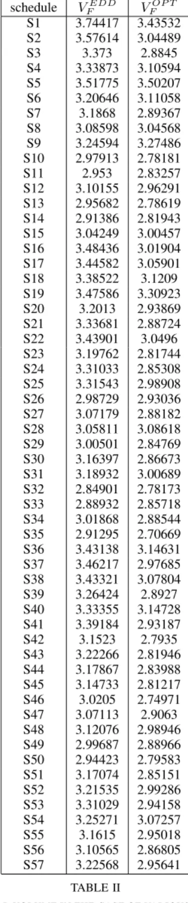
Table II summarizes the results corresponding to the various treatment schedules. We can see in this table that dosage optimization, compared to evenly distributed drug dosage, brings a significant benefit. The final volume of the tumor is 2.42 mm3 less in average assuming dosage optimization.
schedule VFEDD VFOP T
S1 3.74417 3.43532 S2 3.57614 3.04489
S3 3.373 2.8845
S4 3.33873 3.10594 S5 3.51775 3.50207 S6 3.20646 3.11058 S7 3.1868 2.89367 S8 3.08598 3.04568 S9 3.24594 3.27486 S10 2.97913 2.78181 S11 2.953 2.83257 S12 3.10155 2.96291 S13 2.95682 2.78619 S14 2.91386 2.81943 S15 3.04249 3.00457 S16 3.48436 3.01904 S17 3.44582 3.05901 S18 3.38522 3.1209 S19 3.47586 3.30923 S20 3.2013 2.93869 S21 3.33681 2.88724 S22 3.43901 3.0496 S23 3.19762 2.81744 S24 3.31033 2.85308 S25 3.31543 2.98908 S26 2.98729 2.93036 S27 3.07179 2.88182 S28 3.05811 3.08618 S29 3.00501 2.84769 S30 3.16397 2.86673 S31 3.18932 3.00689 S32 2.84901 2.78173 S33 2.88932 2.85718 S34 3.01868 2.88544 S35 2.91295 2.70669 S36 3.43138 3.14631 S37 3.46217 2.97685 S38 3.43321 3.07804 S39 3.26424 2.8927 S40 3.33355 3.14728 S41 3.39184 2.93187 S42 3.1523 2.7935 S43 3.22266 2.81946 S44 3.17867 2.83988 S45 3.14733 2.81217 S46 3.0205 2.74971 S47 3.07113 2.9063 S48 3.12076 2.98946 S49 2.99687 2.88966 S50 2.94423 2.79583 S51 3.17074 2.85151 S52 3.21535 2.99286 S53 3.31029 2.94158 S54 3.25271 3.07257 S55 3.1615 2.95018 S56 3.10565 2.86805 S57 3.22568 2.95641
TABLE II
FINAL TUMOR VOLUME IN THE CASE OF VARIOUS TREATMENT SCHEDULES,ASSUMING EVENLY DISTRIBUTED(VEDD
F )VS.OPTIMIZED (VOP T
F )DRUG DOSAGE
As one may see in Table II, the most efficient open-loop
therapy may be achieved with protocolS35. In this case the patient receives injections on days 12, 14 and 16 and the dosage is described in equation (12).
IAA12 = 2.36 IAA14 = 2.06 IAA16 = 0.58
ICT12 = 1.13 ICT14 = 0.33 ICT16 = 3.54 (12)
The final tumor volume is 2.707 mm3, while the drug concentrations resulting from the optimized injections are depicted in Fig. 3.
0 5 10 15 20
time [days]
0 1 2 3 4 5
drug concentrations [mg/kg]
AA CT
Fig. 3. Plasma drug concentrations in the case of the optimized dosage open-loop protocol.
D. Closed-loop therapy
The main motivation of the original bi-compartmental model [17] was the assumption that in the near future, biological markers which allow the estimation of the created state variables will be available for on-line measurements.
Assuming valid estimations for the state variables, different feedback laws can be designed for therapeutic purposes; fur- thermore, these closed-loop therapies will have the potential to be implemented when carry-on devices will be available for continuous administration of the drugs, as in the case of the artificial pancreas [13].
We introduce two heuristic proportional static feedback laws corresponding to the two drugs, based on biological considerations.
• The feedback of the antiangiogenic drug: As the process of angiogenesis is dependent on tumor angiogenesis factor (TAF) – the target of the antiangiogenic drug–, it is straightforward to assume that its inhibition makes sense only if TAF is present. As the function fT AF
describes the secretion rate of TAF by living tumor cells, it seems plausible to implement a feedback which is proportional to this normalized function as follows:
IAA(t) =KAAfT AF([NC(t)]) , (13) whereKAAis the corresponding feedback gain.
• The feedback of the cytotoxic drug: As the normalized actual growth rate function g([TP]), depending on the
tumor cell concentration in the periphery is a key element of tumor growth, and reflects the actual growth rate, it seems plausible to ’punish’ the tumor growth with the administration of cytotoxic drugs and formulate the corresponding feedback law as follows:
ICT(t) =KCTg([TP]) (14) whereKCT is the corresponding feedback gain.
Consequently, we consider two scenarios in the closed- loop case.
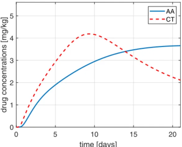
1) Limitation of the total injected drug amount: We investigate the case when the total injected amount of drugs in the closed-loop therapy is equal to the injection amount of the open-loop protocol (thus the total injection amount of both drugs is 5 units). As the simulations show that the total injected amount is a monotone increasing function of the feedback gain in the case of both drugs, we may easily determine feedback gains which result in this quantity, namely,KAA= 0.556andKCT = 0.633. Considering these feedback gains, the plasma drug concentrations will evolve as depicted in Fig. 4. This protocol results in the final tumor size of 3721mm3.
0 5 10 15 20
time [days]
0 0.5 1 1.5 2 2.5
drug concentrations [mg/kg]
AA CT
Fig. 4. The resulting plasma drug concentrations in the case of closed-loop administration, if the total injected quantity is equal to the open-loop case.
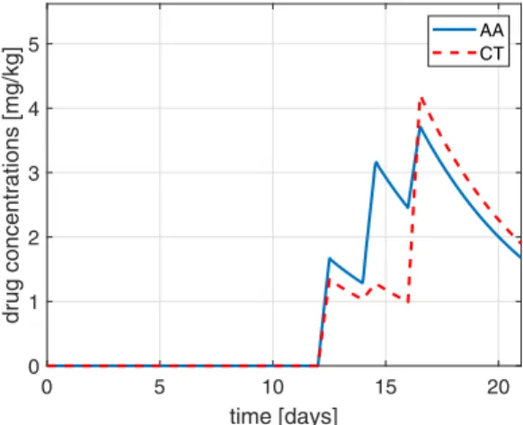
2) Limitation of the maximal plasma drug concentra- tion: From a pharmacotherapeutical point of view, maximal plasma concentration during the therapy can be used as quantification of drug load. In the optimal S35 open-loop therapy, maximal plasma concentration of the antiangiogenic drug is 3.7 mg/kg, and maximal plasma concentration of the cytotoxic drug is 4.2 mg/kg. Considering this therapy as basis to determine the feedback gains, we get the values KAA= 0.98 andKCT = 2.05. The dynamics of the drugs are depicted in Fig. 5 in this case.
As we can see in Fig. 5, neither of the drugs exceed the reference plasma concentrations. However, as the constant injection has to balance out clearance in this case, the total injected amounts are 13.39 units and 12.85 units for the antiangiogenic and for the cytotoxic drug respectively, which are significantly more compared to the original value of 5
0 5 10 15 20 time [days]
0 1 2 3 4 5
drug concentrations [mg/kg]
AA CT
Fig. 5. The resulting plasma drug concentrations in the case of closed-loop administration, if maximal plasma concentrations are equal to the open-loop case.
units. The final volume of the tumor however is only1879 mm3, which is only about 69% of the value obtained by optimal open-loop therapy.
IV. CONCLUSIONS AND FUTURE WORK In this paper, we extended the original model described in [17] with an additional input to make it able to account for cytotoxic drug application as well (in addition to the administration of angiogenic inhibitor). We have compared the effect of the two inputs to the dynamics of the model, and derived the optimal instance of one-shot therapy protocols for a reference drug injection value (5 units).
Regarding the open-loop protocol, we have formulated a simple drug-dosage optimization problem with a fixed number of injection days, and solved it with the help of numerical optimization. In addition, we analyzed a heuris- tic proportional static feedback law. If we constrained the total injected drug quantity, the proposed feedback control resulted in the final tumor size of 3721 mm3, which is equal to approximately 134% of the value obtained by the optimization of the open-loop protocol. On the other hand, if we constrained the maximal plasma concentration of the injected drugs according to the optimal scenario in the open- loop approach, the final volume of the tumor reduced to1879 mm3, which is only about 69% of the optimal open-loop reference value. This result clearly shows the potential of closed-loop approaches according to model predictions.
We have to note that the model [17] has been validated only with tumor volume measurements, and not yet with dynamical vasculature data, so its predictions must be con- sidered in the light of this. However, on the other hand we, are not aware of any dynamical model in the literature which would have been validated against such explicit data.
In the future, we will focus on robustness analysis as a straightforward continuation of the work performed in this article. As the main expectation of closed-loop control is to cancel out model uncertainties at considerable level, it
would be desirable to study how parametric changes affect the optimality of open- and closed-loop approaches.
REFERENCES
[1] J. Folkman, “Tumor angiogenesis: therapeutic implications,” New england journal of medicine, vol. 285, no. 21, pp. 1182–1186, 1971.
[2] A. Abdollahi and J. Folkman, “Evading tumor evasion: current concepts and perspectives of anti-angiogenic cancer therapy,” Drug Resistance Updates, vol. 13, no. 1, pp. 16–28, 2010.
[3] J. S´api, L. Kov´acs, D. A. Drexler, P. Kocsis, D. Gaj´ari, and Z. S´api,
“Tumor volume estimation and quasi-continuous administration for most effective bevacizumab therapy,”PloS ONE, vol. 10, no. 11, p.
e0142190, 2015.
[4] D. Hanahan and J. Folkman, “Patterns and emerging mechanisms of the angiogenic switch during tumorigenesis,”Cell, vol. 86, no. 3, pp.
353–364, 1996.
[5] S. R. McDougall, A. R. Anderson, and M. A. Chaplain, “Mathematical modelling of dynamic adaptive tumour-induced angiogenesis: clinical implications and therapeutic targeting strategies,”Journal of theoreti- cal biology, vol. 241, no. 3, pp. 564–589, 2006.
[6] H. Rieger and M. Welter, “Integrative models of vascular remodel- ing during tumor growth,”Wiley Interdisciplinary Reviews: Systems Biology and Medicine, vol. 7, no. 3, pp. 113–129, 2015.
[7] R. K. Jain, “A single-cell-based model of tumor growth in vitro:
monolayers and spheroids,” Nature Medicine, vol. 7, pp. 987–989, 2001.
[8] EU, “Directive 2010/63/EU of the European Parliament and of the Council of 22 September 2010 on the protection of animals used for scientific purposes ,”Official Journal of the European Communities, vol. L276, no. 63, pp. 33–80, 2010.
[9] H. F. Zhang, K. Maslov, G. Stoica, and L. V. Wang, “Functional photoacoustic microscopy for high-resolution and noninvasive in vivo imaging,”Nature Biotechnology, vol. 24, no. 7, pp. 848–851, 2006.
[10] B. J. Vakoc, R. M. Lanning, J. A. Tyrrell, T. P. Padera, L. A. Bartlett, T. Stylianopoulos, L. L. Munn, G. J. Tearney, D. Fukumura, R. K. Jain et al., “Three-dimensional microscopy of the tumor microenvironment in vivo using optical frequency domain imaging,” Nature Medicine, vol. 15, no. 10, pp. 1219–1223, 2009.
[11] P. M. Gignac, N. J. Kley, J. A. Clarke, M. W. Colbert, A. C. Morhardt, D. Cerio, I. N. Cost, P. G. Cox, J. D. Daza, C. M. Earlyet al., “Dif- fusible iodine-based contrast-enhanced computed tomography (dicect):
an emerging tool for rapid, high-resolution, 3-d imaging of metazoan soft tissues,”Journal of Anatomy, vol. 228, no. 6, pp. 889–909, 2016.
[12] J. S´api, D. A. Drexler, and L. Kov´acs, “Potential benefits of discrete- time controllerbased treatments over protocol-based cancer therapies,”
Acta Polytechnica Hungarica, vol. 14, no. 1, pp. 11–23, 2017.
[13] F. J. Doyle, L. M. Huyett, J. B. Lee, H. C. Zisser, and E. Dassau,
“Closed-loop artificial pancreas systems: engineering the algorithms,”
Diabetes Care, vol. 37, pp. 1191–1197, 2014.
[14] H. Blauw, P. Keith-Hynes, R. Koops, and J. H. DeVries, “A review of safety and design requirements of the artificial pancreas,” Annals of Biomedical Engineering, vol. 44, no. 11, pp. 3158–3172, 2016.
[15] L. Kov´acs, “Linear parameter varying (LPV) based robust control of type-I diabetes driven for real patient data,”Knowledge-based Systems, vol. 122, pp. 199–213, 2017.
[16] A. Borri, P. Palumbo, C. Manes, S. Panunzi, and A. De Gaetano,
“Sampled-data observer-based glucose control for the artificial pan- creas,”Acta Polytech. Hungarica, vol. 14, no. 1, pp. 79–94, 2017.
[17] D. Csercsik, J. S´api, T. G ¨onczy, and L. Kov´acs, “Bi-compartmental modelling of tumor and supporting vasculature growth dynamics for cancer treatment optimization purpose,” in 56th IEEE Annual Conference on Decision and Control (CDC), Melbourne, Australia, 2017, pp. 4698–4702.
[18] J. Ma and D. J. Waxman, “Combination of antiangiogenesis with chemotherapy for more effective cancer treatment,”Molecular cancer therapeutics, vol. 7, no. 12, pp. 3670–3684, 2008.
[19] I. F. Nerini, M. Cesca, F. Bizzaro, and R. Giavazzi, “Combination therapy in cancer: effects of angiogenesis inhibitors on drug pharma- cokinetics and pharmacodynamics,”Chinese journal of cancer, vol. 35, no. 1, p. 61, 2016.
[20] A. I. F. Vaz and L. N. Vicente, “A particle swarm pattern search method for bound constrained global optimization,”Journal of Global Optimization, vol. 39, no. 2, pp. 197–219, 2007.