How to design a transdisciplinary regional ecosystem service assessment: a case study from Romania, Eastern Europe

(1)

Ecosystem Service Mapping

How to design a transdisciplinary regional

ecosystem service assessment: a case study from Romania, Eastern Europe

Bálint Czúcz , Ágnes Kalóczkai, Ildikó Arany, Katalin Kelemen, Judith Papp, Krisztina Havadtői, Krisztina Campbell, Márton A. Kelemen, Ágnes Vári

‡ MTA Centre for Ecological Research, Klebelsberg K. u. 3, H-8237 Tihany, Hungary

§ European Topic Centre on Biological Diversity, Muséum national d’Histoire naturelle, 57 rue Cuvier, FR-75231 Paris, Paris Cedex 05, France

| Milvus Group Association, Crinului Str. 22, 540343 Targu Mures, Romania

¶ Executive Agency for Small and Medium-sized Enterprises, European Commission, Place Charles Rogier 16, 1210 Saint- Josse-ten-Noode Brussels, Belgium

Corresponding author: Bálint Czúcz (czucz.balint@okologia.mta.hu) Academic editor: Davide Geneletti

Received: 02 May 2018 | Accepted: 28 Aug 2018 | Published: 31 Aug 2018

Citation: Czúcz B, Kalóczkai Á, Arany I, Kelemen K, Papp J, Havadtői K, Campbell K, Kelemen M, Vári Á (2018) How to design a transdisciplinary regional ecosystem service assessment: a case study from Romania, Eastern Europe. One Ecosystem 3: e26363. https://doi.org/10.3897/oneeco.3.e26363

Abstract

There is a broad diversity of concepts and methods used in ecosystem service (ES) mapping and assessment projects with many open questions related to the implementation of the concepts and the use of the methods at various scales. In this paper, we present a regional ES mapping and assessment (MAES) study performed between 2015 and 2017 over an area of ~900 km in Central Romania. The Niraj-MAES project supported by EEA funds and the Romanian government aimed at identifying, assessing and mapping all major ES supplied by the Natura 2000 sites nested in the valleys of the Niraj and Târnava Mică rivers amongst the foothills of the Eastern Carpathians. Major ES in this culturally and ecologically rich semi-natural landscape were determined and prioritised in cooperation with local stakeholders. Indicators for the capacities of individual services were modelled with a multi-tiered methodology, relying on the involvement of regional thematic experts. ES with appropriate socio-economic data were also evaluated economically. The whole

‡,§ ‡ ‡ | | |

¶ | ‡

2

© Czúcz B et al. This is an open access article distributed under the terms of the Creative Commons Attribution License (CC BY 4.0), which permits unrestricted use, distribution, and reproduction in any medium, provided the original author and source are credited.

(2)

process was supervised by a stakeholder advisory board endowed with a remarkable decision-making position, giving feedback and recommendations to the scientists at the critical nodes of the process, thus ensuring salience and legitimacy. In addition to simply presenting the dry facts about the approaches (assessment targets, methods) and outcomes, we also identify several key decisions on the design of the whole assessment process related to (1) the role of conceptual frameworks, (2) stakeholder involvement, (3) the selection of ES to assess (priority setting), (4) the development of models and indicators and (5) the interpretation of outcomes, for which we give a detailed description of the decision process. We found that conceptual frameworks can have a pivotal role in structuring and facilitating communication amongst the participants of a MAES project and that a broad and structured involvement of stakeholders and (local) experts creates a sense of ownership and thus can facilitate local policy uptake. We argue that priority setting and the development of indicators should be an iterative process and we also give an example how such a process can be designed, enabling an eﬃcient participation of a broad range of experts and the collaborative development of simple ES models and indicators. Finally, we discuss several general issues related to the interpretation of results of any kind of MAES and the follow-up of regional MAES projects.

Keywords

MAES, ecosystem assessment, conceptual framework, mapping, transdisciplinarity, ecosystem condition, participatory approach

Introduction

Ecosystem services (ES) improve people’s individual and social well-being in many ways (MA 2005) and are indispensable for the healthy functioning of society and economy and their building blocks: local communities. In spite of this, we are losing ES at an alarming rate (Cardinale et al. 2012). Short-sighted decisions damage ‘nature’s free goods’, as concluded by a Transylvanian decision-maker in as early as 1786 (Molnár et al. 2015) in Sfântu Gheorghe, Romania - very close to the region where the ecosystem assessment presented in this paper took place. Amid the enormous environmental challenges of the 21

century, this conclusion is more relevant today than it has ever been.

One of the reasons for society not being able to solve today’s environmental crisis is the

‘traditional’ way how society handles natural resources and environmental issues (Loorbach 2007). Each ‘sector’ is managed separately, by dedicated governance institutions, none of which has either the capacities or the mandates to handle overarching effects (Lyall and Tait 2005). A potential solution to this problem builds on the concept of ES that can serve as a boundary object (Star and Griesemer 1989) connecting the different sectors. Ecosystem service assessments offer a common platform to break down the silos and harmonise the otherwise isolated sectoral policies (Díaz et al. 2015). It is no surprise that the ES concept has been integrated into the most recent environmental / natural

st

(3)

resource policies worldwide and there are several key policies addressing ES assessments speciﬁcally at an international and EU level (e.g. CBD’s Aichi Targets and the EU Biodiversity Strategy). A quantitative integration of ES into economic accounts (like GDP) is a major policy goal (Guerry et al. 2015), which could greatly inﬂuence all aspects of political and economic decision-making. Furthermore, mainstreaming the ES concept into general public communication (and enabling people to ‘think in ES’) can increase coping and problem-solving capacities (resilience) at a societal level (Díaz et al. 2015).

In this paper, we present and discuss several key ‘design questions’ of regional ecosystem assessment studies using a complex regional ES assessment as a case study. We present the Niraj-MAES assessment performed between 2015 and 2017 over an area of ~900 km in Central Romania focussing primarily on the design decisions determining the assessment structure and the methods used. We lay particular emphasis on a few selected key aspects (“topics”) of the assessment process:

• (Topic 1): the various roles of the conceptual framework (ranging from structuring the process to facilitating the communication, as discussed by, for example, Potschin-Young et al. 2018);

• (Topic 2): the involvement of stakeholders and the integration of diﬀerent knowledge forms (including stakeholder perceptions, unformalised expert knowledge, scientiﬁc literature and conceptual frameworks, e.g. Díaz et al. 2018, Dick et al. 2018);

• (Topic 3): the selection of assessment priorities (including the decision on ES to be assessed) and the underlying process criteria (e.g. Ramirez-Gomez et al. 2015, Oudenhoven et al. 2018);

• (Topic 4): the methods (models and indicators) available for quantifying ES and the criteria for choosing amongst them (selection criteria, as well as process criteria, e.g. Harrison et al. 2018, Wainger and Mazzotta 2011); and

• (Topic 5): the integration of the diverse outcomes (ES models, maps, monetary values) into a common framework and the potential issues related to the interpretation of the outcomes (e.g. Dick et al. 2018, Olander et al. 2017).

In all of these key topics, we had to make serious design decisions during our assessment process, for which we could not ﬁnd any easily accessible guidance in literature. Thus we made our own research, evaluated the options and brought our own decisions, and we learned a lot during this process. We think that our lessons can help others in similar situations and thus are interesting for the broad MAES community. Accordingly, in the following chapters we will

• present the workﬂow of the Niraj-MAES assessment step-by-step, from the description of the assessment site and targets to the methods and indicators used for mapping to the ﬁnal results of the assessment; and

2

(4)

• integrate considerations (descriptions of the decision context, approaches considered and our final decision with justification) related to the five key topics highlighted above into the presentation of this workflow.

We do not intend to go into methodological details in any of the assessment steps with complex theoretical backgrounds (e.g. economic valuation), but we intend keeping the focus of the presentation on the structural design of the assessment process. Similarly, the primary outputs of the assessment process (indicators maps, monetary results) are also presented very brieﬂy, only to the degree that is necessary to illustrate the methodological choices. The paper is concluded by ample discussion on the ﬁve key topics highlighted above.

Materials and Methods

Study area

The study area consists of four partly overlapping Natura 2000 areas (ROSCI0384, ROSCI0297, ROSCI0186 and ROSPA0028) comprising ~91,000 ha at the foot of the Eastern Carpathians between 301 m and 1080 m a.s.l. in South-East Transylvania, Romania. There are altogether ~203,000 inhabitants (average population density 68/km ) with 13% of the population concentrated in the six cities of the region. Settlements are mostly located along the two main rivers, the Niraj and the Târnava Mică. While agriculture is still a dominant source of income, oﬃcial data show that few people earn their living from this economic sector. The relatively high share of natural and semi-natural habitats gives the landscape a ‘wild’ character, a consequence of the traditional land management practices that have been in use until very recently and can still be found in some parts of the study area. However, despite the deep aﬀection the locals might have for the landscape, migration to urban areas is increasing, as better job and education opportunities are available there.

The vegetation has a transitional character between the lowland and the mountain regions of the Eastern Carpathians. The area is dominated by forests and pastures that were grazed traditionally by cattle, but nowadays rather by sheep. There has been an increasing tendency for land abandonment resulting in transient shrublands (encroached grasslands) in the place of former pastures, hay meadows or arable fields. Some of the hay meadows are still used for winter fodder production in cattle and sheep husbandry. Agricultural fields typically consist of a high number of small parcels reflecting historical land use and property systems, but larger plots cultivated by intensive modern agricultural techniques can also be found in the broad river valleys. Of the two main rivers, Târnava Mică is more natural, with broad meanders and gallery forests. The natural bed of the Niraj has mostly been destroyed in a series of recent riverbed corrections. Due to the lost meanders, the slope of the Niraj river has increased significantly, leading to strong erosion of the banks and a series of follow-up correction works.

2

(5)

Assessment principles

Conceptual framework (Topic 1)

Throughout the assessment, we adhered to a conceptual framework (CF, Fig. 1) that can be seen as a customised and further operationalised version of the CF underlying the recommendations of the EU MAES working group (Maes et al. 2013, Maes et al. 2014) and the integrated ecosystem assessment (IEA) framework (Burkhard et al. 2018, Brown et al.

2018, Fig. 2) developed in the framework of the ESMERALDA project (Burkhard 2018). We considered the most important roles of our CF that

• it creates a clear structure for the process of our work and the communication of our results,

• it ensures compatibility with other similar assessments performed elsewhere and

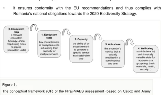
• it ensures conformity with the EU recommendations and thus complies with Romania’s national obligations towards the 2020 Biodiversity Strategy.

Following the ES cascade model (Potschin and Haines-Young 2011; La Notte et al. 2015;

Czúcz and Arany 2016) underlying the MAES and ESMERALDA recommendations, our CF (Maes et al. 2014; Burkhard et al. 2018; Fig. 1) represents the various stages of the ﬂow of the services from nature towards society. The starting point is rather technical: we need to have a spatially explicit account of what kind of ecosystems there are in the study area, which is represented by an ecosystem type map (level 0), classifying each land unit into the categories of an ecosystem typology perceived as meaningful by the locals. These ecosystems can be characterised with respect to a number of ecosystem condition aspects (level 1) that fundamentally determine their internal processes and operation. Appropriate condition enables ecosystems to provide services (capacity, level 2). However, the capacity of ecosystems to provide certain services is not the same as the services actually used (

Figure 1.

The conceptual framework (CF) of the Niraj-MAES assessment (based on Czúcz and Arany 2016), indicating consecutive steps of the assessment process.

(6)

actual use, level 3) as the latter can be influenced by societal needs, ‘demand’ at a given place and time, as well as the human inputs expended to obtain services. The benefits of the services used then appear in the form of maintained or increased well-being in society (level 4, see all definitions in Suppl. material 1).

Figure 2.

Matching the MAES assessment framework (a; Maes et al. 2014) and the ESMERALDA integrated ecosystem assessment framework (b; Burkhard et al. 2018) to our cascade-based conceptual framework (c; Fig. 1) and to our workﬂow (d; Fig. 3).

(7)

The key steps of this pathway define ‘entry points’ for interpreting and ‘measuring’ the flow of services from nature towards society. To implement this framework, we substantiated what kind of information we intended to assess at each level of this modified cascade framework (Table 1).

Cascade level Thematic dimension Desired number of indicators Spatial resolution

0. ecosystem map ecosystem types 1 (a single map) full (100 x 100 m)

1. ecosystem condition

condition aspects 1(-2) per condition aspect full (100 x 100 m)

2. capacity ecosystem services 1(-2) per ES full (or

aggregated) 3. actual use ecosystem services (1-)2 per ES (1 monetary and 1(-2)

biophysical)

aggregated (or full)

4. beneﬁts ES, well-being dimensions

few (1 per ES and well-being dimension) aggregated

To further implement the CF, we also created working definitions for several key concepts based on literature definitions and conscious harmonisation (Suppl. material 1). In line with these definitions, we also set down our attitude towards several 'hot questions' of ecosystem assessment practice discussed in the CICES manual (Haines-Young and Potschin 2018). For example, abiotic services (i.e. goods and services provided directly by the non-living physical environment without the assistance of biota, like mineral salts or extracted drinking water) were not considered as ecosystem services. We also excluded products derived from strongly transformed and principally human-controlled ‘industrial ecosystems’ (e.g. crops from intensive agriculture) which we considered to be on the

‘human side’ of the production boundary (Haines-Young and Potschin 2018), for several reasons:

• as the process generating such goods is fundamentally governed by human management (through the above-mentioned inputs), the conceptual framework applied in this study (Fig. 1) would be very poorly applicable for the description and analysis of such services;

• such goods require vast amounts of material and energy inputs from man (e.g.

fertilisers, pesticides, agricultural machinery, fuel) which might easily exceed the contributions of natural systems to the production process (see, for example, the calculations in Bengtsson 2015);

Table 1.

Assessment goals as deﬁned by the conceptual framework (CF): the type of information (number and type of indicators and the underlying typologies) sought by Niraj-MAES for each element of the CF.

(8)

• contributions from natural ecosystems to agricultural production (e.g. pollination, pest control, soil fertility) are often considered to be (regulating) ES in their own right and taking into account both the regulating ES and the ﬁnal crops as ES would qualify as double-counting (Boyd and Banzhaf 2007); and

• agricultural goods constitute economic products that are already well represented in the currently existing economic accounts, so there is relatively little added value in (re)calculating / relabelling these already known values.

Accordingly, we considered such agricultural goods as internal products of the economy to which natural ecosystems contribute only indirectly, through other services (e.g. ensuring pollination, natural plant protection, maintaining soil fertility). Being potentially the most relevant, ‘soil fertility’ was chosen to be included in our assessment (compare also Albert et al. 2016; Rabe et al. 2016).

Participatory approach (Topic 2)

The use of scientiﬁc information for policy and resource management purposes should not be considered as a one-way knowledge transfer. A better model for the relationship of science and society in this process is that of a ‘joint knowledge production’ (Turnhout et al.

2007). From a policy perspective, the success of a research project resides in the use of its results by policy actors, influence on policy processes and impact on policy outcomes (Bauler 2012). It is actually the perception by key local, regional and national stakeholders (or policy actors) that determines the uptake of research results. There are three key components determining success in this respect: credibility (=scientific and technical suitability), salience (=ability to address user concerns) and legitimacy (=the political acceptability or perceived fairness of the process; Cash et al. 2003). In order to become influential, the research process needs to be perceived simultaneously and consensually as being legitimate, credible and salient by major groups of stakeholders (Bauler 2012).

These criteria depend not only on the objective characteristics of the methods applied, but also on the perceptions of the relevant stakeholders. Accordingly, the research process should be considered as important as the results themselves, which is a common characteristic of post-normal science (Funtowicz and Ravetz 1993). Perceptions of credibility, salience and, particularly, legitimacy can be ensured by thorough stakeholder involvement throughout the research process. Intensive stakeholder involvement can also be considered as an example of extended peer review as proposed by Funtowicz and Ravetz (1997).

In this project, we aimed at involving a broad variety of stakeholders throughout the entire research process. The two main roles of the stakeholders (sensu lato) were:

• to help to deﬁne priorities (what is perceived as relevant and what is negligible from the perspective of the local population) and thus ensure politically and socially relevant results; and

(9)

• to assist in gaining a good system understanding (knowledge elicitation, how the diﬀerent components of local society are interlinked with nature and economy).

In the second case (knowledge elicitation), the participating stakeholders were mostly selected according to their knowledge and expertise (local experts), while for the ﬁrst case (prioritisation) opinions of the whole local population were regarded as relevant. We thus distinguished two ‘target groups’ for involvement: local experts with a thematic mandate related to their ‘expertise’ (that does not need to be based on formal training, in this context even an illiterate shepherd with a lot of traditional ecological knowledge can be considered as a local expert in grazing) and stakeholders (sensu stricto) that involves all locals, visitors and everyone else who has a stake in the well-functioning of the regional socio-ecological system. The involvement of local experts enabled us to capture complex nature-society relationships in the form of simple, but (locally) relevant models.

As a key element of making the Niraj-MAES research approach participatory, we relied on the help of an 'Advisory Board', comprising locals representing the most important economic and social sectors of the area (Box 1 in Suppl. material 2). The Advisory Board

‘supervised’ the entire assessment process, thus ensuring salience and legitimacy: every important step and result of the study was discussed with them and their suggestions were incorporated into the analyses, models and evaluations. The mapping and assessment process included, however, several further ‘participatory steps’ which had a vital inﬂuence on the outcome and success of the Niraj-MAES project, including an initial stakeholder analysis (Box 2 in Suppl. material 2), two ES prioritisation campaigns (Box 3 in Suppl.

material 2) and a scenario planning exercise (Box 4 in Suppl. material 2).

To make the stakeholder involvement process equally as important as the results, leaders of the research had to be open-minded and reﬂect the needs of the stakeholders. The cooperation with the stakeholders started at the beginning of the research and was implemented by a locally embedded non-governmental organisation.

Assessment workflow

The structure of the research project that we designed, based on the guiding principles discussed above, is presented in Fig. 3. The scenario planning exercise, mentioned above, is not directly related to the implementation of ecosystem service mapping and assessment (MAES assessment) as put forward in the EU MAES working group recommendations (Maes et al. 2013, Maes et al. 2014). This is reflected by the fact that this exercise constitutes a relatively independent secondary strand of the project workflow, parallel to the MAES assessment. This paper primarily focuses on the process and results of the first strand, the MAES assessment process, while the stakeholder planning strand is described in detail in Kalóczkai et al. 2017 and Arany et al. 2016.

The MAES assessment process predominantly follows the logic of the conceptual framework (Fig. 1) and the recommendations of the EU MAES working group, thus providing relevant results for high-level (regional, national and EU) policies. The complementary scenario planning process, on the other hand, primarily addresses the

(10)

local level, involving broad groups of the local community. Accordingly, we considered the scenario planning strand as an equally important key element of the Niraj-MAES process, which can create an interest in the ES concept and the assessment process (Palomo et al.

2011) and enhance the exploration of future options for decision-making (Albert et al.

2017). The two strands are, however, interlinked at a few key nodes to maximise synergies (Fig. 3).

Setting assessment focus (Topic 3)

The selection of ES and the methods and indicators to measure them was done in an iterative process, gradually reducing the thematic scope of the assessment to a feasible set of well-deﬁned ecosystem service indicators. This focus-setting process consisted of two main steps:

• I: selecting / specifying the main 'topics' for the ES assessment (=the ES to be assessed);

• II: implementing these topics by linking them to more speciﬁc indicators (=data and methods).

Selecting the services to be assessed

In order to make the ES assessment as locally relevant as possible, we started out with methods capturing the ES perception and priorities of a very broad range of local stakeholders (Kelemen et al. 2017), in an ES prioritisation process consisting of 3 main steps:

• from the initial interviews of the stakeholder analysis (Box 2 in Suppl. material 2), we extracted a list of 'ES-candidates' (topics mentioned that can potentially be considered as ES);

Figure 3.

The main workﬂow of the Niraj-MAES project, with major steps of the assessment process (Strand 1) linked to the boxes of the conceptual framework (numbers in parentheses, with bold numbers indicating primary focus (see Fig. 1).

(11)

• these ES-candidates were then discussed and scored by the Advisory Board (Box 1 in Suppl. material 2) and an 'ES-shortlist' was selected; and

• the shortlisted ES were ﬁnally ranked in a general preference assessment exercise (Box 3 in Suppl. material 2).

Based on individual rankings, we drew up an aggregated ranking of the services, describing the relative ‘value’ that the local population assigns to the diﬀerent ES. The ranked ES shortlist, established through this process, was then revised, based on conceptual and technical considerations and discussed with the Advisory Board.

Selecting methods and indicators

For each ES valued by the locals as important to be included in the assessment, a matching indicator is needed that actually represents the service as closely as possible.

For some services, this is a rather trivial choice, while, for others, some abstractions, combinations or speciﬁcations of certain aspects have to be made. To select indicators for ES mapping, we started out from both the results from the preference assessment process and the few ‘predeﬁned’ ES that were named in our grant proposal (agricultural crop production, hay production, provisioning services from semi-natural ecosystems, carbon sequestration, habitat for biodiversity, recreational potential). Based on a number of methodological and conceptual considerations, several shortlisted ES were merged and some were considered to be most feasibly represented with condition indicators (Suppl.

material 3). The indicators (as well as the underlying services / condition aspects) were then deﬁned more precisely and appropriate methods were also identiﬁed for modelling them (Table 2). The selection criteria underlying our two-step decision process are summarised in Table 3.

short name

long name deﬁnition of the ES indicator cascade level

modelling approaches CICES 5.1 classes

naturalness habitat naturalness

The "naturalness" (incl. biodiversity and resilience) of the habitat. This ecosystem state inﬂuences the provision of several ecosystem services within and beyond the ones studied in this project, e.g. pest control, disease control, pollination.

1 statistical model (a Tier 2 index based on the modelled occurrence probabilities of some taxonomical groups of conservational signiﬁcance)

-

Table 2.

The list of ES indicators and ecosystem condition indicators selected for mapping in the Niraj- MAES project. Modelling approaches show the directions planned for model development at the stage of the ES selection, final models & indicators are specified in Table 6. CICES classes notifications follow Haines-Young and Potschin (2018).

(12)

short name

landiv landscape diversity

The habitat diversity of the broader landscape, which contributes to the persistence of several plant and animal species, as well to an aesthetically appealing environment.

1 statistical model (a Tier 2 landscape index: the diversity of broad habitat types under a moving window)

-

fertility soil fertility Fertility of the soil is a semi-persistent ecosystem state aﬀecting the supply of several ES. In case of agro-ecosystems, it determines the ecosystem's potential contribution to the agricultural yield.

1 expert scores based on primary data (Soil Map of Romania (Harta Solurilor 1978))

-

hay natural forage and fodder

Potential forage supply provided by the ecosystems through mowing or grazing.

Cultivated or marketed roughage and grain feed are not included while grazing on fallow land and stubble as well as plants spontaneously occurring on waysides and banks are included in this service.

2 (1) matrix model (a Tier 1 statistical model based on expert scores and a habitat map)(2) enhanced matrix model (a Tier 2 statistical model with additional expert rules

1.1.3.1, 1.1.3.2

timber wood and timber

Long-term timber and ﬁrewood provisioning potential of the habitat, assessed as a yearly average considering the whole lifecycle of the habitat, not taking eﬀects of climate change into account.

2 (1) matrix model (a Tier 1 statistical model based on expert scores and a habitat map)

(2) enhanced matrix model (a Tier 2 statistical model based on forestry production tables (Tabele de producție (Giurgiu et al.

2004))

1.1.5.2, 1.1.5.3

berry medicinal and edible plants and mushrooms

Gathered mushrooms, fruits, berries and medicinal herbs provided spontaneously by the habitat. Cultivated plants and mushrooms are not included.

(2) enhanced matrix model (a Tier 2 statistical model based on structured exploration of plant habitat preferences)

1.1.5.1

honey honey provision and pollination

Potential of the habitat to supply nectar and pollen for honeybees and so contribute to honey production.

(2) enhanced model (a Tier 2 statistical model based on habitat types and slope categories)

1.1.3.1

(13)

short name

erosion water retention

& erosion control

Contribution of the land cover to slowing down the passage of surface water and thus to the recharge of regional groundwater resources and the mitigation of soil erosion.

(2) enhanced model (a Tier 2 statistical model based on habitat types and slope categories)

2.2.1.1

carbon carbon sequestration

Sequestration and storage of atmospheric carbon by the habitat, as contribution to global climate change mitigation.

2-3 IPCC model (adapting a Tier 1 IPCC national greenhouse gas inventory model to the Niraj-MAES area)

2.2.6.1

tourism tourism and local identity

Contribution of the habitat to the touristic attraction value of the area. Habitats allow recreation and create emotional bond in local people.

(2) enhanced model (an ESTIMAP-style Tier 2 statistical model based on the matrix model &

additional rules)

3.1.1.1, 3.1.1.2, 3.1.2.4, 6.1.1.1

criteria phase CSL

addressed

examples from Niraj-MAES

should meet stakeholder preferences / interests

I legitimacy, salience

stakeholder analysis, preference assessment, SAB supervision

should meet policy interests I salience, legitimacy

sponsor expectations from grant call and promises in our grant proposal; SAB expressing local sectoral

expectations/interests should match conceptual

considerations

I salience,

credibility

match to CF elements, exclusion of certain topics “based on MAES and CICES recommendations”

should measure what it states to measure

II credibility, salience

meticulous ES and indicator deﬁnitions with an eye to data and methods, emphasised throughout all consultative steps and reﬁned iteratively

Table 3.

Two sets of criteria for identifying indicators for the ES assessments. Phase I: criteria for selecting the 'topics' for which we need indicators; Phase II: criteria for selecting speciﬁc indicators (=data and methods) for each topic. CSL means credibility, salience and legitimacy; see Cash et al.

(2003).

(14)

criteria phase CSL addressed

examples from Niraj-MAES

should be supported by relevant expert opinion / knowledge

II credibilty, legitimacy

expert workshops / consultations, SAB meetings; the involvement of local experts also considered to “assist in gaining a system understanding”

understandability, ease of communication

II salience transparent modelling techniques were favoured wherever possible, structured and thorough communication of all elements (indicator deﬁnitions, map explanations etc.) data and methods

availability

I, II practical consideration

a very pragmatic criterion strictly applied throughout the ES identiﬁcation and methods selection process

time and resource constraints

II practical consideration

this made us exclude several options, e.g. Tier 3 models

Mapping and valuation

In the previous section, we have shown how we determined the questions and approaches in the focus of our assessment. In this section, we give a concise account of the speciﬁc data and methods we used, following the structure and logic set out in the Niraj-MAES conceptual framework (Fig. 1, Table 1).

Ecosystem map

The key input data layer consistent with the initial node of the Niraj-MAES conceptual framework is an ecosystem type map, classifying the study area into fundamental functional units (ecosystem / habitat types: level 0 in Fig. 1, see also Maes et al. 2014, and Suppl. material 1 for more precise deﬁnitions used). As there was no good quality ecosystem / habitat map readily available for our study area, we created our own map from scratch, based on the following data sources:

• Google Satellite and Google Streets and Terrain layers (from the ‘open layers’

plugin of QGIS);

• a land use map (own data from a previous project);

• forest maps and data (oﬃcial forestry administration data – but just for a few sites with Natura 2000 forest types).

To generate the ecosystem map, we first drafted an initial set of ecosystem types based on previous ES assessment experiences and our own understanding of the region’s landscape. This initial ecosystem typology was then gradually further specified and refined

(15)

based on input from our expert groups, as we progressed with the generation of the ecosystem map. The most important principles of this process were the following:

• the typology should be ﬁne enough to reﬂect local reality (all major functional units of the Niraj-Târnava Mică landscape should be distinguished); but

• the individual types should be clear and well-deﬁned, forming a coherent and easily understandable (logical) set together;

• the whole process should be feasible (given the available data and human resources); and

• the ﬁnal typology should be compatible with the MAES ecosystem typology (Maes et al. 2013).

The ﬁnal ecosystem map assigns the dominant ecosystem types to each basic spatial unit of the study area (‘pixels’ of 100 x 100 m). The map was generated with QGIS (Quantum Gis 2.10.1. Pisa; QGIS 2016) in the Dealul Piscului 1970/Stereo70 coordinate reference system (the national CRS for Romania) and further reﬁned in ArcGIS version 10.2 (ESRI 2011).

Spatial modelling (Topic 4)

In order to create maps of the ecosystem condition (level 1 in Fig. 1) or services (level 2), spatial data are needed. Such data can be either

• external data from public data sources (whenever spatial data with an appropriate thematic, spatial scope and resolution are available for the project); or

• modelled data (in all other cases – relying on loosely related external data and appropriate methodologies).

Models link biophysical data spatially represented by input maps with variables (indicators) describing the ecosystems with respect to a speciﬁc aspect of their condition or their capacity to provide a certain ES. In our work, we used models of three major model types:

matrix models (tier 1 models), rule-based models and statistical models (latter two: tier 2 models, Grêt-Regamey et al. 2015, Grêt-Regamey et al. 2018).

Due to their simplicity and flexibility, matrix models are a particularly popular ES assessment technique (Burkhard et al. 2010, Jacobs et al. 2015). The only spatial input to the model is an "ecosystem map" (which is a simple categorical map relying on a locally relevant ecological (habitat), land use (management) and/or land cover classification) of the study area. The model itself is no more than a simple look-up table (‘matrix’) which links the ecosystem types to indicator scores. Matrix models are ideal for participatory model building involving local experts, but there are also several other ways to populate the matrix with scores (e.g. Bagstad et al. 2013). While participation gives the benefit of involving

(16)

locals and enhancing uptake of results, this very simple approach might not reﬂect the complex processes underlying ES and the generation of ES precisely enough.

Rule-based models are an extension to matrix models. By identifying additional relevant spatial input data and including them into map calculation operations, the rough maps resulting from a matrix model can be highly reﬁned. Similarly to matrix models, the transparency and intuitive nature of this model type can facilitate expert involvement. If experts are used for setting the rules and verifying the model outputs, then the resulting models can also be called expert models (Wainger and Mazzotta 2011). Depending on the number (and relevancy) of the rules included, this model is able to give a much better representation of reality. However, it basically does not give any estimate or measure of uncertainty.

Statistical models establish a correlative (statistical) relationship between a phenomenon of interest (e.g. the supply of an ES) and some readily available and presumably related predictor variables. In the most common setting, the phenomenon of interest is measured only at a few locations, whereas the predictors are known for the whole study area. In such cases, the statistical relationship captured by the model can also be used to estimate the phenomenon of interest in the unsurveyed parts of the study area. This type of model has the advantage that it is widely recognised within the scientiﬁc community and that it can also estimate measures of uncertainty. However, no local knowledge is included here and only statistical relationships can be shown, without any reﬂectance to causality.

In addition to the ecosystem map, there were several further spatial input data layers that we used in order to implement rule-based and statistical models (Table 4). All input data, including the ecosystem map, were converted to the same raster grid of 100 x 100 m cell size using ArcGIS (ESRI 2011) and QGIS (QGIS 2016).

feature/

layer

source sublayers / features used data processing (model inputs)

roads https://

market.trimbledata.com

categories “trunk”, “primary”,

“secondary”, “tertiary”, all “links”,

“residential“ and “living street”

from the layer “highway_line.shp”

secondary raster layer calculated with Euclidean distances ->

"distance from roads"

rivers https://

market.trimbledata.com

the layer “waterway_line.shp”

was used

secondary raster layer calculated with Euclidean distances->

"distance from water"

elevation https://

earthexplorer.usgs.gov

SRTM 30 m dataset resampled to 100 m grid-size ->

elevation, steepness, northing, easting

Table 4.

Overview of spatial datasets used for implementing rule-based and statistical models

(17)

feature/

layer

source sublayers / features used data processing (model inputs)

soil Harta Solurilor 1978 (soil map of Romania)

Soil Map of Romania raster layers describing various soil characteristics (genetic types, pH, texture) were created

grazing intensity

community / municipality administrations

number of cattle and sheep created a raster layer which contained average grazing livestock density for each pixel of pasture or wood pasture habitat surface

reﬂectance https://

search.earthdata.nasa.gov

shortwave and NIR surface reﬂectance values from Landsat 8 OLI & TIRS imagery

calculated average reﬂectance values and reﬂectance variance for the 4x4 Landsat pixels around the centre of each grid cell of the ecosystem map from Landsat_8 bands 3, 4 and 5

To find the best models for each ES, we applied an iterative, adaptive and participatory strategy (Fig. 4). As a starting point, tentative modelling strategies were assigned to each ES / condition aspect (Table 2) as soon as they were identified. In most cases, this involved the development of an expert-based matrix model followed by a subsequent upgrade to a rule-based model and some expert validation. For an efficient implementation of this strategy, we organised two ‘matrix workshops’ with the participation of selected local experts (see Box 5 in Suppl. material 2). The maps created with the matrix models were instantly shown to the participating local experts for prompt feedbacks and corrections using the QuickScan software (Verweij et al. 2016). We used the opportunity presented by the workshops to elicit expert knowledge on potential ‘score influencing factors’ which we could later use for upgrading the matrix model into a rule-based model. In some cases, this was complemented with subsequent individual expert consultations (e.g. honey, hay, wood).

Figure 4.

Schematic concept of rule-based models chaining a matrix model (Burkhard et al. 2010) and subsequent adjustment rules.

(18)

After a feasibility check and an update of the spatial data layers, we turned the influencing factors into rules and presented the structure and outputs (maps) of the resulting rule- based models to the SAB for verification. Recommendations received from the SAB members were then built into the model rules. The details of the final models are shown in Table 5 in the Results section. All models were implemented in R with add-on packages sp (Pebesma and Bivand 2005), rgdal (Bivand et al. 2016) and raster (Hijmans 2016).

ES/EC indicator

Cas ‐ cade level

model type model complexity (tier)

input data external expertise

involved

naturalness 1 statistical 2 habitat map, elevation, northing, easting, soil type, distance from roads, distance from water, reﬂectance (Landsat)

dedicated expert workshop

landiv 1 statistical

(landscape)

2 habitat map (transformed) individual

consultations

fertility 1 rule-based 2 elevation, steepness, soil type individual

consultations

hay 2 rule-based 2 habitat map, naturalness, elevation,

steepness, soil pH

matrix workshop

timber 2 rule-based 2 habitat map, elevation, steepness matrix workshop,

individual consultations berry 2 rule-based 2 habitat map, naturalness, soil pH, soil

texture, grazing intensity

matrix workshop, individual consultations

honey 2 rule-based 2 habitat map, naturalness, landscape

diversity, soil fertility, elevation, grazing intensity

matrix workshop, individual consultations

erosion 2 rule-based 2 habitat map, steepness, grazing

intensity

matrix workshop, literature

carbon 2-3 matrix 1 habitat map literature

tourism 2 rule-based 2 habitat map, naturalness, landscape

diversity, elevation, distance from roads, distance from water

matrix workshop Table 5.

Overview of the ecosystem condition (EC) and ES capacity models used. Cascade levels follow Fig. 1 and tiers follow Grêt-Regamey et al. 2015, Grêt-Regamey et al. 2018.

(19)

habitat category (ecosystem type)

deﬁnition criteria for delineation MAES type relative

area

settlement villages, outer areas with gardens and single farms

easily recognisable (on the basis of the satellite images)

urban 1.7%

intensive agricultural

intensive, large arable ﬁelds (patches

>10 ha)

homogenous arable land patches larger than 10 hectares (on the basis of the satellite images)

cropland 0.5%

extensive agricultural

mixed agricultural mosaic of small patches of various uses (patches <10 ha)

any patchy landscape, with patches smaller than 10 hectares (on the basis of the satellite images)

cropland 12.7%

pasture pastures, grazed grasslands of diﬀerent degrees of degradation

large patches of homogenous grassland areas (on the basis of the satellite images, at scales of 1:9000 and 1:11 000), sometimes with visible signs of overgrazing (eroded parts in the ﬁelds)

grassland 26.7%

hay meadow hay meadows separated from pastures based on the land use map

grassland 6.9%

encroached grassland

shrublands, abandoned grasslands encroached with shrubs

grassland patches with more than about 30% covered by shrubs (estimated visually on the satellite images at the scales of 1:5000 and 1:11 000)

grassland, woodland and forest, heathland and shrub

7.6%

wood pasture solitary trees in grassland patches

easily recognisable by the solitary trees in grassland patches (on the basis of the satellite images)

grassland, woodland and forest

1.6%

orchard abandoned or

extensively used fruit tree plantations/

vineyards

areas with tree or shrub plantations in rows, visible on the satellite images (at a scale of 1:11 000), which were also marked as fruit tree plantations or vineyards on the land use map

cropland 0.4%

Table 6.

The ﬁnal list of ecosystem (or habitat) types distinguished in our ecosystem map. MAES types follow Maes et al. (2013).

(20)

habitat category (ecosystem type)

deﬁnition criteria for delineation MAES type relative

area

tree row group of trees/small forests/tree rows/

galleries along small valleys

small groups of trees, thick and continuous shrublands, galleries along valleys and rivers located in larger grasslands, agricultural lands or along the riverbanks (on the basis of the satellite images)

woodland and forest

3.8%

pine and spruce forest

coniferous plantations within forests: extreme dark colours on LANDSAT 8 false-colour maps (Bands 5, 4, 3); checked with forestry data where available

woodland and forest

1.3%

robinia forest robinia plantations within forests: light colours on LANDSAT 8 false-colour maps (Bands 5, 4, 3); checked with forestry data where available

woodland and forest

0.1%

broad-leaved forest

deciduous forests of native tree species

all large forest areas (on the basis of the satellite images), apart from coniferous forests and robinia plantations

woodland and forest

35.6%

wetland and water

major rivers, lakes and ﬁsheries, including the reed banks

major rivers within the project area (Niraj and Târnava Mică) and the lakes and ﬁsheries, including the reed banks (as these surfaces were relatively small) (on the basis of the satellite images and Google Terrain layer)

rivers and lakes, wetlands

1.1%

The resulting ecosystem service maps express the extent to which certain habitats are able to contribute to securing a speciﬁc service. By juxtaposing these maps (by spatial overlay of individual ES maps), the parts of the landscape become comparable and locations and regions that are particularly important for the provision of speciﬁc services can become visible (e.g. Eigenbrod et al. 2010, Nikolaidou et al. 2017, Rabe et al. 2016). To facilitate this kind of comparison, we also prepared two overview maps that show, for every single point (pixel) of the study area, the number of services being provided at above average (the upper 50%) or outstanding (the top 10%) performance, thus highlighting regional ‘hotspots’

for ES provision.

Aggregated valuation (Topic 5)

Following the spatial modelling steps in which we compiled maps of ecosystem condition and resulting capacities to deliver ES (cascade levels 1 and 2), we evaluated the actual use and the value dimensions of ES (cascade levels 3 and 4) in an aggregated (non- spatial) way. Here, single quantitative values for each ES were calculated, which

(21)

characterise the ‘magnitude’ of the ES over the whole area from a speciﬁc perspective. To give an aggregate evaluation of the actual use, we relied on external indicators from public statistical data that quantitatively describe the actual harvest and/or consumption of the ES in the study area in terms of an appropriate numeric unit.

In order to give a complete account of the beneﬁts generated by ES, all major aspects in which they are useful to society (e.g. health, security and material well-being) need to be considered (Olander et al. 2018). In our work, we considered several biophysical, social and economic aspects of well-being, thus implementing an integrated valuation approach.

As this has already been mentioned, several steps of the research process constitute a form of ecosystem service valuation by themselves: the ES prioritisation exercises (Box 3 in Suppl. material 2), as well as the scenario planning process (Box 4 in Suppl. material 2) can be considered as extensive social valuation exercises yielding comparable ‘importance scores' for the studied services along a common ordinal scale. To make the assessment more comprehensive (and partly also to meet the donor expectations), we complemented these social value dimensions with economic values using simple valuation techniques.

The primary reason to ‘aggregate’ over the whole project area was that both publicly available statistical data and social valuation results were available at a coarse spatial resolution.

Considering money as a special indicator dimension, we tried to assign monetary values both to the capacity and the actual use levels (Fig. 1) of the studied ES. To monetise the capacities, we ﬁrst had to convert the scores obtained from the matrix and/or rule-based models to biophysical units (ideally to the same units which were used to characterise the actual use of the ES), based on expert consultations and literature resources. (In this step, the knowledge of the local experts that ensured local validity was of particular importance.) The converted biophysical capacity metrics were then aggregated over the whole study area to make them comparable to the actual use units. We used various methods for the monetary valuation of capacities and actual use:

• For most of the provisioning services (wood and timber, natural forage and fodder, wild plants and mushrooms and honey), we used market prices as the basis of our calculations. In this case, the concerned ecosystem service needs to have a market, where it can be sold. In the valuation process, we strived to consider least processed products and average prices measured on local markets in the past few years, i.e. prices realistically available to local farmers. We aggregated the monetary beneﬁts of speciﬁc habitats for the entire area, thus arriving at a total amount that is provided to the local and national economy by the area as a whole.

• We also used market prices for the valuation of carbon sequestration, based on international emission trading systems. In the case of the other regulating services which were directly or indirectly mapped through our ES indicators (water regulation and erosion control through our indicator for water retention and pollination partly mapped through our indicator for honey), we did not attempt to perform an economic valuation. The data needs and methodological challenges

(22)

necessary for the valuation of these services were clearly beyond the reach of this project.

• For the valuation of the only cultural ecosystem service assessed (touristic attraction) we used the travel cost method. This method is based on actual consumer behaviour (‘revealed preferences’) and valuates the services based on them. Travel costs address ‘products’ related to getting access to the cultural beneﬁts of natural resources, as a substitute for market price. To value the recreational services of a given area, information is needed from a large and representative sample of visitors/tourists, for which we made a dedicated survey (Czúcz et al. 2017b). Based on the individual preferences, a demand curve can be drawn, which can reveal the consumer surplus reﬂecting the value of the underlying service.

Monetary valuation of ES is a very broad and deep topic and we do not want to argue about its general usefulness or go into any methodological details here. In this paper, we only present our monetary valuation process to the degree which allows us to discuss its role in our case study and other regional ecosystem assessments:

• how do monetary values ﬁt into the overall assessment context (what is their relationship to other indicators, to local expert knowledge, how to communicate them to stakeholders etc.); and

• for which ES did we apply monetary valuation (and why) and which broad “families”

of monetary valuation techniques we chose (and why).

All further details on the methods and data used for the monetary valuation can be found in Czúcz et al. 2017b.

Results

In the following paragraphs, we brieﬂy show the most important direct outcomes (primary results) of the Niraj-MAES project. However, given the methodological focus of this case study description, the methodological lessons (Topics 1-5) are no less important for this paper. These methodological results will be described in the next section (Discussion), whereas this section focuses primarily on those aspects of the primary results, which are also necessary for the methodological discussions. A more detailed record of the primary results can be found in Arany et al. (2017) and Kelemen et al. (2017).

Priority setting

Based on the initial interviews of the stakeholder analysis (Box 2 in Suppl. material 2), we could identify 47 'ES-candidates', which were screened and condensed down to a shortlist of 12 regionally important ES by the SAB (Box 1 in Suppl. material 2): water regulation, tourism, local identity, wood and timber, wild edible plants, soil fertility, extensive orchards, pollination and honey, climate regulation, hay and fodder, erosion control and game/

(23)

hunting. These shortlisted ES were ranked in two parallel ES prioritisation exercises (Box 3 in Suppl. material 2), which addressed the preferences of the local population in general and the local economic actors, respectively. Priority ranking of ES were similar in both groups with the importance of ‘water’ being perceived as outstanding (a popularity of 72%

in both surveys). Water was followed by touristic attraction (49%) and local identity (48%) in the general population, while entrepreneurs regarded local identity to be more important (62%), followed by timber provision (52%), which slightly preceded tourism (48%). Besides, more than 40% of respondents considered wood and timber, wild plants and mushrooms, honey and pollination, as well as carbon sequestration important in the general population, while only pollination and carbon sequestration reached this threshold within entrepreneurs (see the detailed outcomes below in Table 7).

Socio-cultural valuation Biophysical and economic valuation Expected future changes in the services Importance

perceived by the population (%) and the most common justiﬁcations

Importance perceived by economic stakeholders (%) and sectors most aﬀected

Economic value (million EUR/year)

methodology capacity actual use

actual use / capacity ratio

trend uncertainty

Wood and timber

45% raw materials, livelihood, building materials, oxygen production, clean air

52% logging, wood processing, plant production, livestock farming

capacity: based on average annual increase during the economic life cycle of forests, without discounting

4.4 3.3 75% slight

increase small

actual use:

based on logging data

Natural forage and fodder

28% livestock production, livelihood

28% livestock farming, plant production

based on market oﬀ-take of grazing sheep and cattle populations

– 3.1 slight

increase small 4

1

2

3

5 6

Table 7.

Key results of the social and economic valuation of ecosystem services.

(24)

Socio-cultural valuation Biophysical and economic valuation Expected future changes in the services Importance

perceived by the population (%) and the most common justiﬁcations

Importance perceived by economic stakeholders (%) and sectors most aﬀected

Economic value (million EUR/year)

methodology capacity actual use

actual use / capacity ratio

trend uncertainty

Wild plants and mushrooms

44% health, medicine, food, livelihood, recreation

32% (there was none amongst sectors consulted)

average quantities calculated based on the number of collection permits issued, multiplied by average buying- in prices per species

– 1.4 strong

decline large

Honey and pollination

Honey and nectar

41% pollination, health, food, healing properties, livelihood, experience

26% livestock farming (beekeeping)

capacity: based on the estimated annual quantity of honey that can be collected on average in diﬀerent habitats of the area

1 0.8 80% constant medium

actual use:

number and average production of registered bee colonies

Pollination 40% livestock

farming, plant production

–

4

1

2

3

5 6