Supplier selection: comparison of DEA models with additive and reciprocal data

(1)

https://doi.org/10.1007/s10100-020-00682-w

Supplier selection: comparison of DEA models with additive and reciprocal data

Imre Dobos¹·Gyöngyi Vörösmarty²

Abstract

Supplier evaluation is one of the most important fields of application for data envelopment analysis (DEA). Criteria may include negative data in both input and output factors. Data translation can solve this problem, but interpretation is not evident from the literature. Use of an additive model is one method of managing the problem of negative data. This paper addresses this issue in relation to the supplier ranking problem. It describes the development of a ranking with cross-efficiency that incorporates negative data into the additive model. The additive model we describe is compared with previously used DEA models in which data is replaced with reciprocal values when necessary. We present a supplier-evaluation-related example of this case. After the efficiency evaluation, a supplier ranking system is constructed. To do this, we use the cross-efficiencies obtained from the additive model. Aggregate efficiencies help display the suppliers in descending order of efficiency. Finally, the paper compares self- and peer-appraisal indicators for reciprocal and additive DEA models.

Keywords Supplier evaluation·Environmental criteria·DEA·Additive model· Cross-efficiency

1 Introduction

Supplier evaluation is one of the most important tasks of supplier management, and the literature specifically addresses the issue of supplier selection. To structure the related knowledge, a large number of literature reviews have been published. The large-scale review of Wetzstein et al. (2018) based on a co-citation network analysis classifies the topics of the related papers into one of the following clusters: (1) the

B

Gyöngyi Vörösmarty

gyongyi.vorosmarty@uni-corvinus.hu

1 Budapest University of Technology and Economics, Magyar Tudósok körútja 2. Q ép, Budapest 1117, Hungary

2 Corvinus University of Budapest, F˝ovám tér 8, Budapest 1093, Hungary

(2)

conceptual foundation of the field; (2) modeling of the procurement environment; (3) handling group decision making and imprecise input data; (4) computational research;

(5) green/sustainable research; and, (6) risk-based supplier selection. As the literature reviews reveal, one important stream of publications has focused on methodologies for supporting supplier evaluation. In this regard, AHP and DEA have been identified as the most common approaches (e.g. Ho et al.2010; Agarwal et al.2011; Chai et al.

2013).

These methods generally aim at assisting with the selection of the most appropriate, best-performing suppliers through assessing their performance and competencies. It is obviously important that any method that is used can take into account broad decision- making criteria, thereby mapping the actual preferences of the decision-maker.

Negative numbers may occur among supplier evaluation data (e.g. losses in a profit statement) or may be the result of data transformation. Such cases cannot be handled by CCR and BCC data envelopment models (Cook and Seiford2009) because input and output data cannot be transformed together so that data translation can be applied.

Therefore, it is almost exclusively additive DEA models that can be used to deal with such problems. The present paper presents an example of supplier evaluation in such a case. After an efficiency evaluation, we construct a ranking. To do this, we use cross-efficiencies (Doyle and Green1994) obtained from an additive model.

Aggregate efficiencies help rank suppliers in descending order of efficiency.

The paper is organized as follows. The next section summarizes the findings of literature and underlines the relevance of the examples we later present. The third section of the paper describes a DEA framework for supplier evaluation. Data translation is used to filter out negative data in management and environmental criteria, leading to an additive model. The reciprocal DEA model is then presented and compared to the additive DEA models. The model enables the analysis of cross-efficiency (CE) which is used on suppliers. Section5presents some conclusions about this work.

2 Literature review

The performance of suppliers has a fundamental influence on the performance of buying companies (Janda and Seshadri 2001; Hartmann et al.2012; Foerstl et al.

2013; Tchokogué et al.2017). For this reason, it is important to understand what

“best corporate performance” means. The literature includes a number of studies that have investigated which criteria are important from a business point of view, of which sustainability criteria are increasingly emphasized. Supplier evaluation criteria should be those that are relevant to the specific business situation, and the ideal supplier should perform well in relation to each of these. Most methods therefore compare performance indicators and create rankings.

Over the years, several techniques have been developed to evaluate suppliers. Ana- lytic hierarchy process (AHP), analytic network process (ANP), linear programming (LP), mathematical programming, multi-objective programming, data envelopment analysis (DEA), neural networks (NN), case-based reasoning (CBR), and fuzzy set theory (FST) have all been applied in the literature (Chai et al.2013; Govindan et al.

2015). DEA is one of the most frequently used of these models, being a widely rec-

(3)

ognized approach for evaluating the efficiencies of decision-making units (DMUs).

Because of its ease of use and successful application, DEA has gained much attention and is in widespread use by business and academic researchers.

One of the central problems identified in the literature on DEA is the nature of the data. In the context of supplier evaluation, several papers have been published which address the issue of performance-type data related to DEA. It is certainly an important issue that such methods are capable of comparing performance independent of the units in which the input and output variables are defined (Lovell and Pastor1995).

Traditionally, many supplier evaluation models have been based on cardinal data, with less emphasis on ordinal data. However, emphasis has shifted to the simultaneous consideration of cardinal and ordinal data in the supplier selection process (Saen2007;

Ebrahimi et al.2018). The DEA base model is primarily designed to handle positive numbers (Pastor and Ruiz2007), although in some cases negative numbers should be incorporated into the evaluation dataset (Izadikhah and Saen,2016). Supplier-related decisions often rely on personal judgment, as some criteria reflect expert opinions.

Thus, using DEA for an evaluation requires making use of imprecise data (Toloo et al.

2018).

The problem primarily stems from the nature of the data that is incorporated.

However, the different nature of supplier–buyer relationships and different supplier strategies can lead to a situation and supplier data structure that can ultimately distort evaluations (Kleinsorge et al.1992; Bruno et al.2012; Prajogo et al.2012).

The concept of game theory is also widely referred to in the purchasing literature (Bai and Sarkis2016; Ji et al.2015; Mohammaditabar et al.2016). An interesting consideration is that suppliers strive both to win business, and to maximize their own profits. In competition with other suppliers, this may lead to the development of tactics whereby suppliers promise (potentially unrealistically) high levels of performance for each metric, which are ultimately significantly lower than expected. In some cases, such strategies may be screened with appropriate specifications, or an appropriate pre- qualification system (de Boer et al.2001; Hong et al.2005; Sen et al.2010; Dobos and Vörösmarty2019b). However, supplier optimization tactics are not always easy to identify a priori (e.g. in the case of a new purchase) and are thus difficult to prepare for when determining the evaluation process. For this reason, it is of great importance that the supplier evaluation method includes an analysis of supplier parameters as a whole.

There are a number of data problems involved in supplier evaluation that the literature proposes solutions to. If negative data exist for both inputs and outputs, the additive DEA model is recommended, although its use in purchasing is sporadic. However, the supplier evaluation problem highlights the issue of the need to manage outliers in supplier evaluation, which can be achieved through the use of cross-efficiencies. This also allows practitioners to apply additive model cross-efficiency to the ranking problem.

3 DEA framework for supplier evaluation with cross-eﬃciency

The following supplier selection model is formulated as a decision-making problem.

Suppliers are evaluated along management and environmental criteria (Dobos and

(4)

Vörösmarty2014,2019a,b; Vörösmarty and Dobos2019). The management criteria are the usual supplier evaluation criteria, such as trustworthiness, purchasing price, lead time, and quality of products supplied, etc. We assume that environmental criteria are the outputs of the examined model. A very common method is used to investigate the effects of environmental issues on supplier assessment.

Input and output data must be transformed in DEA models if the input data is not minimized, and the same applies to output data if it is not maximized. In previous papers we explained how this can be done by using reciprocal values (Dobos and Vörösmarty 2019a; Vörösmarty and Dobos 2019). However, it is also possible to choose to scale your variables. This solution was chosen in Dobos and Vörösmarty (2019b). A reciprocal DEA model is presented to illustrate the calculation of cross- efficiency.

In the second model, we have chosen to transform the data into negative values.

However, this solution involves making the data translation invariant (Cook and Seiford 2009; Nerali´c and Wendell2019). This can be done by adding a positive number to criteria containing negative values, which will make the values of the criterion non- negative. A positive number is used to create new variables of the “lack of” type.

These values represent the optimum numbers for the criterion under consideration.

The additive model that we present is translation invariant for all data, both input and output.

3.1 The application of a DEA model with reciprocal data in supplier selection Let us assume that the purchaser evaluatespsuppliers. The number of traditional management criteria isn,and the number of environmental criteria ism. The evaluation of supplieriis defined with vectors (xi,yi), where vectorxiis the value of the management (input) criteria, and vectoryi is the environmental (output) criteria. The input and output vectors of suppliers can be summarized in matricesXandY, where matrix X[x1,x2,…,xn] and matrixY[y1,y2,…,ym]. It is assumed that the matrices are reciprocally transformed if this is necessary.

DEA is a general framework for evaluating suppliers in the field of materials and supply management in the absence of criteria weights. The application of DEA is based on the categories “inputs,” “outputs,” and efficiencies. The basic method was initiated by Charnes et al. (1978) to determine the efficiency of decision making units (DMU). The model offered by the former is a hyperbolic programming model under linear conditions. The existence of a general solution to such kinds of models was first investigated by Martos (1964), who examined the problem as a special case of a linear programming model. The aim of the DEA model is to construct weights for management (input) and environmental (output) criteria for which the weights are vectorsvandu, respectively. The basic DEA model for the first supplier is thus as follows:

u·y1→max (1)

s.t.

(5)

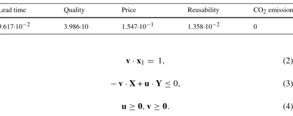
Table 1Solution of the DEA model with reciprocal data for the first supplier

Lead time Quality Price Reusability CO2emission

9.617·10⁻² 3.986·10 1.547·10⁻¹ 1.358·10⁻² 0

v·x1 1, (2)

−v·X+u·Y≤0, (3)

u≥0,v≥0. (4)

Model types (1)–(4) can be solved with commercial software such as Microsoft Excel Solver. Throughout the paper we apply this software to construct our numerical examples (see Table1). Our example fulfils the general rule for the number of decision-making units with regard to valid outcomes. The number of suppliers is equal to 15—i.e.rmax{m·n; 3·(m+n)}, whereris the number of suppliers and numbers m2, andn3 are the number of outputs and inputs (Cooper et al.2001).

The cross-efficiencies of the model (1)–(4) can be calculated for alljmodels, where valuejis the number of a decision-making unit (DMU). Let us assume that the optimal weights (u¹;v¹) of problems (1)–(4) are known. Then the cross-efficiencies for these weights and Supplier 1 are

Ej1u¹·yj/v¹·xj; j 1,2, . . . ,r. (5) The efficiency ofself-appraisal, is equal toEjs Ejj (Doyle and Green1994).

Peer-appraisalfor the first DMU is calculated as the average of the cross-efficiencies:

E1p

i1 i1

pEj i

p−1 , j 1,2, . . . ,r. (6)

We hereby complete the introduction to the basic DEA model. The self-appraisal and peer-appraisal indicators for Supplier 1 are shown in Eqs. (5) and (6).

3.2 The application of an additive DEA model in supplier selection

After introducing “lack of” type variables, the input and output vectors of the suppliers can be summarized in matricesXandY. Let us formulate the additive DEA model in the next format, assuming that we are examining the efficiency of the first decision- making unit:

−ε·1·s⁻−ε·1·s⁺ →min (7) s.t.

(6)

−X·λ−s⁻ −x1 (8)

Y·λ−s⁺ y1 (9)

1·λ1 (10)

λ≥0, s⁻≥0, s⁺ ≥0. (11) Model (7)–(11) is the basic dual model for the additive DEA method which can be reformulated in a primal model in the following form

−v·x1+u·y₁+ u1→max (12) s.t.

−v·X+u·Y+ u1·1≤0 (13)

u≥ε·1,v≥ε·1. (14) The self-appraisal and peer-appraisal indexes of the additive DEA model can be determined in a similar way to that of Eqs. (5) and (6).

4 Numerical examples

Examples of numerical data are presented in “Appendix 1”. Based on these, we first determine the values of self-appraisal and peer-appraisal with the data obtained by reciprocal transformation. Then we transform the data with the additive model. Sec- tion4.3compares the results of self- and peer-appraisal indicators for reciprocal and additive models.

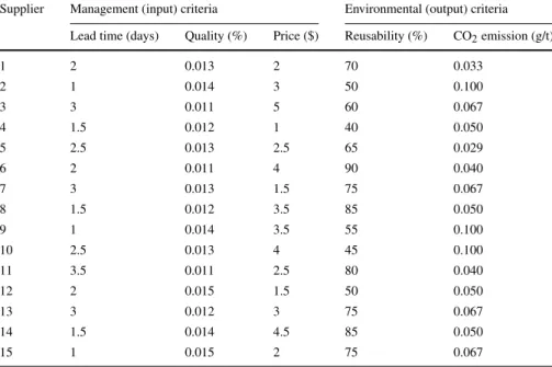
4.1 A DEA model with reciprocal data for supplier selection

Let us transform the data in “Appendix 1” into a form that better fits maximization criterion; i.e., gives higher values than those of a less good evaluation. If a better evaluation produces a higher value, then the evaluation of that criterion shall not be changed. (This is the case, for example, for reusability, lead time, and price.) If a better criterion is awarded a lower value, then we use the inverse (i.e. reciprocals of the data).

The data used for this type of analysis are shown in “Appendix 2”.

The linear programming model gives the following weights for solving the problem for the first supplier. For problems (1)–(4), the optimal weights are given in Table1.

The DEA efficiency measures for the first supplier are shown in the first column of Table2. The other columns in the matrix present the relevant DEA efficiency of the supplier and the cross-efficiencies.

(7)

Table2DEA-efficienciesandCross-efficienciesforDEAmodelwithreciprocaldata 123456789101112131415 10.9510.3890.6370.4060.9510.9470.8400.9510.1670.3970.8440.7000.6710.6630.840 20.6011.0000.9560.8620.6010.5950.4620.6011.0001.0000.4950.6690.8980.6910.462 30.5420.3590.9730.3860.5420.5480.3130.5420.2220.7200.5900.3410.9550.4290.313 40.7081.0000.6621.0000.7080.6980.8730.7080.3330.6740.5691.0000.6440.4710.873 50.7620.2670.5360.2890.7620.7610.6240.7620.1140.3120.7090.5110.5680.5140.624 60.9930.2800.9440.2840.9931.0000.6000.9930.2000.4781.0000.4921.0000.8930.600 71.0000.7780.9411.0001.0001.0001.0001.0000.2220.8210.9551.0000.9410.5241.000 81.0000.4120.9060.3931.0001.0000.6581.0000.3330.5680.9230.5780.9381.0000.658 90.6190.8750.9780.7610.6190.6150.4400.6191.0000.9730.5220.6050.9250.7600.440 100.4400.6671.0000.6880.4400.4410.2920.4400.4001.0000.4300.4490.9330.3560.292 110.9320.3290.8370.4190.9320.9400.7110.9320.1140.5081.0000.5990.8780.5040.711 120.6550.7000.5480.7010.6550.6470.7500.6550.2500.5100.5340.7840.5420.4440.750 130.8340.5191.0000.5960.8340.8400.6000.8340.2220.7820.8540.6001.0000.5300.600 140.8190.3330.7460.3080.8190.8180.5230.8190.3330.4620.7450.4600.7730.9330.523 151.0000.9330.7650.7681.0000.9831.0001.0000.6670.6610.7651.0000.7651.0001.000

(8)

The most DEA efficient and cross-efficient decision-making units with maximal values of one are suppliers 7, 8, and 15. The first supplier in our case has an efficiency score (i.e. self-appraisal) of 0.951, which is relatively high.

In this numerical example, two sets of criteria were formulated: management as input (traditional purchasing) criteria, and environmental, or output criteria.

The weights vector suggests that the weight of all classical purchasing criteria should be incorporated into the evaluation of suppliers. The criterion of reusability received a weight in the analysis, but the criterion of CO2emissions was not evaluated in this model.

The efficiency of each supplier is the solution of problem (1)–(4) by optimizing the values for their own criteria. In the present case we have to solve 15 linear programming problems. When solving certain problems, cross-efficiencies are incidental; that is, with optimal weights the efficiency of other suppliers can be determined.

Table2contains the DEA efficiencies and cross-efficiencies for all suppliers. The diagonal of the matrix shows the DEA efficiencies, which are colored gray. The white elements of the vertical columns include the 14 cross-efficiencies with the optimum weights for the particular supplier.

Table5includes the self- and peer-appraisal values of suppliers. Suppliers 2, 4, 6, 7, 8, 9, 10, 11, 13, and 15 have the highest efficiency, i.e., one. These suppliers are also Pareto efficient, meaning there is no other supplier that outperforms them. However, the remaining five suppliers are inefficient. The cross-efficiencies of suppliers 7, and 15 are around 0.8, or greater. As the purpose of supplier evaluation is to help with selecting a supplier, one should be chosen that clearly has high cross-efficiency and DEA efficiency. In this case, Supplier 10 is efficient, but in terms of peer-appraisal it is weak.

This completes the analysis.

4.2 An additive DEA model in supplier selection

Let us now transform the data from “Appendix 1” for the additive model. If a better evaluation has a higher value, than we will not change the evaluation of that criterion.

If a lower value for a criterion is better, then we will reduce the value of the maximum available quality (i.e. 100 percent) by the supplier’s value for quality, while for CO2

emissions 40 g/t is the least best value, representing the highest CO2 emission of any supplier in this sector. These two upper bounds can be interpreted as “lack of”

parameters. Quality has an upper bound of 100 percent, and we assume an “industrial worst” technology with 40 g/t CO2emissions. The data used for the analysis are shown in “Appendix 3”.

The linear programming model (12)–(14) offers the following weights for solving the problem for the first supplier. These are presented in Table3. Theεvalue for this model is 10⁻⁵. The DEA efficiency measures are shown in the first column of Table4.

The other columns in the matrix present the relevant DEA efficiency of the supplier and the cross-efficiencies as well.

The weights vector suggests that the weight of all classical purchasing features should be incorporated into the evaluation of suppliers. Reusability and CO2emissions

(9)

Table 3Solution of the DEA model for the first supplier

Lead time Quality Price Reusability CO2emission Slack variable (u1) 1.56·10⁻⁴ 1.492·10⁻⁵ 1.8·10⁻⁴ 10⁻⁵ 10⁻⁵ 3.92·10⁻⁵

receive a weight in the analysis as well. The weighting of the environmental criteria is exactly the minimum possible (i.e. 10⁻⁵). This means that these weights are effective in the sense that they take on the lowest possible value.

The most efficient decision-making units with values of over 0.9 are suppliers 4, 6, 7, 8 and 15. The first supplier in our case has an efficiency score of 0.823, which is relatively high.

Analysis from the literature suggests that overall performance can be mapped according to vendor evaluation criteria, such that each of the evaluation criteria is an important company parameter. It is often unacceptable for a company to have a supplier who only fulfils a single criterion well (even if they are extremely good in this regard). According to the literature, such a situation is the result of a utility-maximizing supplier.

The analysis of additive model is complete.

4.3 Comparison of self- and peer-appraisal indicators for reciprocal and additive DEA models

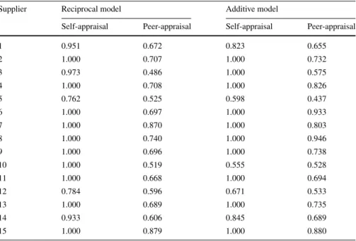
DEA efficiency is relatively easy to interpret. However, there are several interpretations of cross-efficiency (Doyle and Green1994) One interpretation is that DEA efficiency can involve self-appraisal, meaning that the supplier tries to maximize their own efficiency. Cross-efficiencies, on the other hand, develop throughpeer-appraisal. Of course, cross-efficiency is always less than DEA efficiency. The method of calculation of peer-appraisal indexes is shown in (6). Table5summarizes the self-appraisal and peer-appraisal of reciprocal and additive models.

Reciprocal and additive models are compared using a correlation coefficient. First, we discuss the relationship between self-appraisal and peer-appraisal in reciprocal and additive models. In the reciprocal model, the correlation between the two efficiency measures is 0.479. This suggests that there is only a moderate relationship between the two metrics, so DEA efficiency reassesses the value obtained for efficiency using peer-appraisal. In the additive model, the correlation is 0.776, which indicates strong correlation. This shows that the self-appraisal and peer-appraisal metrics are similar.

The correlation coefficient between the two models’ self-appraisal indices is 0.698.

This suggests that if there is a difference between the two models, it is irrelevant.

The correlation between the two peer-appraisal metrics is 0.789. Interestingly, the relationship between peer-appraisal metrics is stronger than that between self-appraisal metrics.

In summarizing the results, we can state that the results obtained by the two data processing methods give almost similar results. Only a significant difference between the two efficiency indicators for the reciprocal model can be identified. This also means that the results are less dependent on data transformation.

(10)

Table4DEA-efficienciesandcross-efficienciesforadditiveDEAmodel 123456789101112131415 10.8230.5640.4020.8270.8550.5830.8480.5830.5380.8270.7570.7780.4420.5830.583 20.6991.0000.7090.7600.7260.6870.7090.6870.9650.7600.5360.6360.6850.8430.843 30.5590.6311.0000.6000.5800.5240.5890.5240.5300.6000.5900.4510.9450.4630.463 40.9390.8611.0001.0000.9750.5850.9660.5850.6751.0000.8690.9441.0000.5850.585 50.5760.3470.1850.5690.5980.4080.5940.4080.3520.5690.5300.5440.2220.4080.408 60.9470.8681.0000.9740.9821.0001.0001.0000.8470.9741.0000.7391.0000.8670.867 70.9620.7070.9371.0001.0000.5511.0000.5510.5591.0001.0000.9660.9670.5200.520 80.9641.0000.8031.0001.0001.0001.0001.0001.0001.0000.8730.7990.8061.0001.000 90.6881.0000.6910.7460.7150.7270.7000.7271.0000.7460.5320.6100.6670.8910.891 100.5050.6490.7510.5550.5240.4330.5220.4330.5330.5550.4610.4430.7180.4330.433 110.8270.5360.8670.8430.8590.5220.8750.5220.4500.8431.0000.7430.9210.4550.455 120.6330.5680.4610.6620.6580.4090.6410.4090.4850.6620.5110.6710.4670.4520.452 130.8100.7041.0000.8500.8410.5830.8480.5830.5780.8500.8560.7181.0000.5320.532 140.7030.7630.4630.7270.7300.7480.7210.7480.8210.7270.5760.6050.4700.8450.845 150.9621.0000.5721.0001.0000.7880.9660.7881.0001.0000.7000.9660.5791.0001.000

(11)

Table 5Efficiency measures of the suppliers

Supplier Reciprocal model Additive model

Self-appraisal Peer-appraisal Self-appraisal Peer-appraisal

1 0.951 0.672 0.823 0.655

2 1.000 0.707 1.000 0.732

3 0.973 0.486 1.000 0.575

4 1.000 0.708 1.000 0.826

5 0.762 0.525 0.598 0.437

6 1.000 0.697 1.000 0.933

7 1.000 0.870 1.000 0.803

8 1.000 0.740 1.000 0.946

9 1.000 0.696 1.000 0.738

10 1.000 0.519 0.555 0.528

11 1.000 0.668 1.000 0.694

12 0.784 0.596 0.671 0.533

13 1.000 0.689 1.000 0.735

14 0.933 0.606 0.845 0.689

15 1.000 0.879 1.000 0.880

5 Conclusion

In this paper, a cross-efficiency DEA model was defined. The proposed model addresses two problems. First, we provide an example of supplier evaluation using negative data. In classical DEA models, input and output data cannot be transformed together, so data translation must be undertaken. Therefore, additive DEA models are almost exclusively used to deal with such problems.

Second, the method should respond to modifications in suppliers’ offers in the case that a buyer favors overall good performance. To filter suppliers with data outliers in supplier evaluation, it is important to distinguish between self-appraisal and peer- appraisal. Self-appraisal metrics cover DEA efficiency, while peer-appraisal indicators cover cross-efficiency. In traditional DEA models it is possible to filter out efficient suppliers based on self-appraisal. Moreover, by applying the concept of cross-efficiency it is possible to differentiate between generally good performance and partially good performance with the help of peer-appraisal.

Finally, reciprocal and additive model self- and peer-appraisal indicators were compared. The correlation analysis showed a very strong linear relationship in terms of the efficiency of the two DEA models in our numerical example. The conditions under which the efficiency measures applied in the two models differ should be further investigated.

Cross-efficiency is rarely used in an additive model. In additive DEA models, efficiency can be greater than one. The numerical example presented here indicates that all self-appraisal DEA and aggregate peer-appraisal cross-efficiency values can be between zero and one.

(12)

The role of weights may also be the subject of future study.

Acknowledgements Open access funding provided by Corvinus University of Budapest (BCE). This research project was supported by NKFIH. (Project No. K 124644).

Open Access This article is licensed under a Creative Commons Attribution 4.0 International License, which permits use, sharing, adaptation, distribution and reproduction in any medium or format, as long as you give appropriate credit to the original author(s) and the source, provide a link to the Creative Commons licence, and indicate if changes were made. The images or other third party material in this article are included in the article’s Creative Commons licence, unless indicated otherwise in a credit line to the material. If material is not included in the article’s Creative Commons licence and your intended use is not permitted by statutory regulation or exceeds the permitted use, you will need to obtain permission directly from the copyright holder. To view a copy of this licence, visithttp://creativecommons.org/licenses/by/4.0/.

Appendix 1 See Table6.

Table 6Data for numerical examples

Supplier Management (input) criteria Environmental (output) criteria Lead time (days) Quality (%) Price ($) Reusability (%) CO2 emission (g/t)

1 2 80 2 70 30

2 1 70 3 50 10

3 3 90 5 60 15

4 1.5 85 1 40 20

5 2.5 75 2.5 65 35

6 2 95 4 90 25

7 3 80 1.5 75 15

8 1.5 85 3.5 85 20

9 1 70 3.5 55 10

10 2.5 75 4 45 10

11 3.5 90 2.5 80 25

12 2 65 1.5 50 20

13 3 85 3 75 15

14 1.5 70 4.5 85 20

15 1 65 2 75 15

(13)

Table 7Data for DEA model with reciprocal data

Supplier Management (input) criteria Environmental (output) criteria Lead time (days) Quality (%) Price ($) Reusability (%) CO2emission (g/t)

1 2 0.013 2 70 0.033

2 1 0.014 3 50 0.100

3 3 0.011 5 60 0.067

4 1.5 0.012 1 40 0.050

5 2.5 0.013 2.5 65 0.029

6 2 0.011 4 90 0.040

7 3 0.013 1.5 75 0.067

8 1.5 0.012 3.5 85 0.050

9 1 0.014 3.5 55 0.100

10 2.5 0.013 4 45 0.100

11 3.5 0.011 2.5 80 0.040

12 2 0.015 1.5 50 0.050

13 3 0.012 3 75 0.067

14 1.5 0.014 4.5 85 0.050

15 1 0.015 2 75 0.067

(14)

Table 8The translated data for additive model

Supplier Management (input) criteria Environmental (output) criteria Lead time (days) Quality (%) Price ($) Reusability (%) CO2emission (g/t)

1 2 20 2 70 10

2 1 30 3 50 30

3 3 10 5 60 25

4 1.5 15 1 40 20

5 2.5 25 2.5 65 5

6 2 5 4 90 15

7 3 20 1.5 75 25

8 1.5 15 3.5 85 20

9 1 30 3.5 55 30

10 2.5 25 4 45 30

11 3.5 10 2.5 80 15

12 2 35 1.5 50 20

13 3 15 3 75 25

14 1.5 30 4.5 85 20

15 1 35 2 75 25

(15)

References

Agarwal P, Sahai M, Mishra V, Bag M, Singh V (2011) A review of multi-criteria decision making techniques for supplier evaluation and selection. Int J Ind Eng Comput 2(4):801–810.https://doi.org/10.5267/j.

ijiec.2010.06.004

Bai C, Sarkis J (2016) Supplier development investment strategies: a game theoretic evaluation. Ann Oper Res 240(2):583–615.https://doi.org/10.1007/s10479-014-1737-9

Bruno G, Esposito E, Genovese A, Passaro R (2012) AHP-based approaches for supplier evaluation: problems and perspectives. J Purch Supply Manag 18(3):159–172.https://doi.org/10.1016/j.pursup.2012.

05.001

Chai J, Liu JN, Ngai EW (2013) Application of decision-making techniques in supplier selection: a systematic review of literature. Expert Syst Appl 40(10):3872–3885.https://doi.org/10.1016/j.eswa.201 2.12.040

Charnes A, Cooper WW, Rhodes E (1978) Measuring the efficiency of decision making units. Eur J Oper Res 2(6):429–444.https://doi.org/10.1016/0377-2217(78)90138-8

Cook WD, Seiford LM (2009) Data envelopment analysis (DEA)–thirty years on. Eur J Oper Res 192(1):1–17.https://doi.org/10.1016/j.ejor.2008.01.032

Cooper WW, Li S, Seiford LM, Tone K, Thrall RM, Zhou J (2001) Sensitivity and stability analysis in DEA: some recent developments. J Prod Anal 15:217–246.https://doi.org/10.1023/A:101112840925 7

De Boer L, Labro E, Morlacchi P (2001) A review of methods supporting supplier selection. Eur J Purch Supply Manag 7(2):75–89.https://doi.org/10.1016/S0969-7012(00)00028-9

Dobos I, Vörösmarty G (2014) Green supplier selection and evaluation using DEA-type composite indicators. Int J Prod Econ 157:273–278.https://doi.org/10.1016/j.ijpe.2014.09.026

Dobos I, Vörösmarty G (2019a) Inventory-related costs in green supplier selection problems with Data Envelopment Analysis (DEA). Int J Prod Econ 209:374–380.https://doi.org/10.1016/j.ijpe.2018.03.0 22

Dobos I, Vörösmarty G (2019b) Evaluating green suppliers: improving supplier performance with DEA in the presence of incomplete data. CEJOR 27(2):483–495.https://doi.org/10.1007/s10100-018-0544-9 Doyle J, Green R (1994) Efficiency and cross-efficiency in DEA: derivations, meanings and uses. J Oper

Res Soc 45(5):567–578.https://doi.org/10.1057/jors.1994.84

Ebrahimi B, Tavana M, Rahmani M, Santos-Arteaga FJ (2018) Efficiency measurement in data envelopment analysis in the presence of ordinal and interval data. Neural Comput Appl 30(6):1971–1982.https://

doi.org/10.1007/s00521-016-2826-2

Foerstl K, Hartmann E, Wynstra F, Moser R (2013) Cross-functional integration and functional coordination in purchasing and supply management: antecedents and effects on purchasing and firm performance.

Int J Oper Prod Manag 33(6):689–721.https://doi.org/10.1108/IJOPM-09-2011-0349

Govindan K, Rajendran S, Sarkis J, Murugesan P (2015) Multi criteria decision making approaches for green supplier evaluation and selection: a literature review. J Clean Prod 98:66–83.https://doi.org/10.

1016/j.jclepro.2013.06.046

Hartmann E, Kerkfeld D, Henke M (2012) Top and bottom line relevance of purchasing and supply management. J Purch Supply Manag 18(1):22–34.https://doi.org/10.1016/j.pursup.2011.12.001 Ho W, Xu X, Dey PK (2010) Multi-criteria decision making approaches for supplier evaluation and selection:

a literature review. Eur J Oper Res 202(1):16–24.https://doi.org/10.1016/j.pursup.2011.12.001 Hong GH, Park SC, Jang DS, Rho HM (2005) An effective supplier selection method for constructing a

competitive supply-relationship. Expert Syst Appl 28(4):629–639.https://doi.org/10.1016/j.eswa.20 04.12.020

Izadikhah M, Saen RF (2016) Evaluating sustainability of supply chains by two-stage range directional measure in the presence of negative data. Transp Res Part D Transp Environ 49:110–126.https://doi.

org/10.1016/j.trd.2016.09.003

Janda S, Seshadri S (2001) The influence of purchasing strategies on performance. J Bus Ind Market 16(4):294–308.https://doi.org/10.1108/EUM0000000005502

Ji P, Ma X, Li G (2015) Developing green purchasing relationships for the manufacturing industry: an evolutionary game theory perspective. Int J Prod Econ 166:155–162.https://doi.org/10.1016/j.ijpe.20 14.10.009

(16)

Kleinsorge IK, Schary PB, Tanner RD (1992) Data envelopment analysis for monitoring customer-supplier relationships. J Account Public Policy 11(4):357–372.https://doi.org/10.1016/0278-4254(92)90004- H

Lovell CK, Pastor JT (1995) Units invariant and translation invariant DEA models. Oper Res Lett 18(3):147–151.https://doi.org/10.1016/0167-6377(95)00044-5

Martos B (1964) Hyperbolic programming. Naval Res Logist Q 11(2):135–155.https://doi.org/10.1002/

nav.3800110204

Mohammaditabar D, Ghodsypour SH, Hafezalkotob A (2016) A game theoretic analysis in capacity- constrained supplier-selection and cooperation by considering the total supply chain inventory costs.

Int J Prod Econ 181:87–97.https://doi.org/10.1016/j.ijpe.2015.11.016

Nerali´c L, Wendell RE (2019) Sensitivity in DEA: an algorithmic approach. CEJOR 27(4):1245–1264.

https://doi.org/10.1007/s10100-018-0587-y

Pastor, JT, Ruiz, JL (2007) Variables with negative values in DEA. In: Modeling data irregularities and structural complexities in data envelopment analysis. Springer, Boston, MA, pp 63–84.https://doi.

org/10.1007/978-0-387-71607-7_4

Prajogo D, Chowdhury M, Yeung AC, Cheng TCE (2012) The relationship between supplier management and firm’s operational performance: a multi-dimensional perspective. Int J Prod Econ 136(1):123–130.

https://doi.org/10.1016/j.ijpe.2011.09.022

Saen RF (2007) Suppliers selection in the presence of both cardinal and ordinal data. Eur J Oper Res 183(2):741–747.https://doi.org/10.1016/j.ejor.2006.10.022

¸Sen CG, ¸Sen S, Ba¸slıgil H (2010) Pre-selection of suppliers through an integrated fuzzy analytic hierarchy process and max-min methodology. Int J Prod Res 48(6):1603–1625.https://doi.org/10.1080/002075 40802577946

Tchokogué A, Nollet J, Robineau J (2017) Supply’s strategic contribution: an empirical reality. J Purch Supply Manag 23(2):105–122.https://doi.org/10.1016/j.pursup.2016.07.003

Toloo M, Nalchigar S, Sohrabi B (2018) Selecting most efficient information system projects in presence of user subjective opinions: a DEA approach. CEJOR 26(4):1027–1051.https://doi.org/10.1007/s10 100-018-0549-4

Vörösmarty G, Dobos I (2019) Supplier evaluation with environmental aspects and common DEA weights.

Periodica Polytech Soc Manag Sci 27(1):17–25.https://doi.org/10.3311/PPso.11814

Wetzstein A, Feisel E, Hartmann E, Benton WC Jr (2018) Uncovering the supplier selection knowledge structure: a systematic citation network analysis from 1991 to 2017. J Purch Supply Manag.https://

doi.org/10.1016/j.pursup.2018.10.002

Publisher’s Note Springer Nature remains neutral with regard to jurisdictional claims in published maps and institutional affiliations.