Introduction to data analysis

(1)

Introduction to data analysis

Borbála Szüle

Corvinus University of Budapest

(2)

SPSS^R is a registered trademark of International Business Machines (IBM) Corporation

ISBN: 978-963-503-619-6

Publisher: Budapesti Corvinus Egyetem, Közgazdaságtudományi Kar (Corvinus University of Budapest, Faculty of Economics)

2016

(3)

(4)

Preface

With the latest development in computer science, multivariate data analysis methods became increasingly popular among economists. Pattern recog- nition in complex economic data and empirical model construction can be more straightforward with proper application of modern softwares. However, despite the appealing simplicity of some popular software packages, the interpretation of data analysis results requires strong theoretical knowledge. This book aims at combining the development of both theoretical and application- related data analysis knowledge. The text is designed for advanced level studies and assumes acquaintance with elementary statistical terms. After a brief introduction to selected mathematical concepts, the highlighting of selected model features is followed by a practice-oriented introduction to the interpretation of SPSS¹ outputs for the described data analysis methods.

Learning of data analysis is usually time-consuming and requires efforts, but with tenacity the learning process can bring about a significant improvement of individual data analysis skills.

1IBM Corp. Released 2013. IBM SPSS Statistics for Windows, Version 22.0. Armonk, NY: IBM Corp.

i

(7)

(8)

1 | Introduction to mathematics

1.1 Matrix calculations

Matrix calculations are often applied in data analysis. The number of rows and columns of a matrix may differ. If the number of rows and columns are equal, the matrix is called a square matrix. Square matrices are not necessarily symmetric matrices (that are symmetric about the diagonal¹).

For a matrix M the transposed matrix is denoted by M^T. The rows of the transposed matrix M^T correspond to the columns of M (and the columns of M^T correspond to the rows of M). If M is a symmetric matrix, then M =M^T.

An identity matrix (of order n) is a square matrix with n rows and columns having ones along the diagonal and zero values elsewhere. If the identity matrix is denoted by I, then the relationship of a square matrix M and the inverse of M (denoted by M⁻¹) is as follows (Sydsæter-Hammond (2008), page 591):

M M⁻¹ =M⁻¹M =I (1.1)

In some cases the determinant of a matrix should be interpreted in data analysis. The determinant of a matrix is a number that can be calculated based on the matrix elements. Determinant calculation is relatively simple in case of a matrix that has two rows and columns. For example assume that a matrix is defined as follows:

M =

m₁₁ m₁₂ m21 m22

(1.2) For the matrixM the determinant can be calculated according toSydsæter- Hammond (2008), (page 574):

1In this case the diagonal of a square matrix with ncolumns is defined as containing the elements in the intersection of the i-th row andi-th column of the matrix (i=1, . . . , n).

1

(9)

2 CHAPTER 1. INTRODUCTION TO MATHEMATICS

det(M) =m₁₁m₂₂−m₁₂m₂₁ (1.3) In this example the determinant occurs also in the calculation of the inverse matrix. The inverse of matrix M in this example can be calculated as follows (Sydsæter-Hammond (2008), page 593):

M⁻¹ = 1 det(M)

m₂₂ −m₁₂

−m₂₁ m₁₁

(1.4)

If for example M1 =

1 0.8 0.8 1

, then det(M1) = 1−0.8² = 0.36. The determinant of the identity matrix is equal to one. If all elements in a row (or column) of a matrix are zero, then the determinant of the matrix is zero. (Sydsæter-Hammond (2008), page 583) If the determinant of a square matrix is equal to zero, then the matrix is said to be singular. A matrix has an inverse if and only if it is nonsingular. (Sydsæter-Hammond (2008), page 592)

The determinant can be interpreted in several ways, for example a ge- ometric interpretation for det(M₁) is illustrated by Figure 1.1, where the absolute value of the determinant is equal to the area of the parallelogram.

(Sydsæter-Hammond(2008), page 575)

Figure 1.1: Matrix determinant

In data analysis it is sometimes necessary to calculate the determinant of a correlation matrix. If the variables in the analysis are (pairwise) uncorrelated, then the correlation matrix is the identity matrix, and in this case the determinant of the correlation matrix is equal to one. If however

(10)

1.1. MATRIX CALCULATIONS 3 the variables in an analysis are “perfectly” correlated so that the (pairwise) correlations are all equal to one, then the determinant of the correlation matrix is equal to zero. In this case (if the determinant is equal to zero) the correlation matrix is singular and does not have an inverse.

For a square matrix M a scalar λ (called „eigenvalue”) and a nonzero vector x(called „eigenvector”) can be found such that (Rencher-Christensen (2012), page 43)

M x=λx (1.5)

If matrixM has nrows andn columns, then the number of eigenvalues is n, but these eigenvalues are not necessarily nonzero. Eigenvectors are unique only up to multiplication by a value (scalar). (Rencher-Chriszensen (2012), page 42) The eigenvalues of a positive semidefinite matrix M are positive or zero values, where the number of positive eigenvalues is equal to the rank of the matrix M. (Rencher-Christensen (2012), page 44) The eigenvectors of a symmetric matrix are mutually orthogonal. (Rencher-Christensen (2012), page 44)

According to the spectral decomposition theorem for each symmetric ma- trixM an orthonormal basis containing the eigenvectors of matrix M exists so that in this basisM is diagonal:

D=B^TM B (1.6)

where D is a diagonal matrix and the diagonal values are the eigenvalues of M (Medvegyev (2002), page 454). In case of this orthonormal basis B^T = B⁻¹, which means that the transpose matrix and the inverse matrix are identical. (Medvegyev (2002), page 454) According to the spectral decomposition theorem, the symmetric matrixM can be expressed in terms of its eigenvalues and eigenvectors (Rencher-Christensen (2012), page 44):

M =BDB^T (1.7)

Assume that the (real) matrix X has nrows and pcolumns and the rank of matrix X is equal to k. In this case the singular value decomposition of matrixX can be expressed as follows (Rencher-Christensen(2012), page 45):

X =U DV^T (1.8)

where matrix U has n rows and k columns, the diagonal matrix D has k rows and k columns and matrix V has p rows and k columns. In this case the diagonal elements of the (non-singular) diagonal matrix D are the positive square roots of the nonzero eigenvalues of X^TX or of XX^T. The

(11)

4 CHAPTER 1. INTRODUCTION TO MATHEMATICS diagonal elements of matrix D are called the singular values of matrix X.

The columns of matrix V are the normalized eigenvectors of X^TX and the columns of matrix U are the normalized eigenvectors of XX^T. (Rencher- Christensen (2012), page 45)

A positive semidefinite matrixM can be expressed also as follows (Rencher- Christensen (2012), page 38):

M =A^TA (1.9)

where A is a nonsingular upper triangular matrix that can be calculated for example with Cholesky decomposition. Calculation details about Cholesky decomposition can be found for example in Rencher-Christensen (2012) (on pages 38-39).

1.2 Probability theory

Data analysis is usually based on (randomly selected) statistical samples.

Theoretically, statistical sampling may contribute to answer quantitative re- search questions, since according to the Glivenko-Cantelli theorem, as the number of independent and identically distributed sample observations increases, the empirical distribution function (belonging to the sample) almost surely converges to the theoretical (population) distribution function. (Med- vegyev(2002), page 542). This theorem is one of the theoretical reasons why data analysis is often related to probability theory. For instance, confidence intervals and empirical significance levels (“p-values”) are usually calculated with assuming (theoretically explainable) probability distributions in case of certain variables.

The normal distribution is among the most frequently applied probability distributions in data analysis. In the univariate case it has two parameters (µ and σ, indicating the mean and the standard deviation, respectively). The probability density function is:

f(x) = 1 σ√

2πe⁻^(x−µ)2^2σ (1.10)

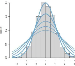
for −∞< x <∞ where −∞< µ < ∞ and σ >0. (David et al. (2009), page 465). This density function (for different standard deviations and with the mean being equal to zero) is illustrated by Figure 1.2. The histogram on Figure 1.2 belongs to a standard normal distribution (simulated data with a sample size of 1000). On Figure 1.2, the blue lines indicate the theoretical density functions belonging to the normal distributions with the standard

(12)

1.2. PROBABILITY THEORY 5 deviation values 1, 1.25, 1.5, 1.75 and 2, respectively (and with a theoretical mean which is equal to zero for each blue line on Figure 1.2).

Figure 1.2: Normal distributions

Some probability distributions are related to the normal distribution. The chi-squared distribution is the sum of n independent random variables that are the squares of standard normally distributed random variables: if ξ₁, ξ₂, . . .ξ_nare (independent) random variables with standard normal distribution, then the distribution of the random variable is called χ²-distribution with n degrees of freedom. The mean of the χ²-distribution with n degrees of freedom isn, the variance is2n. (Medvegyev(2002), pages 263-264) Figure 1.3 illustrates χ²-distributions with different degrees of freedom. The histogram on Figure 1.3 belongs to a χ²₂ distribution (simulated data with a sample size of 1000), and the blue lines indicate the theoretical density functions belonging to χ²₂, . . . , χ²₁₁ distributions. It can be observed on Figure 1.3, that for higher degrees of freedom the density function of the χ² distribution becomes more symmetric.

Probability theory distinguishes univariate distributions from multivariate distributions (that are defined for a vector of random variables. If for example ξ₁, . . . ξ_m are random variables, then the (ξ₁, . . . , ξ_m) variable (the vector of the ξ1, . . . ξm random variables) has a multivariate normal distribution, if for eacht_i (i= 1, . . . , m) real numbers the distribution of the

(13)

Figure 1.3: Chi-squared distributions

following random variable is a normal distribution (Medvegyev (2002), page 453):

m

X

i=1

t_iξ_i (1.11)

A multivariate normal distribution has a mean vector (instead of only one number as the mean of the distribution) and a covariance matrix (instead of one number as the variance of the distribution). The covariance matrix of a multivariate normal distribution is a positive semidefinite matrix (Medvegyev (2002), page 453).

Assume in the following that the covariance matrix of a multivariate normal distribution is denoted by C and also assume that matrix C has m rows and m columns. In that case if the rank of C is r, then matrix A (that has m rows and r columns) exists so that C = AA^T. This result is a consequense of the spectral decomposition theorem. (Medvegyev (2002), page 454)

According to the spectral decomposition theorem for each symmetric ma- trixM an orthonormal basis containing the eigenvectors of matrixM exists so that in this basisM is diagonal:

(14)

1.2. PROBABILITY THEORY 7

(a)ρ=0.8 (b)ρ=0

(c)ρ=-0.9

Figure 1.4: Multivariate normal distributions

D=B^TM B (1.12)

whereD is a diagonal matrix and the diagonal values are the eigenvalues of M (Medvegyev (2002), page 454). It is worth mentioning that in case of this orthonormal basis B^T =B⁻¹, which means that the transposed matrix and the inverse matrix are identical. (Medvegyev (2002), page 454)

In case of a multivariate normal distribution the covariance matrix contains information about the independence of the univariate random variables.

However it is worth emphasizing that the covariance (and thus correlation coefficient) can not automatically be applied to test whether two random variables are independent: uncorrelated random variables can only then be considered as independent if the joint distribution of the variables is a multivariate normal distribution. (Medvegyev (2002), page 457)

Figure 1.4 illustrates density functions of multivariate normal distribu-

(15)

(a)ρ=0.8 (b)ρ=0

(c)ρ=-0.9

Figure 1.5: Effect of correlation

tions with different theoretical correlations coefficient (indicated by ρ). It can be observed on Figure 1.4 that as the absolute value of the theoretical correlation coefficient increases, the area on the density function graph, where the density function value is not close to zero, becomes smaller. The same phenomenon can be observed on Figure 1.5, which shows simulated data on scatter plots that belong to the cases ρ = 0.8, ρ= 0 and ρ=−0.9, respectively (with the assumption that the univariate distributions belonging to the simulations are normal distributions). The effect of a change of sign belonging to the theoretical correlation can also be observed on Figure 1.4 and Figure 1.5.

(16)

2 | Cluster analysis

Cluster models are usually used to find groups (clusters) of similar records based on the variables in the analysis, where the similarity between members of the same group is high and the similarity between members of different groups is low. With cluster analysis it may be possible to identify relatively homogeneous groups (“clusters”) of observations. There are several cluster analysis methods, in this chapter selected features of hierarchical, k-means and two-step clustering are introduced.

2.1 Theoretical background

Hierarchical, k-means and two-step cluster analysis apply different algorithms for creating clusters. The hierarchical cluster analysis procedure is usually limited to smaller data files (for example in case of thousands of objects the application of this analysis is usually related to significant computational cost). The k-means cluster analysis procedure and two-step clustering can be considered as more suitable to analyze large data files.

Theoretically, in case of hierarchical cluster analysis the aggregation from individual points to the most high-level cluster (agglomerative approach, bottom-up process) or the division from a top cluster to atomic data objects (divisive hierarchical clustering, top-down approach) can also be solved from a computational point of view. (Bouguettaya et al. (2015)) In the following selected features of the agglomerative hierarchical clustering are introduced.

As opposed to hierarchical clustering, k-means cluster analysis is related to a partitional clustering algorithm, which repeatedly assigns each object to its closest cluster center and calculates the coordinates of new cluster centers accordingly, until a predefined criterion is met. (Bouguettaya et al. (2015)) In case of two-step clustering procedure it may be possible to pre-cluster the observations into many small subclusters in the first step and group the subclusters into final clusters in the second step. (Steiner-Hudec (2007))

One of the differences between hierarchical and k-means clustering is that 9

(17)

10 CHAPTER 2. CLUSTER ANALYSIS as long as all the variables are of the same type, the hierarchical cluster analysis procedure can analyze both “scale” or “categorical” (for example also binary) variables, but the k-means cluster analysis procedure is basically limited to “scale” variables. In case of two-step clustering it may be possible that “scale” and “categorical” variables can be combined. In cluster analysis, usually the standardization of “scale” variables should be considered. Cluster analysis is usually applied for grouping cases, but clustering of variables (rather than cases) is also possible (in case of hierarchical cluster analysis).

(George–Mallery(2007), page 262)

The algorithm used in (agglomerative) hierarchical cluster analysis starts by assuming that each case (or variable) can be considered as a separate cluster, then the algorithm combines clusters until only one cluster is left. If the number of cases is n, then the number of steps in the analysis is n−1 (it means that after n−1 steps all cases are in one cluster). The distance or similarity measures used in the hierarchical cluster analysis should be appropriate for the variables in the analysis. In case of “scale” variables (and assuming that the value of the jth variable in case of the ith observation is indicated by x_ij), for example the following distance or similarity measures can be used in the analysis (Kovács (2011), page 45):

- Euclidean distance: r P

j

(x_ij −x_kj)²

- squared Euclidean distance: P

j

(x_ij −x_kj)²

- Chebychev method for the calculation of distance: max

j |x_ij −x_kj|² - City-block (Manhattan): P

j

|xij −xkj|² - „customized”: (P

j

|xij −xkj|^p)¹^r

- etc.

The cluster methods in a hierarchical cluster analysis (methods for agglomeration in n−1 steps) can also be chosen, available alternatives are for example (Kovács (2011), pages 47-48):

- nearest neighbor method (single linkage): the distance between two clusters is equal to the smallest distance between any two members in the two clusters

(18)

2.1. THEORETICAL BACKGROUND 11 - furthest neighbor method (complete linkage): the distance between two clusters is equal to the largest distance between any two members in the two clusters

- Ward’s method: clusters are created in such a way to keep the within- cluster „variability” as small as possible

- within-groups linkage - between-groups linkage - centroid clustering - median clustering.

One of the most important graphical outputs of a hierarchical cluster analysis is the dendrogram that displays distance levels at which objects and clusters have been combined.

The k-means cluster analysis is a non-hierarchical cluster analysis method that attempts to identify relatively homogeneous groups of cases in case of a specified number of clusters (this number of clusters is indicated byk). The distances in this analysis are computed based on Euclidean distance. The k- means cluster analysis applies iteration when cases are assigned to clusters.

Iteration in this analysis starts with the selection of initial cluster centers (number of cluster centers is equal to k). Iteration stops when a complete iteration does not move any of the cluster centers by a distance of more than a given value. (Kovács (2014), page 61)

Some important outputs of the k-means cluster analysis:

- final cluster centers

- distances between cluster centers

- ANOVA-table (the F tests are only descriptive in this table) - number of cases in clusters.

The maximum number of clusters is sometimes calculated as p_n

2 (where n indicates the number of observations in the cluster analysis). (Kovács (2014), page 62) There are several methods how to choose the number of clusters in a cluster analysis. For example in addition to the studying of the dendrogram (if it is possible) the “cluster elbow method” can also provide information about the “optimal” number of clusters (Kovács (2014), page 62) The measurement of silhouette can also contribute to the selection of

(19)

12 CHAPTER 2. CLUSTER ANALYSIS an „appropriate” number of clusters (Rousseeuw (1987)). For each object it is possible to define values (for example for the ith observation s(i)) with an absolute value smaller or equal to one (in case of s(i) the minimum can be minus one and the maximum can be one), so that a higher s(i) value indicates a “better” clustering result. The “silhouette” of a cluster can be defined as a plot of s(i) values (ranked in decreasing order). The average of the s(i) values can be calculated and that number of cluster could be considered as “appropriate”, for which the average of the s(i) values is the largest. (Rousseeuw (1987))

2.2 Cluster analysis examples

In the following selected information society indicators (belonging to Eu- ropean Union member countries, for the year 2015) are analyzed: data is downloadable from the homepage of Eurostat¹ and it is also presented in the Appendix. In the following cluster analysis examples are presented with the application of the following three variables:

- “ord”: individuals using the internet for ordering goods or services - “ord_EU”: individuals using the internet for ordering goods or services

from other EU countries

- “enterprise_ord”: enterprises having received orders online.

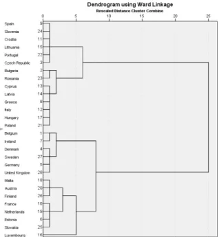
Question 2.1. Conduct hierarchical cluster analyis (with squared Euclidean distance and Ward’s method). Do Spain and Luxembourg belong to the same cluster, if the number of clusters is equal to 2?

Solution of the question.

In case of cluster analysis “scale” variables are usually standardized. Stan- dardization of a variable can be considered as a (relatively) straightforward procedure: the average value is subtracted from the value (for each case sep- arately) and then this difference is divided by the standard deviation. As a result of this calculation, the mean of a standardized variable is equal to zero and the standard deviation is equal to one. Standardized variables can

1Data source: homepage of Eurostat (http://ec.europa.eu/eurostat/web/information- society/data/main-tables)

(20)

2.2. CLUSTER ANALYSIS EXAMPLES 13 be created in SPSS by performing the following sequence (beginning with selecting “Analyze” from the main menu):

Analyze ÝDescriptive Statistics ÝDescriptives...

In this example, in the appearing dialog box the variables “ord”, “ord_EU”

and “enterprise_ord” should be selected as “Variable(s):”, and the option

“Save standardized values as variables” should also be selected. After clicking

“OK” the standardized variables are created.

Figure 2.1: Dendrogram with Ward linkage

To conduct a hierarchical cluster analysis in SPSS perform the following sequence (beginning with selecting “Analyze” from the main menu):

Analyze ÝClassify ÝHierarchical Cluster...

As a next step, in the appearing dialog box select the three standardized variables as “Variable(s):”, and in case of “Method...” button select “Ward’s method” as “Cluster Method:” and “Squared Euclidean distance” as “Mea- sure”. The dendrogram is displayed as an output, if the “Dendrogram” option is selected in case of “Plots...” button.

(21)

14 CHAPTER 2. CLUSTER ANALYSIS The dendrogram is shown by Figure 2.1. It can be observed, that if the number of clusters is equal to 2, then the number of countries in both clusters is equal to 14, and it can also be observed that Spain and Luxembourg do not belong to the same cluster.

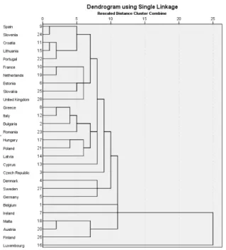
Question 2.2. Conduct hierarchical cluster analyis (with Euclidean distance and nearest neighbor method). How many countries are in the clusters, if the number of clusters is equal to 2?

Figure 2.2: Dendrogram with single linkage

In case of the dialog box (belonging to hierarchical cluster analysis in SPSS) similar options can be selected as for Question 2.1, the only difference is in case of the “Method...” button: to solve Question 2.2 “Nearest neighbor”

should be selected as “Cluster method”, and “Euclidean distance” should be selected as “Measure”.

Figure 2.2 shows the dendrogram (belonging to nearest neighbor method and Euclidean distance). It can be observed on Figure 2.2 that if the number of clusters is equal to 2, then in one of the clusters there is only one country

(22)

2.2. CLUSTER ANALYSIS EXAMPLES 15 (Luxembourg), thus (since the number of countries in the analysis is 28), the number of countries in the clusters are 27 and 1, respectively.

Question 2.3. Conduct hierarchical cluster analyis (with Euclidean distance and nearest neighbor method). Which two countries belong to the first cluster (in the process of agglomeration in hierarchical cluster analysis) that has at least two elements?

Table 2.1: Agglomeration schedule in hierarchical cluster analysis

In this case the same options should be selected in the dialog box (that belongs to hierarchical cluster analysis in SPSS) as in case of Question 2.2.

One of the outputs is the “Agglomeration schedule” that summarizes information about the process of agglomeration in hierarchical cluster analysis.

Table 2.1 shows this “Agglomeration schedule”. It is worth noting that this

“Agglomeration schedule” contains information about 27 steps in the process of agglomeration (since the number of cases in the analysis is equal to 28).

(23)

16 CHAPTER 2. CLUSTER ANALYSIS In the first row of this table it can be observed that the countries indicated by “9” and “24” are in the first cluster that has two elements (before the first step in the agglomeration process each case can be considered to be a cluster that contains one element). Thus, in this example Spain (the country indicated by “9”) and Slovenia (the country that is indicated by “24” in this case) belong to the first cluster that has at least two elements.

Question 2.4. Conduct k-means cluster analyis with k=2. Which variables should be omitted from the analysis?

To conduct a k-means cluster analysis in SPSS perform the following sequence (beginning with selecting “Analyze” from the main menu):

Analyze ÝClassify ÝK-Means Cluster...

As a next step, in the appearing dialog box select the three standardized variables as “Variables:”. As “Number of Clusters:” 2 should be written (it is also the default value) and in case of the “Options...” button select “ANOVA table”.

Table 2.2 shows the ANOVA table that is one of the outputs of the k- means cluster analysis. In the last column of this ANOVA table all values can be considered as relatively small (smaller than 0.05, but in this case these values can not be interpreted exactly in the same way as in case of a

“classical” hypothesis testing, since the results of the presented F tests should only be applied for descriptive purposes). The conclusion is that no variables should be omitted from the analysis in this example.

Table 2.2: ANOVA in k-means cluster analysis

(24)

2.2. CLUSTER ANALYSIS EXAMPLES 17 Question 2.5. Which can be considered as the optimal number of clusters in k-means cluster analysis according to the “cluster elbow” method?

In the following, “cluster elbow” calculations are introduced based on Kovács (2014) (page 62). Since the solution of Question 2.4 indicates that none of the variables should be omitted from the analysis, these three (standardized) variables are applied in k-means cluster analyses (so that the cluster membership variables are saved). The (standardized) variables and the cluster membership variables are applied in one-way ANOVA (the results for k = 2 are shown by Table 2.3).

To conduct one-way ANOVA in SPSS perform the following sequence (beginning with selecting “Analyze” from the main menu):

Analyze Ý Compare Means Ý One-Way ANOVA...

As a next step, in the appearing dialog box select the three standardized variables in case of the “Dependent List:” and the saved cluster membership variable as “Factor”.

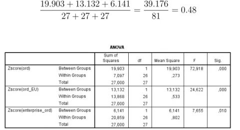
The “cluster elbow” graph (demonstrated by Figure 2.3) plots certain ratios against k values, for example the ratio (plotted on the “cluster elbow”

graph) for k = 2 can be calculated as follows (based on the values in Table 2.3):

19.903 + 13.132 + 6.141

27 + 27 + 27 = 39.176

81 = 0.48 (2.1)

Table 2.3: ANOVA with cluster membership variable

(25)

18 CHAPTER 2. CLUSTER ANALYSIS Figure 2.3 shows the “cluster elbow” graph. According to Kovács (2014) (page 62) the “optimal” number of cluster corresponds to thatk value, where (on the graph) the slope of the graph becomes smaller. In this example it can not be considered as obvious which k corresponds to this requirement.

Both k = 2 and k = 3 could be chosen (k = 4 should not be chosen, since q28

2 <4), thus it could depend on the other features of the analysis, which k is considered as “optimal” (for example the number of cases in the clusters could be compared for the solutions wherek = 2 or k = 3).

Figure 2.3: Cluster elbow method calculation results

Question 2.6. Conduct k-means cluster analysis with k=2. How can the result about the final cluster centers be interpreted?

In this case the same options should be selected in the dialog box (that belongs to hierarchical cluster analysis in SPSS) as in case of Question 2.4.

Table 2.4 contains information about the final cluster centers (in case of k = 2). Since the analysis has been carried out with standardized variables (when the average value of each variable is equal to zero), thus in Table 2.4 positive numbers can be interpreted as “above average” values (and negative numbers refer to “below average” values). For example in case of Cluster 1 all values are above average, and thus the “name” of this cluster (if a “name”

should be given to the cluster) should refer to the names of the variables: in this example the “name” Cluster 1 should somehow express that the use of internet for “online ordering” is more widespread in the countries that belong to this cluster (compared to the countries belonging to the other cluster).

(26)

2.2. CLUSTER ANALYSIS EXAMPLES 19

Table 2.4: Final cluster centers in k-means cluster analysis

Question 2.7. Which could be considered as an “appropriate” number of clusters in two-step cluster analysis?

Figure 2.4: Results of two-step clustering

One of the advantages of two-step clustering is that it makes the combi- nation of “scale” and “categorical” variables possible (“scale” and “categorical”

variables can be applied simultaneously in a two-step cluster analysis). An other advantage of two-step cluster analysis is that it can “recommend” an

“ideal” number of clusters. (Pusztai (2007), pages 325-326) To conduct a two-step cluster analysis in SPSS perform the following sequence (beginning

(27)

20 CHAPTER 2. CLUSTER ANALYSIS with selecting “Analyze” from the main menu):

Analyze Ý ClassifyÝ TwoStep Cluster...

As a next step, in the appearing dialog box select the three (standardized) variables as “Continuous Variables:” and then click “OK”.

Figure 2.4 shows some results of the two-step cluster analysis, and according to these results 2 can be considered as an “appropriate” number of clusters. A silhouette measure is also calculated and Figure 2.4 shows that this silhouette measure is higher than 0.5.

(28)

3 | Factor analysis

As a dimension reduction method, factor analysis is widely applied in econo- metric model building. (McNeil et al. (2005), page 103) Factor analysis refers to a set of multivariate statistical methods aimed at exploring rela- tionships between variables. The methods applied in factor analysis can be grouped into two categories: exploratory factor analysis (aimed at creating new factors) and confirmatory factor analysis (applicable for testing an existing model). (Sajtos-Mitev (2007), pages 245-247) In this chapter only selected features of exploratory factor analysis are discussed.

3.1 Theoretical background

Factor analysis attempts to identify underlying variables (factors) that ex- plain most of the variance of variables (X_j,j = 1, . . . , p). The factor analysis model assumes that variables are determined by common factors and unique factors (so that all unique factors are uncorrelated with each other and with the common factors). The factor analysis model can be described as follows (Kovács(2011), page 95):

X =F L^T +E (3.1)

where matrix X has n rows and p columns, matrix F has n rows and k columns (where the number of common factors is indicated byk < p), matrix L contains the factor loadings and matrix E denotes the “errors”. (Kovács (2011), page 95) It belongs to the assumptions of the factor analysis model that (Kovács(2011), page 95):

- ^F^T_n^F =I, where I denotes the indentity matrix - F^TE =E^TF = 0

- ^E^T_n^E is the covariance matrix of the „errors” and it is assumed that this matrix is diagonal.

21

(29)

22 CHAPTER 3. FACTOR ANALYSIS An important equation in factor analysis is related to the reproduction of the correlation matrix (Kovács(2011), page 95):

R= X^TX

n = (F L^T +E)^T(F L^T +E)

n =LL^T +E^TE

n (3.2)

In case of factor analysis (if^E^T_n^E is known) usually the eigenvalue-eigenvector decomposition of the reduced correlation matrix (LL^T) is calculated. In principal component analysis (that is one of the methods for factor extraction in factor analysis) the variance values of the “errors” however usually have to be estimated. In a factor analysis it is possible that the eigenvalues of matrix LL^T are negative values.

Correlation coefficients are important in the interpretation of factor analysis results:

- a (simple) linear correlation coefficient describes the linear relationship between two variables (if the relationship is not linear, this correlation coefficient is not an appropriate statistic for the measurement of the strength of the relationship of variables).

- a partial correlation coefficient describes the linear relationship between two variables while controlling for the effects of one or more additional variables.

Correlation coefficients are used for example in the calculation of the KMO (Kaiser-Meyer-Olkin) measure of sampling adequacy as follows (Kovács (2011), page 95):

p

P

i=1

P

j6=i

r²_ij

p

P

i=1

P

j6=i

r_ij² +

p

P

i=1

P

j6=i

q_ij²

(3.3)

where r_ij indicates the (Pearson) correlation coefficients (in case of the variables in an analysis) and q_ij denotes the partial correlation values. The KMO value shows whether the partial correlations among variables (Xj

j = 1, . . . , p) are small “enough”, because relatively large partial correlation coefficients are not advantageous in case of factor analysis. For example if the KMO value is smaller than 0.5, then the data should not be analyzed with factor analysis (George–Mallery (2007), page 256) If the KMO value is

(30)

3.1. THEORETICAL BACKGROUND 23 above 0.9, then sample data can be considered as excellent (from the point of view of applicability in case of factor analysis). (Kovács(2014), page 156) The Bartlett’s test of sphericity also can be used to assess adequacy of data for factor analysis. Bartlett’s test of sphericity tests whether the correlation matrix is an identity matrix (in that case the factor model is inappro- priate). (Kovács (2014), page 157)

Data about partial correlation coefficients can also be found in the anti- image correlation matrix. The off-diagonal elements of the anti-image correlation matrix are the negatives of the partial correlation coefficients (in a good factor model, the off-diagonal elements should be small), and on the diagonal of the anti-image correlation matrix the measure of sampling adequacy for a variable is displayed. (Kovács(2014), page 156)

There are numerous methods for factor extraction in a factor analysis, for example (Kovács (2011), pages 106-107):

- Principal Component Analysis: uncorrelated linear combinations of the variables in the analysis are calculated

- Unweighted Least-Squares Method: minimizes the sum of the squared differences between the observed and reproduced correlation matrices (when the diagonals are ignored)

- Principal Axis Factoring: extracts factors from the correlation matrix (iterations continue until the changes in the communalities satisfy a given convergence criterion)

- Maximum Likelihood method: it can be applied if the variables in the analysis follow a multivariate normal distribution

- etc.

Exploratory factor analysis methods can be grouped into two categories:

common factor analysis and principal component analysis. (Sajtos-Mitev (2007), page 249) In the following principal component analysis is discussed.

Assume that the (standardized) variables in the analysis are denoted by X₁, . . . , X_p, where p is the number of variables in the analysis. The matrix where the columns correspond to the X₁, . . . , X_p variables is denoted by X in the following. In the principal component analysis the variables Yi

(i = 1, . . . , p) should be calculated as linear combinations of the variables X₁, . . . , X_p:

Y =XA (3.4)

(31)

24 CHAPTER 3. FACTOR ANALYSIS It means that for exampleY₁ is calculated as follows:

Y₁ =Xa₁ (3.5)

where (according to the assumptions) a^T₁a₁ = 1 (the sum of squares of coefficients is equal to 1). (Kovács(2014), page 150)

The correlation matrix of X_j (j = 1, . . . , p) variables is denoted by R.

In case of standardized X_j (j = 1, . . . , p) variables the variance of the first component is (as described for example inKovács (2011), pages 90-93):

V ar(Y₁) =a^T₁Ra₁ =λ₁ (3.6) This result means that the variance of the first component depends also on the values in vectora. The variance of the first component has its maximum value if (by assuming that a^T₁a₁ = 1):

Ra₁ =λ₁a₁ (3.7)

It means that the maximum value of V ar(Y₁) = a^T₁Ra₁ = λ₁ can be calculated based on the eigenvalue-eigenvector decomposition of the matrix R. In this eigenvalue-eigenvector decomposition the λ_i (i = 1, . . . , p) values are the eigenvalues and the a_i (i= 1, . . . , p) vectors are the eigenvectors. In case of the eigenvalue-eigenvector decomposition of the correlation matrix R the sum of eigenvalues is equal to p (the number of X_j variables). It is worth emphasizing that the variance of the component is the eigenvalue: for examplea^T₁Ra1 =λ1. (Kovács(2014), pages 150-151)

The condition a^T₁a₁ = 1 means that the length of a_i (i= 1, . . . , p) eigenvectors is equal to 1. Eigenvectors with length not equal to 1 also can be calculated:

ci =ai

pλi (3.8)

The elements of the vectorsc_ican be interpreted as correlation coefficients between the j-th variable and the i-th component. (Kovács (2011), page 93) In the following assume that a matrix is created so that the columns correspond to the c_i vectors (assume that this matrix is denoted by C).

MatrixC is not necessarily a symmetric matrix. The correlation matrix (R) can be “reproduced” with the application of matrixC.

Matrix C can be called “component matrix” and it is possible that in a calculation output the component matrix shows only those components that have been extracted in the analysis. Based on the component matrix, the eigenvalues and communality values can also be calculated. The communality is that part of the variance of a variableX_j (j = 1, . . . , p) that is explained

(32)

3.2. FACTOR ANALYSIS EXAMPLES 25 by the (extracted) components. (Kovács (2014), page 157) If in a principal component analysis all components are extracted, then the communality values are equal to one. However, in other factor analysis methods the maximum value of communality can be smaller than one: for example in case of a factor analysis with Principal Axis Factoring eigenvalue-eigenvector decomposition is related to a “reduced” correlation matrix (and not the correlation matrix) that is calculated so that the diagonal values of the correlation matrix (that are equal to one) are replaced by estimated communality values. Thus, in case of a factor analysis with Principal Axis Factoring the calculated eigenvalues (that belong to the “reduced” correlation matrix) theoretically may be negative values. (Kovács (2014), pages 165-167)

As a result of principal component analysis, in some cases “names” can be given to the components (based on the component matrix). Sometimes rotation of the component matrix is needed in order to achieve a “simple structure” (in absolute values high component loadings on one component and low loadings on all other components, in an optimal case for all variables).

(George – Mallery (2007), page 248)

3.2 Factor analysis examples

In the following (similar to Chapter 2) selected information society indicators (belonging to European Union member countries, for the year 2015) are analyzed: data is downloadable from the homepage of Eurostat¹ and it is also presented in the Appendix. Factor analysis examples are presented with the application of the following five variables:

- “reg_int”: individuals regularly using the internet - “never_int”: individuals never having used the internet - “enterprise_ord”: enterprises having received orders online

Question 3.1. Conduct principal component analysis with the five variables and calculate (and interpret) the KMO value.

(33)

26 CHAPTER 3. FACTOR ANALYSIS Solution of the question.

To conduct principal component analysis in SPSS perform the following sequence (beginning with selecting “Analyze” from the main menu):

Analyze ÝDimension Reduction Ý Factor...

As a next step, in the appearing dialog box select the variables “ord”, “ord_EU”,

“reg_int”, “never_int” and “enterprise_ord” as “Variables:”, select the “De- scriptives...” button, and then select the “KMO and Bartlett’s test of sphericity” option. Table 3.1 shows the calculation results: the Kaiser-Meyer-Olkin (KMO) measure of sampling adequacy is equal to 0.779.

Table 3.1: KMO measure of sampling adequacy

This result can be interpreted so that data is suitable for principal component analysis, since the KMO value is higher than 0.5. More precisely, the suitability of data for principal component analysis can be assessed as “average”, since KMO measure is between 0.7 and 0.8. According toKovács(2014) (pages 155-156) the suitability of data for principal component analysis can be assessed as follows:

Table 3.2: Assessment of data suitability in principal component analyis KMO value data suitability

smaller than 0.5 data not suitable between 0.5 and 0.7 weak between 0.7 and 0.8 average between 0.8 and 0.9 good

higher than 0.9 excellent

(34)

3.2. FACTOR ANALYSIS EXAMPLES 27 Question 3.2. Conduct principal component analysis with the five variables and calculate (and interpret) the anti-image correlation matrix.

In this case the solution of Question 3.1 can be applied with the difference that in case of the “Descriptives...” button the “Anti-image” option should also be selected. Table 3.3 shows the anti-image correlation matrix.

Table 3.3: Anti-image correlation matrix

The elements in the main diagonal of the anti-image correlation matrix correspond to the “individual” KMO values (calculated for each variable sep- arately). The “individual” KMO for theith variable can be calculated (based on the rij Pearson correlation coeffients and the qij partial correlation coefficients) as follows (Kovács(2014), page 156):

P

j6=i

r_ij²

P

j6=i

r²_ij +P

j6=i

q_ij² (3.9)

If a KMO value in the main diagonal of the anti-image correlation matrix is smaller than 0.5, then the given variable should be omitted from the analysis (Kovács (2014), page 156). In this example none of the variables should be omitted from the analysis as a consequence of low KMO values.

The off-diagonal elements of the anti-image correlation matrix correspond to

(35)

28 CHAPTER 3. FACTOR ANALYSIS the negatives of the partial correlations. In a good factor model the partial correlations should be close to zero. (Kovács (2014), page 156)

Question 3.3. Assume that principal component analysis is conducted with the five variables. How many components are extracted?

In SPSS, the same options should be selected as in case of the solution of Question 3.1. Tabel 3.4 contains information about the extracted components: in this case only one component is extracted.

The default option in SPSS is to extract those components for which the calculated eigenvalue (that belongs to the component) is at least one.

(Kovács(2014), page 157) It may be easier to understand this default option, if it is emphasized that in this principal component analysis the eigenvalue- eigenvector decomposition of the correlation matrix is analyzed. The correlation matrix belonging to the unstandardized and standardized variables is the same. The eigenvalues of the correlation matrix can be interpreted as variance values (belonging to the components), and the variance of a standardized variable is one. Thus, the default option for extracting components can be interpreted so that only those components are extracted, for which the calculated variance (eigenvalue) is higher (or maybe equal) to the variance of a standardized variable. In this case (with the extraction of one component)

3.692

5 = 73.832% of total variance is explained.

Table 3.4: Total variance explained (5 variables)

Question 3.4. Assume that principal component analysis is conducted in two cases: with the five variables and without the “enterprise_ord” variable (with four variables). Compare the communality values in these two cases!

(36)

3.2. FACTOR ANALYSIS EXAMPLES 29

(a) 5 variables (b) 4 variables

Table 3.5: Comparison of communalities Solution of the question.

To solve this question, the same options should be selected (in SPSS) as in case of the solution of Question 3.1. Table 3.5 shows the communality values in the two cases (for the principal component analysis with 5 and 4 variables). In the first case (the principal component analysis with 5 variables) the communality value belonging to the variable “enterprise_ord” is relatively low (compared to the other communality values): the communality value belonging to “enterprise_ord” is equal to 0.307. According to Kovács (2011) (page 99) it may be considered to omit variables with a communality value of less than 0.25 from the principal component analysis. Although the variable “enterprise_ord” could remain in the analysis, Table 3.5 shows that if the variable “enterprise_ord” is omitted from the principal component analysis, then the lowest communality value is 0.608 (belonging to the variable “ord_EU”). It is also worth mentioning that the communality values belonging to the four variables in the second principal component analysis changed (compared to the first principal component analysis with five variables): for example the communality value belonging to the variable “ord” is 0.931 in the first principal component analysis (with 5 variables) and 0.928 in the second principal component analysis (with 4 variables).

Question 3.5. Assume that principal component analysis is conducted in two cases: with the five variables and without the “enterprise_ord” variable (with four variables). Compare the component matrices in these two cases!

In case of this question the same options should be selected (in SPSS) as in case of the solution of Question 3.1. Table 3.6 shows the two component matrices that contain the correlation values between the variables in

(37)

30 CHAPTER 3. FACTOR ANALYSIS

(a) 5 variables (b) 4 variables

Table 3.6: Component matrices

the analysis and the components. The component matrix can contribute to interprete the components (maybe to give a “name” to a component). It can be observed that in the principal component analysis with 5 variables the correlation between the variable “enterprise_ord” and the first (extracted) component is relatively low (in absolute value, compared to the other values in the component matrix). This result is associated with the results of Ques- tion 3.4: the communality value belonging to the variable “enterprise_ord”

is relatively low (compared to the other communality values in the principal component analysis with 5 variables). After omitting the variable “en- terprise_ord” from the principal component analysis it could be easier to interpret the extracted component. Since the variables “ord”, “ord_EU” and

“reg_int” are positively and the “never_int” variable is negatively correlated with the first component (and the absolute values of correlations in the component matrix are relatively high), the extracted component (in case of the principal component analysis with 4 variables) may be interpreted for example as an indicator of the state of development of information society (of course, other interpretations may also be possible).

Question 3.6. Conduct principal component analysis with the variables “ord”,

“ord_EU”, “reg_int” and “never_int”, and calculate the reproduced correlation matrix. How can the diagonal values in the reproduced correlation matrix be interpreted?

(38)

3.2. FACTOR ANALYSIS EXAMPLES 31 Solution of the question.

In this case the solution of Question 3.1 can be applied with the difference that in case of the “Descriptives...” button the “Reproduced” option should also be selected. Table 3.7 shows the reproduced correlation matrix. The diagonal values of the reproduced correlation matrix are the communality values (for example 0.928 is the communality value belonging to the variable

“ord”).

Table 3.7: Reproduced correlation matrix

The communality values can also be calculated based on the component matrix, for example the communality value belonging to the variable “ord”

can be calculated in this example as 0.963² = 0.928. The reproduced correlation matrix can be calculated based on the component matrix as follows:





 0.963 0.780 0.986

−0.969







0.963 0.780 0.986 −0.969

=







0.928 0.751 0.950 −0.934 0.751 0.608 0.769 −0.756 0.950 0.769 0.973 −0.956

−0.934 −0.756 −0.956 0.940







(3.10)

The eigenvalues may also be calculated based on the component matrix.

In this example (with one extracted component) the first (highest) eigenvalue can be calculated as follows:

(39)

32 CHAPTER 3. FACTOR ANALYSIS

0.963 0.780 0.986 −0.969





 0.963 0.780 0.986

−0.969







= 3.448 (3.11)

It is also possible to display all columns of the component matrix (not only the column that belongs to the extracted component). In this case the solution of Question 3.1 can be applied with the difference that in case of the “Extraction...” button the “Fixed number of factors” option should be selected (instead of the “Based on Eigenvalue” option), with selecting 4 as the number of factors to extract. The resulting component matrix has 4 columns, and the eigenvalues (belonging to the components) can be calculated based on the component matrix as follows:







0.928 0.780 0.986 −0.969

−0.189 0.626 −0.108 −0.206 0.191 0.007 −0.086 0.108

−0.004 −0.011 0.090 0.078













0.963 −0.189 0.191 −0.004 0.780 0.626 0.007 −0.0011 0.986 −0.108 −0.086 0.090

−0.969 0.206 0.108 0.078







=







3.448 0 0 0

0 0.481 0 0

0 0 0.056 0

0 0 0 0.014







(3.12)

The result of multiplying the transpose of the component matrix with the component matrix is a diagonal matrix, in which the diagonal values correspond to the eigenvalues (of the correlation matrix in this example).

(40)

4 | Multidimensional scaling

Multidimensional scaling is a methodology that can be applied to reduce di- mensionality using only the information about similarities or dissimilarities of objects (for example similarities of cases in an analysis). With multidimensional scaling (MDS) it may be possible to represent objects (for example cases in an analysis) in a low dimensional space. (Bécavin et al. (2011) Mul- tidimensional scaling methods can be grouped into two categories: classical (metric) scaling and non-metric scaling. (Kovács(2011), page 142) Classical scaling may be applied to embed a set of objects in the simplest space possible, with the constraint that the Euclidean distance between data points is preserved. (Bécavin et al. (2011)) Non-metric multidimensional scaling assumes that the proximities (used to assess similarities) represent ordinal information about distances (Balloun-Oumlil(1988)), and it aims at produc- ing a configuration of points in a (usually Euclidean) space of low dimension, where each point represents an object (for example a case in the analysis).

(Cox-Ferry (1993))

4.1 Theoretical background

Distance measurement has a central role in multidimensional scaling. At the beginning of the analysis the distances between pairs of items should be mea- sured (these distances are indicated byδ_ij in the following). These distances can be compared to other distance values between pairs of items (indicated by for example d_ij) that can be calculated in a low-dimensional coordinate system. The original distances δ_ij may be “proximity” or “similarity” values, but the distancesd_ij (that can be calculated in a low-dimensional coordinate system) are usually Euclidean distances. (Rencher-Christensen(2012), page 421)

One of the most important outputs in multidimensional scaling is a plot that shows how the items in the analysis relate to each other. Either variables or cases can be considered as “items” in multidimensional scaling. The

33

(41)

34 CHAPTER 4. MULTIDIMENSIONAL SCALING

“level of measurement” can be “interval” or “ratio” (in metric multidimensional scaling) or “ordinal” (in nonmetric multidimensional scaling). (Kovács (2011), pages 141- 142)

In metric multidimensional scaling (also known as the “classical solution”) an important element in the calculation of the results is the spectral decomposition of a symmetric matrix (indicated by M), that can be calculated based on the originally calculated distance matrix (where the elements of this distance matrix are indicated by δ_ij). If this symmetric matrix M is positive semidefinite of rank q, then the number of positive eigenvalues is q and the number of zero eigenvalues isn−q. In multidimensional scaling the preferred dimension in the analysis (indicated byk) is often smaller than q, and in this case the first k eigenvalues and the corresponding eigenvectors can be applied to calculate “coordinates” for the n items in the analysis so that the “interpoint” distances (indicated byd_ij, in case ofk dimensions) are approximately equal to the correspondingδ_ij values. If the symmetric matrix M is not positive semidefinite, but the first k eigenvalues are positive and relatively large, then these eigenvalues and the corresponding eigenvectors may sometimes be applied to calculate “coordinates” for the n items in the analysis. (Rencher-Christensen (2012), pages 421-422) It is worth mentioning that it is possible that principal component analysis and classical scaling give the same results (Bécavin et al. (2011))

Instead of metric multidimensional scaling it is worth applying nonmetric multidimensional scaling if the original distances δ_ij are only “proximity” or

“similarity” values. In this case in nonmetric multidimensional scaling only the rank order among the “similarity” or “proximity” values are preserved by the final spatial representation. (Rencher-Christensen (2012), page 421) In nonmetric multidimensional scaling it is assumed that the original δ_ij

“dissimilarity” values can be ranked in order and the goal of the analysis is to find a low-dimensional representation of the „points” (related to the items in the analysis) so that the rankings of the distancesd_ij match exactly the ordering of the original δij “dissimilarity” values. (Rencher-Christensen (2012), page 425)

Results for nonmetric multidimensional scaling can be calculated with an iteration process. With a given k value and an initial configuration the d_ij “interitem” distances and the corresponding dˆ_ij values (as a result of a monotonic regression) can be calculated. Theδˆ_ij values can be estimated by monotonic regression with the minimization of the following scaled sum of squared differences (Rencher-Christensen (2012), page 426):

(42)

4.2. MULTIDIMENSIONAL SCALING EXAMPLES 35

S² = P

i<j(d_ij −dˆ_ij)² P

i<j(d_ij)² (4.1)

For a given dimension (kvalue) the minimum value ofS²is called STRESS.

In the iteration process a new configuration of points (related to the “items”

in the analysis) should be calculated so that thisS² value is minimized with respect to the given dˆ_ij values and then for this new configuration (and the corresponding newdij “interitem” distance values) the corresponding newδˆij

values should be calculated with monotonic regression. This iterative process should continue until STRESS value converges to a minimum. Thedˆ_ij values are sometimes referred to as disparities. (Rencher-Christensen (2012), page 426) The Stress value may be applied to measure the “goodness” of the fit of the model, depending on the value of S in the following equation (Kovács (2011), page 146):

S = v u u t

P

i<j(d_ij −dˆ_ij)² P

i<j(d_ij)² (4.2)

If for exampleS <0.05, then the solution can be evaluated as good, while forS >0.2the solution can be evaluated as weak. (Kovács(2011), page 146) With an individual difference model (INDSCAL) it is possible to use more than one “dissimilarity” matrix in one multidimensional scaling analysis (George – Mallery(2007), page 236) In an individual difference model weights can be calculated that show the importance of each dimension to the given subjects. (George–Mallery(2007), page 243) In an INDSCAL analysis MDS coordinates can be calculated in a “common” space and in “individual” spaces so that the relationship between the “common” space and the “individual”

spaces is described by the individual weights. (Kovács (2011), pages 155- 156)

4.2 Multidimensional scaling examples

In the following (similar to Chapter 3) five variables (selected information society indicators belonging to European Union member countries) are analyzed: data is downloadable from the homepage of Eurostat¹ and it is also

(43)

36 CHAPTER 4. MULTIDIMENSIONAL SCALING presented in the Appendix. For ALSCAL analysis data for 2015 is analyzed, and INDSCAL analysis is carried out with data for both 2010 and 2015.

Multidimensional scaling examples are presented with the application of the following five variables:

- “reg_int”: individuals regularly using the internet - “never_int”: individuals never having used the internet - “enterprise_ord”: enterprises having received orders online

Question 4.1. Conduct multidimensional scaling (with ALSCAL method) with the five (standardized) variables (in case of variables, level of measurement: ordinal). How can the model fit be evaluated if the number of dimensions is equal to 1 or 2?

To conduct multidimensional scaling in SPSS perform the following sequence (beginning with selecting “Analyze” from the main menu):

Analyze ÝScale ÝMultidimensional Scaling (ALSCAL)...

As a next step, in the appearing dialog box select the variables “ord”, “ord_EU”,

“reg_int”, “never_int” and “enterprise_ord” as “Variables:”. In the dialog box the option “Create distances from data”, and then the “Measure...” button should be selected. In the appearing dialog box in case of “Standardize:” the

“Z scores” option should be selected. After clicking on “Continue” the pre- vious dialog box appears, and then the “Model” button should be selected.

After clicking on the “Model” button “Ordinal” should be selected in case of the “Level of Measurement”, and in case of “Dimensions” the minimum value should be 1 and the maximum value should be equal to 2.

Figure 4.1 shows the Stress value if the number of dimensions is equal to 2 (and it also shows the coordinates in the two-dimensional space). Since the Stress value is lower than 0.05, the model fit can be evaluated as “good”. In case of the one-dimensional solution the Stress value is equal to 0.05727, thus the model fit in case of the one-dimensional solution can not be evaluated

(44)

4.2. MULTIDIMENSIONAL SCALING EXAMPLES 37

Figure 4.1: Numerical MDS results (for variables)

(a) 2 dimensional solution (b) 1 dimensional solution

Figure 4.2: Graphical MDS results (for variables)

as “good” (although it can also not be evaluated as “weak”, since the Stress value is not higher than 0.2). (Kovács(2011), page 146)

Figure 4.2 shows the multidimensional scaling results in the two-dimensional and one-dimensional case. Since in this example the “objects” in the analysis are the variables, thus the points on Figure 4.2 represent the variables (theoretically, the “objects” could also be the cases in an analysis). It can be observed on Figure 4.2 that in case of the first axis the sign belonging to the variable “never_int” differs from the sign belonging to the other variables (the sign of the variable “never_int” is negative, while the sign of the other variables is positive). This result is similar to the results of the principal component analysis (about the component matrix, described in Chapter 3).

Question 4.2. Conduct multidimensional scaling (with ALSCAL method) with the five (standardized) variables (for the cases in the analysis, level of measurement: ordinal, number of dimensions: 2). How can the model fit be

(45)

38 CHAPTER 4. MULTIDIMENSIONAL SCALING evaluated?

Figure 4.3: Numerical MDS results (for cases)

In this case the solution of Question 4.1 can be applied with the difference that after selecting the option “Create distances from data” (in the dialog box belonging to the multidimensional scaling) the “Between cases” option should be selected. Figure 4.3 shows the Stress value (and the two-dimensional coordinates that belong to the cases in the analysis). Since the Stress value is not smaller than 0.05 (the Stress value is equal to 0.06113), the model fit should not be assessed as “good”. Figure 4.4 illustrates the results of multidimensional scaling in this case.

Question 4.3. Assume that the values belonging to the five variables in the analysis are available for both 2010 and 2015, and the data is organised in such a way that the variable “year” can have two values (2010 and 2015), thus indicating the year (2010 or 2015) that belongs to a given case. Conduct multidimensional scaling (with INDSCAL method) with the five (standardized) variables (for the cases in the analysis, level of measurement: ordinal,