July 9, 2018
Gaia Data Release 2
Summary of the variability processing and analysis results
B. Holl1,2,∗, M. Audard1,2, K. Nienartowicz3, G. Jevardat de Fombelle3, O. Marchal2,4, N. Mowlavi1,2, G. Clementini5, J. De Ridder6, D.W. Evans7, L.P. Guy2,8, A.C. Lanzafame9,10, T. Lebzelter11, L. Rimoldini2,
M. Roelens1,2, S. Zucker12, E. Distefano10, A. Garofalo13,5, I. Lecoeur-Taïbi2, M. Lopez14, R. Molinaro16, T. Muraveva5, A. Panahi15, S. Regibo6, V. Ripepi16, L.M. Sarro17, C. Aerts6,18, R.I. Anderson19, J. Charnas2,
F. Barblan1, S. Blanco-Cuaresma1,20,21, G. Busso7, J. Cuypers22†, F. De Angeli7, F. Glass1, M. Grenon1, Á.L. Juhász23,24, A. Kochoska25,26, P. Koubsky27, A.F. Lanza10, S. Leccia16, D. Lorenz11, M. Marconi16, G. Marschalkó23,28, T. Mazeh15, S. Messina10, F. Mignard29, A. Moitinho30, L. Molnár23, S. Morgenthaler31, I. Musella16, C. Ordenovic29, D. Ordóñez2, I. Pagano10, L. Palaversa7,1, M. Pawlak32,33, E. Plachy23, A. Prša25,
M. Riello7, M. Süveges34, L. Szabados23, E. Szegedi-Elek23, V. Votruba27, and L. Eyer1,2
(Affiliations can be found after the references) Received ; accepted
ABSTRACT
Context.TheGaiaData Release 2 (DR2) contains more than half a million sources that are identified as variable stars.
Aims.We summarise the processing and results of the identification of variable source candidates of RR Lyrae stars, Cepheids, long-period
variables (LPVs), rotation modulation (BY Dra-type) stars,δScuti and SX Phoenicis stars, and short-timescale variables. In this release we aim
to provide useful but not necessarily complete samples of candidates.
Methods.The processedGaiadata consist of theG,GBP, andGRPphotometry during the first 22 months of operations as well as positions and parallaxes. Various methods from classical statistics, data mining, and time-series analysis were applied and tailored to the specific properties of
Gaiadata, as were various visualisation tools to interpret the data.
Results.The DR2 variability release contains 228 904 RR Lyrae stars, 11 438 Cepheids, 151 761 LPVs, 147 535 stars with rotation modulation,
8 882δScuti and SX Phoenicis stars, and 3 018 short-timescale variables. These results are distributed over a classification and various Specific
Object Studies tables in theGaiaarchive, along with the three-band time series and associated statistics for the underlying 550 737 unique sources.
We estimate that about half of them are newly identified variables. The variability type completeness varies strongly as a function of sky position as a result of the non-uniform sky coverage and intermediate calibration level of these data. The probabilistic and automated nature of this work
implies certain completeness and contamination rates that are quantified so that users can anticipate their effects. This means that even well-known
variable sources can be missed or misidentified in the published data.
Conclusions.The DR2 variability release only represents a small subset of the processed data. Future releases will include more variable sources and data products; however, DR2 shows the (already) very high quality of the data and great promise for variability studies.
Key words. – Stars: general – Stars: oscillation – Stars: solar-type – Stars:variables: general – Galaxy: stellar content – Catalogs
1. Introduction
The Coordination Unit 7 (CU7) of the Gaia Data Processing and Analysis Consortium (DPAC) is tasked to process the cal- ibrated data of variable objects detected byGaia. InGaiaData Release 1 (DR1, Gaia Collaboration et al. 2016), we published the light curves and properties of a sample of Cepheids and RR Lyrae stars detected in the Large Magellanic Cloud (LMC), see Clementini et al. (2016). We refer to Eyer et al. (2017) for a detailed description of the CU7 framework and processing pipeline. In this second data release (DR2, Gaia Collaboration et al. 2018a), we extend the variability types for which we pub- lish light curves to the following list of classes: Cepheids, RR Lyrae stars, long-period variables (LPV), short-timescale vari- ables, stars with rotation modulation, andδScuti and SX Phoeni- cis stars. For some of them, additional specific properties are inferred and published. This constitutes roughly 100 times as
∗ Corresponding author: B. Holl (berry.holl@unige.ch)
† Deceased on 28 February 2017
many variable sources as were published in DR1 (Eyer et al.
2017; Clementini et al. 2016). Moreover, it covers the whole sky. The variability analysis for this release focused primarily on large-amplitude variable stars and rotation modulated stars.
Other classes of variable stars are aimed to be introduced in later releases. We note that eclipsing binaries were identified as well, but will be treated separately and only delivered in future releases. We emphasize that specific selection criteria were ap- plied to each variability type to limit contamination. Complete- ness within each variability type was not aimed at for DR2.
The various variability type-specific methods that were used for the published DR2 results are discussed in full length in the following dedicated papers:
– DR2: Variable stars in the Gaia colour-magnitude diagram:
Gaia Collaboration et al. (2018b)
– DR2: All-sky classification of high-amplitude pulsating stars: Rimoldini & et al. (2018)
– DR2: Specific characterisation and validation of all-sky Cepheids and RR Lyrae stars: Clementini et al. (2018)
arXiv:1804.09373v8 [astro-ph.SR] 6 Jul 2018
– DR2: Rotation modulation in late-type dwarfs: Lanzafame et al. (2018)
– DR2: Short-timescale variability processing and analysis:
Roelens et al. (2018)
– DR2: The first Gaia catalogue of long-period variable can- didates: Mowlavi et al. (2018)
– DR2: Validation of the classification of RR Lyrae and Cepheid variables with the Kepler and K2 missions: Molnár et al. (2018)
This overview paper focuses on presenting the general properties of the exported sample of variable sources in the following way:
Section 2 introduces the time-series photometric data and their relevant properties. Section 3 presents a summarised overview of the data processing and analyses. Section 4 gives an overview of the results, including our time-series filters, published time- series, classification, and Specific Object Studies (SOS) tables containing the results. Section 5 presents the final conclusions.
Additional information regarding theGaiaarchive queries used in this paper is provided in Appendix A.
The data are publicly available in the onlineGaia archive athttp://gea.esac.esa.int/archive/containing the ‘ta- bles’ and ‘fields’ referred to in the rest of this article, as well as all of the ‘DR2 documentation’ and catalogue ‘data model’ listed athttp://gea.esac.esa.int/archive/documentation/.
2. Data
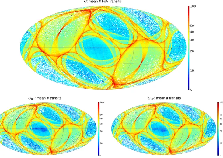
The results in DR2 are based on the first 22 months of Gaia data, taken between 25 July 2014 and 23 May 2016. For the variability analysis we made use of the photometric time se- ries in the G,GBP, andGRP bands, using field-of-view (FoV) averaged transit photometry. An exception to this was the anal- ysis of short-timescale variables, for which some per-CCDG- band photometry was also analysed, but not published. The pho- tometry is described in detail in Evans et al. (2018) and Riello et al. (2018). We emphasise that owing to the tight DR2 data- processing schedule, we only had access to a preliminary ver- sion of the DR2 astrometric solution (Lindegren et al. 2018), on which our results are based. No radial velocity data or astrophys- ical parameters were available during our processing.
2.1. Relative completeness
As a consequence of theGaiascanning law, the sky-coverage is rather non-uniform for the 22 months of DR2 data, resulting in sky-coverage gaps when selecting a certain minimum number of FoV transits. In our processing we used cuts of≥2,≥12, and
≥20G-band FoV transits, which we discuss in Sect. 3. Figure 1 shows the effect of these cuts on the sample of all available time series at the time of processing. Assuming that all sources with
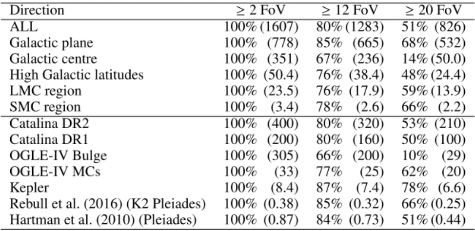
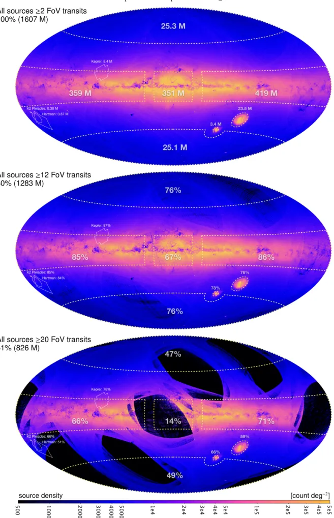
≥2 FoV transits are bona fide sources, these figures show that a cut of≥12 FoV transits results in a relative completeness of 80%, and a cut of≥ 20 FoV transits results in a relative com- pleteness of only 51%. It can generally be expected that these relative completenesses are an upper limit to the absolute (sky) completeness, which is assessed in detail in the follow-up vari- ability papers mentioned in the introduction. Arenou et al. (2018) conclude that the catalogue is mostly complete, in the absolute sense, roughly between magnitudes 7 and 17, and incomplete be- yond. For a first-order relative completeness assessment in cer- tain general Galactic directions, we introduce the following re- gions and compute theGaiasource count in each of them:
– Galactic plane30◦<l<330◦ & |b|<15◦
– Galactic centre20◦ >l>340◦ &|b|<15◦
– High Galactic latitudes|b| >45◦ , excluding a 10◦ radius around the SMC
– LMCregion within a radius of 7.5◦ from Galactic coordi- natesl=280.47◦,b=−32.89◦
– SMC region within a radius of 2.5◦ from Galactic coordi- natesl=302.81◦,b=−44.33◦
We repeat this for the (approximate) sky footprints of various external catalogues, list the results in Table 1 and display the regions in Fig. 1. It shows that a (maximum) completeness of between 70–85% for≥ 12G-band FoV transits and a relative completeness of between 50–70% for≥20G-band FoV transits can be expected. The bottom panel of Fig. 1 shows that various sky regions are not or only partially sampled for≥20 FoV: the Galactic centre region, for example, has a relative completeness of only 14%.
We remark that the numbers in Table 1 and Fig. 1 do not correspond exactly to the number of sources published in the gaia_sourcetable of DR2 because various source filters in the globalGaiaprocessing chain were applied before and after the variability processing. The derived percentages match very well, however, and they are relevant for the presented discussion.
2.2. Outliers and calibration errors
Various issues are visible in the current photometric data. Some of them are caused by instrumental effects, while others are sky related. Improved calibration strategies and careful flagging of these events are being designed and will be implemented in the chain of processing systems that convert the raw data into cali- brated epoch photometry for the nextGaiaData Release. Some of these issues are also described in Evans et al. (2018):
– hot pixel columns are not yet treated,
– poor background estimates exist for some observations, – observations close to bright sources can have biased back-
ground estimates or might even be spurious detections due to diffraction spikes,
– spatially close sources can have scan-angle direction depen- dent outliers,
– isolated sources can still be affected through overlap of the two FoVs.
It is expected that a certain fraction of observation affected by these issues has not been flagged and hence users should be aware of such unflagged outliers in the published data. We dis- cuss variability flagging in more detail in Sect. 4.1.
In addition to the flagging of observations, the Gaia data processing consortium has applied various filters that remove sources that are affected by specific calibration issues; see Gaia Collaboration et al. (2018a) for more details.
3. DR2 variability data processing and analysis The general variability data processing has been described in de- tail in our DR1 paper (Eyer et al. 2017), to which we refer here.
We here only summarise the main aspects that are specific to the DR2 release. More exhaustive information is provided in the DR2 documentation.
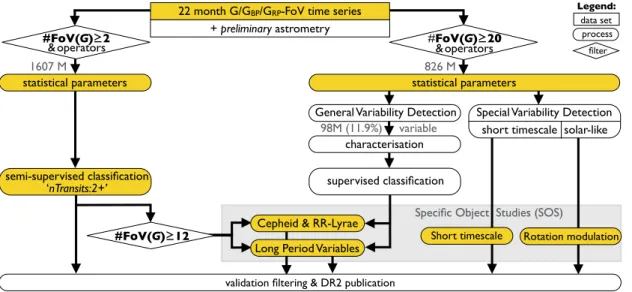
The variability processing is summarised in Fig. 2, and the number of sources involved at various levels of the processing is indicated in the diagram. The processing followed two main paths: one starting from 1607 million sources with≥2G-band FoV transits (hereafter geq2), and the other from 826 million
Table 1: Relative source counts for sources with ≥2 G-band FoV transits, illustrating the decrease in relative completeness for source sets with ≥12 and ≥20G-band FoV transits, as applied in our processing. The top part specifies the numbers for some generic directions in the Galaxy, as defined in Sect. 2.1 and illustrated in Fig. 1. The bottom part specifies the numbers for several external catalogues, listing the Gaiasource counts in their approximate sky footprints (not their source cross-match counts). In parenthesis, we provide the actualGaiasource counts in millions. Estimates of the absolute completeness of the published variable samples are presented in Tables 2 and 3.
Direction ≥2 FoV ≥12 FoV ≥20 FoV
ALL 100% (1607) 80% (1283) 51% (826)
Galactic plane 100% (778) 85% (665) 68% (532)
Galactic centre 100% (351) 67% (236) 14% (50.0)
High Galactic latitudes 100% (50.4) 76% (38.4) 48% (24.4)
LMC region 100% (23.5) 76% (17.9) 59% (13.9)
SMC region 100% (3.4) 78% (2.6) 66% (2.2)
Catalina DR2 100% (400) 80% (320) 53% (210)
Catalina DR1 100% (200) 80% (160) 50% (100)
OGLE-IV Bulge 100% (305) 66% (200) 10% (29)
OGLE-IV MCs 100% (33) 77% (25) 62% (20)
Kepler 100% (8.4) 87% (7.4) 78% (6.6)
Rebull et al. (2016) (K2 Pleiades) 100% (0.38) 85% (0.32) 66% (0.25) Hartman et al. (2010) (Pleiades) 100% (0.87) 84% (0.73) 51% (0.44)
sources with ≥20G-band FoV transits (hereafter geq20). The
≥ Xmeans aG-band time series withX non-null and positive FoV flux observations, but before the variability filters were ap- plied that are described in Sects. 4.1 and 4.2.
The first path resulted in the publishednTransits:2+classifi- cation results, as described in Sect. 4.3, as well as in a split-off path with≥12G-band FoV transits (hereafter geq12) that served as one of the inputs for the SOS modules: SOS Cep and RRL (Clementini et al. 2016, 2018) and SOS LPV (Mowlavi et al.
2018).
The second path leads to the majority of the pipelines and SOS results, as described in Sect. 4.4. It had two different vari- ability detection methods. The first is a ‘general’ variability de- tection, defined by a classifier trained on known cross-matched constant objects1 from OGLE4 (Soszy´nski et al. 2012), Hippar- cos (ESA 1997), the Sloan Digital Sky Survey (SDSS) (Ivezi´c et al. 2007), and classified constants, as well as many additional catalogues for variables (Rimoldini & et al. 2018). The second consists of multiple dedicated variability detection methods: one tuned to detect short-timescale variables and another to rota- tion modulation effects, which were subsequently followed by their associated SOS modules: SOS short timescale (Roelens et al. 2018) and rotation modulation (Lanzafame et al. 2018), analysing these sources in more detail. The general variabil- ity detection was followed by a generic multi-harmonic Fourier modelling based on the periodogram peak-frequency of an un- weighted least-squares period search. Various classification at- tributes were derived from this model and the time-series sta- tistical parameters, on which the classifier for the geq20 path was trained. The classified RR Lyrae stars, Cepheids, and LPVs were subsequently fed into the corresponding modules SOS Cep&RRL and SOS LPV, being their second input source. All modules of the variability pipeline include validation rules to en- sure that the output values are within acceptable ranges, which allowed us to identify issues early on in the processing.
An accounting of the number of sources published in the classification and SOS modules is given in Fig. 3. It shows that of the 550 737 unique variable sources, 363 969 (66%) appear
1 The least variable sources found inftp://ftp.astrouw.edu.pl/
ogle/ogle4/GSEP/maps/
in the classification results (Sect. 4.3) and 390 529 (71%) in SOS (Sect. 4.4). For several variability types, 203 681 sources (37%) appear in both, while the rest of the sources appear only in either classification (160 288, i.e. 29%) or SOS results (186 768, i.e. 34%). Note that the number appearing in both clas- sification and SOS tables (203 681) is 721 more than the sum of overlapping types shown in Fig. 3 because these are cases of dif- ferent assigned types in classification and SOS tables, which are omitted from the figure.
Depending on the type of object, there might only exist either a classification or SOS result. SOS results have generally lower contamination than the classification results and contain various type-specific astrophysical parameters that can be used to obtain more detailed information (such as the period), although this in- formation might be available for a less sky-uniform sample due to the minimum number ofG-band FoV observations of 12 or 20, depending on the SOS type. The classification contains only a la- bel and ‘score’ and has generally higher contamination rates, but it contains larger samples that are (more) uniformly distributed over the sky due to the minimum number ofG-band FoV obser- vations, which are 5 for RR Lyrae, 6 forδScuti and SX Phoeni- cis, 9 for Cepheids, and 12 for LPVs. These differences between classification and SOS in contamination rate and sample size are part of the pipeline design in which classification results feed into most of the SOS modules, as shown in Fig. 2 and discussed in more detail in the DR1 paper Eyer et al. (2017).
4. Results
4.1. Observation filtering and operators
The variability processing makes use of photometric data pro- vided in units of fluxes (e/s), and then converts them into magni- tudes using the magnitude zero-points defined in Evans et al.
(2018). In our pipeline, this transformation is done by our GaiaFluxToMagOperatoroperator. Several additional opera- tors were used to remove FoV transits by flagging and filtering them when they did not meet the required criteria, that is, when they were of insufficient quality. The chain of consecutive op- erators is described briefly here, for more details see the DR2 documentation:
– RemoveNaNNegativeAndZeroValuesOperator flagged and removed transits with NaN, negative, or zero flux values.
– RemoveDuplicateObservationsOperator flagged and re- moved pairs of transits with too close observation times (es- sentially one transit from the pair was incorrectly assigned to the source). This operator was responsible for the majority of the transit removals forGmagnitudes brighter than∼8, see Mowlavi et al. (2018) for more details.
– GaiaFluxToMagOperator converted the Gaia fluxes into magnitude using the Gaia zero-point magnitudes.
– ExtremeValueCleaningflagged and removed transits with unrealistically faint magnitudes. The cut values were chosen to beG≥25,GBP≥24, andGRP≥22.
– ExtremeErrorCleaningMagnitudeDependentflagged and removed transits with extreme magnitude errors. ForG, we used both a lower (0.01%) and upper (99.7%) threshold based on the observed distribution of transit magnitude er- rors (as a function of magnitude), while forGBPandGRP, we used only an upper threshold (99.9%).
– RemoveOutliersFaintAndBrightOperatorflagged and re- moved the time-series outliers of the source. Different crite- ria were used to account for the distribution of magnitudes or of the magnitude errors in the time series.
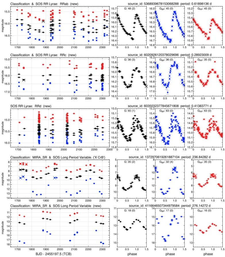
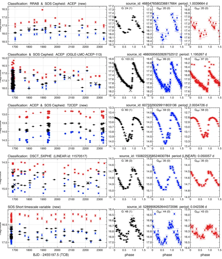
The time series following the above last operator was then the input for the different variability modules, and all transits that were flagged and filtered in the operator chain can be identified in the published time series by the rejected_by_variability flag (see Sect. 4.2). The re- sulting number of selected (i.e. not-rejected) transits can be found in the num_selected_g_fov/bp/rp fields of the vari_time_series_statisticstable. In Figs. 6, 7, and 8 the rejected transits are plotted as crosses. However, some SOS mod- ules (e.g. SOS Cep and RRL, SOS rotation modulation) applied individual stricter conditions that were tuned for their analysis.
We note that the SOS short timescale module also used another operator,RemoveOutlierPerTransitOperator, to remove CCD outliers per transit.
The sky distribution of the selected number of transits in the G,GBP, andGRPtime series are shown in Fig. 9 for all 550 737 published sources. The distribution of the mean values per sky- pixel is dominated by the scanning law, which is also visible in the large masked regions of the≥20 FoV panel of Fig. 1. Fig- ure 10 shows a histogram of the time-series lengths. The mini- mum number of transits inGis 5.
4.2. Time series, statistics, and variability flag
The full list of variable stars published in DR2 can be easily identified in the gaia_source table by the field phot_variable_flag, which is set to VARIABLE, while for all other sources it is set to NOT_AVAILABLE. The time series of all variable stars are published inG,GBP, andGRP. In con- trast to DR1, the time series are no longer provided in a separate archive table, but instead are accessible in a Virtual Observatory Table2(VOTable) linked3via the fieldepoch_photometry_url in the gaia_source table. For various reasons, a fraction of the transit observations was not photometrically processed in DR2, resulting in null values. The variability processing flags
2 Seehttp://www.ivoa.net/documents/VOTable/
3 For tutorials on using this datalink, see the Gaia archive help web-
pagehttp://gea.esac.esa.int/archive-help. Time-series bulk
download is possible fromhttp://cdn.gea.esac.esa.int/Gaia/.
per FoV transit (see previous section) are provided in the col- umnrejected_by_variability of the VOTable epoch pho- tometry. Additional flags from the photometric processing are available for transits in the columnrejected_by_photometry.
Unchanged from DR1 is the expression of observation time in units of barycentric JD (in TCB) in days−2 455 197.5, see DR2 documentation or Eyer et al. (2017) for more details.
All time series are provided in both flux and magnitude, where the flux is provided with the associated standard error.
The magnitude-transformed error value is omitted given its non- symmetric nature4. The Vega-system flux to magnitude zero- points are defined in Evans et al. (2018).
Several basic statistical parameters of the cleaned5 time series are listed in the vari_time_series_statistics ta- ble. The variable stars will furthermore have an entry in at least one of the vari_* tables, see Fig. 3 for their numbers.
An overview of time-series statistics perGaia band and types is provided in Tables 4 and 5. The mean magnitudes pro- vided ingaia_source(phot_g/bp/rp_mean_mag) differ from the mean magnitudes in vari_time_series_statistics (mean_mag_g_fov/bp/rp) because they are calculated dif- ferently (see Evans et al. 2018) and because the filter- ing of the light curves was different; furthermore, the gaia_source mean photometry can be absent, but present in thevari_time_series_statisticstable (together with the related time series in epoch_photometry_url) because vari- ous filters were applied by the photometry pipeline. The sky and median magnitude distributions of these sources are shown in more detail in Figs. 4 and 5.
4.3. Classification
In DR2 we introduce the output of the semi-supervised classi- fier targeted to identify high-amplitude variable stars over the whole sky, resulting from the geq2 path described in Sect. 3.
This is the aim of thenTransits:2+classification. Owing to the limited 22 months of data and rejected observations, the num- ber of FoV transits per source can be very small, prohibiting the use of Fourier modelling parameters for a large portion of the sources. Previous studies such as Ivezi´c et al. (2000) and Her- nitschek et al. (2016) have shown that it is still possible to iden- tify good RR Lyrae star candidates with just a few observations.
Our classifier was trained to identify high-amplitude variables of the type of RR Lyrae stars (anomalous RRd, see Soszy´nski et al.
2016 ; RRd, RRab, RRc), LPV (Mira-type and semi-regulars), Cepheids (anomalous Cepheids,δCepheids, type-II Cepheids), δ Scuti and SX Phoenicis stars, amongst the many other (non-)variable source types that exist. These classes can be found in the Gaia archive vari_classifier_result table with best_class_name = ARRD, RRD, RRAB, RRC, MIRA_SR, ACEP, CEP, T2CEP,and DSCT_SXPHE, respectively. Each en- try has an associatedbest_class_scorebetween 0 and 1. Ad- ditional (non-published) classes were included in the predic- tion types, see Rimoldini & et al. (2018) for all details. De- scriptions of the classifier and the published classes can be found in theGaiaarchivevari_classifier_definitionand vari_classifier_class_definitiontable, respectively.
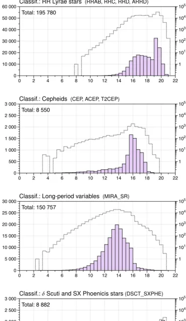
The sky and magnitude distribution of the published classes, grouped by main type, is shown in the left panels of Figs. 4 and 5, and some time-series examples are shown in Figs. 6 and 7.
4 Practical approximation:magerroru(2.5/ln(10))·f luxerror/f luxvalue
5 Selecting FoV transits withrejected_by_variability=false
The published source samples were cleaned to reduce con- tamination levels caused by data and processing artefacts, as well as by genuine variability of other types. The results and details of this procedure are fully detailed in Rimoldini & et al. (2018).
The output of this classifier for sources containing at least 12 measurements in theirG-band time series was used as one of the two inputs to the SOS of RR Lyrae stars, Cepheids, and LPV, as shown in Fig. 2, hence accounting for the overlap between classification and SOS results in Fig. 3. Some SOS modules may reclassify the type in the SOS tables, see Sect. 4.6 An overview of the inferred completeness and contamination with respect to several cross-match catalogues of the different types is provided in Table 2.
4.4. Specific Object Studies
In the geq20 path described in Sect. 3, potential variable type candidates that are identified in the supervised classification and special variability detection (SVD) parts of the pipeline were analysed in SOS modules, which often derived a model and/or additional astrophysical properties. The SOS modules can also decide whether an object is not of the expected type and as a re- sult not produce any output for it. We recall that a sub-sample of the sources processed in the geq2 path was processed by some SOS modules (see Fig. 2). We present short descriptions of the SOS modules used for DR2 below .
The sky and magnitude distribution of each published type is shown in the right panels of Figs. 4 and 5, and example light curves are presented in Figs. 6, 7, and 8. Because SOS mod- ules can be fed by (partially) independent pipeline-paths, it is not excluded that a source is listed in multiple SOS tables, as discussed in Sect. 4.5, or has a different classification and SOS type, as discussed in Sect. 4.6. Despite extensive validation ef- forts, the nature of our processing is an automated and statistical characterisation of the sources, hence identified sources that are not yet known in the literature should be considered to be can- didates, unless they are specifically validated in one of the SOS articles referenced below.
An overview of the inferred (absolute) sky completeness and contamination with respect to existing catalogues of the differ- ent types is provided in Table 3; see sections below and the ref- erences therein for more details. Many of the listed reference catalogues have a (very) limited sky coverage, and hence the contamination might be locally biased. To assess contamination in the whole SOS published samples, we performed the follow- ing additional visual inspection for each SOS output separately:
we took a random sample of 500 sources from the published results, as well as a sky-uniform6 sample of 500 sources (non- overlapping with the random sample). The former sample fol- lows the general sky distribution as shown in Fig. 4, while the latter achieves an almost sky-uniform sampling and hence also draws samples from very low density regions. The results are summarised below for each SOS result:
– Cepheids: 5% of the random sample was visually rejected, of which 3% might be due to binaries or ellipsoidals. Most of this sample is located in the Magellanic Clouds.
Of the sky-uniform sample, 15% was visually rejected, of which 11% might be due to binaries or ellipsoidals.
6 Approximate sky-uniform sampling is achieved by first grouping the
sources in 12 288 bins (level 5 HEALPix, see Górski et al. 2005) of
about 3.6 deg2and then randomly drawing non-empty pixels and ex-
tracting a source at random from it.
– RR Lyrae stars: 9% of the random sample was visually re- jected, of which 4% are faint (20.0<G<20.7 mag).
Of the sky-uniform sample, 12% was visually rejected, of which 5% are faint (19.9<G<20.7 mag).
– Long-period variables: 0.1% (1) was visually rejected; it looks like a young stellar object, confirmed by its position in the Hertzsprung-Russel (HR) diagram.
– Short-timescale variability: 0.3% was visually rejected, and about 24% seem to exhibit short-timescale periodic vari- ability, but this can currently not be confirmed with a high confidence.
– Rotation modulation: 0.3% was visually rejected.
These identified contamination rates are compatible7 with the cross-match sample contamination rates found in Table 3.
4.4.1. Cepheids and RR Lyrae stars
The SOS Cepheids and RR Lyrae module (SOS Cep and RRL, Clementini et al. 2016, 2018), confirmed, characterised, and sub- classified in type 140 784 RR Lyrae stars and 9 575 Cepheids of the candidates provided by the classifiers. The module can re- classify the type provided by the classifiers from Cepheid to RR Lyrae star, and vice versa. Amongst the RR Lyrae stars, the fol- lowing number of sub-types were identified: 98 026 fundamental mode pulsators (RRab), 40 380 first-overtone pulsators (RRc), and 2378 double-mode pulsators (RRd). Amongst the Cepheids, there were 8890δCepheids, 100 anomalous Cepheids, and 585 type II Cepheids, of which 223 were classified as BL Her, 253 as W Vir, and 109 as RV Tau.
A rough estimate of completeness and contamination was obtained by comparing our samples with OGLE catalogues of RR Lyrae stars and Cepheids in the Large Magellanic Cloud (LMC). We selected an area of the LMC centred atα=83◦and δ=−67.5◦ and extending from 67.5◦ to 97.5◦in right ascension and from−63.5◦to−73◦in declination. Completeness of our RR Lyrae sample in this area is 64%, and contamination is less than 0.1%. In the same area, the Cepheid sample is 74% complete with 100% purity. A more in-depth description and analyses of the results, as well as the origin of the Bulge completeness rates quoted in Table 3, can be found in Clementini et al. 2018. Of the 599 Cepheids and 2595 RR Lyrae stars that were identified in DR1 (Clementini et al. 2016; Eyer et al. 2017), 533 Cepheids and 2517 RR Lyrae stars are also available in this DR2 release.
4.4.2. Long-period variables
Long-period variables are red giants that are characterised by long periods and variability amplitudes of up to a few mag- nitudes. They are identified by classification as MIRA_SR. On the basis of data available for DR2, CU7 selected 151 761 LPV candidates that fulfil the selection criteria for LPVs, which in- cluded a minimum of 12 points inG, aGBP−GRPcolour higher than 0.5 mag, a variability amplitude (quantified with the 5%- 95% trimmed range inG) larger than 0.2 mag, and a correlation betweenGandGBP−GRP higher than 0.5. Of these, 150 757 are published in the classification table, and 89 617 have SOS results. The detailed distribution into these two tables is indi- cated in Fig. 3. The SOS LPV module processes LPV candi- dates when their period is longer than 60 days. The steps applied
7 For Cepheids and RR Lyrae stars, the contamination rates quoted in
Table 3 were taken from these analyses because contaminants from the OGLE-IV catalogues were already removed from the published results;
see Clementini et al. (2018) for more details.
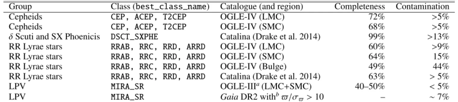
Table 2: Classification (absolute) completeness and contamination estimates with respect to available cross-matched reference cat- alogues. For more details on the validation of the classification results, we refer to Rimoldini & et al. (2018).
Group Class (best_class_name) Catalogue (and region) Completeness Contamination
Cepheids CEP, ACEP, T2CEP OGLE-IV (LMC) 72% >5%
Cepheids CEP, ACEP, T2CEP OGLE-IV (SMC) 68% >5%
δScuti and SX Phoenicis DSCT_SXPHE Catalina (Drake et al. 2014) 99% >13%
RR Lyrae stars RRAB, RRC, RRD, ARRD OGLE-IV (LMC) 60% >9%
RR Lyrae stars RRAB, RRC, RRD, ARRD OGLE-IV (SMC) 64% 15%
RR Lyrae stars RRAB, RRC, RRD, ARRD OGLE-IV (Bulge) 49% 44%
RR Lyrae stars RRAB, RRC, RRD, ARRD Catalina (Drake et al. 2014) 63% >5%
LPV MIRA_SR OGLE-IIIa(LMC+SMC) 40–50% <5%
LPV MIRA_SR GaiaDR2 withb$/σ$>10 – ∼7%
Notes.(a)Estimates are restricted to sources with peak-to-peak amplitude>0.2 mag.(b)$andσ$refer to the DR2 parallax and associated error.
Table 3: SOS (absolute) completeness and contamination estimates with respect to cross-matched reference catalogues. Processing paths are based on the number of selected FoV transits, as shown in Fig. 2 and discussed in Sect. 3. See Sect. 4.4 for additional contamination rate estimates for random and sky-uniform samples. For more details on the validation of the SOS type results, see Sect. 4.4 and the references therein.
Processing path SOS Type Catalogue (and region) Completeness Contamination
geq12 & geq20 Cepheids OGLE-IV (LMC, limited region) 74% ∼5%a
geq12 & geq20 Cepheids OGLE-IV (Bulge) 3% b
geq12 & geq20 RR Lyrae stars OGLE-IV (LMC, limited region) 64% ∼9%a
geq12 & geq20 RR Lyrae stars OGLE-IV (Bulge) 15% b
geq12 & geq20 LPV OGLE-IIIc(SMC+LMC) ∼30% <few%
geq12 & geq20 LPV OGLE-IIIc(SMC+LMC) ∼30% <few%
geq20 Short timescale OGLE-II, III, IV (MCs) 0.05% 10–20%
geq20 Rotational modulation The Pleiades (Hartman et al. 2010) 0.7 – 5.0% <50%d
Notes. (a) Estimated from non-cross-match random samples inspection discussed in Sect. 4.4, extending partially beyond OGLE-IV footprint.
(b)No reliable contamination rate for the Bulge has been derived, but in the Galactic disk footprint (see Udalski 2017), contamination of the SOS
Cepheids and RR Lyrae stars might be of the order of several tens of percent (A. Udalski, priv. comm. based on unpublished OGLE-IV data).
(c) Estimates are restricted to sources with a peak-to-peak amplitude>0.2 mag and periods longer than 60 days.(d) The 50% ‘contamination’
quantifies the non-occurrence in the reference catalogue; the actual contamination of grazing binaries is estimated to be<1%, see Sect. 4.4.4.
include period search, the determination of bolometric correc- tion fromGBP andGRP fluxes, the identification of red super- giants, and the computation of absolute magnitude. It must be noted that all LPV specific attributes published in DR2 that de- pend on the parallax must be recomputed based on the published parallaxes, because these LPV-specific attributes were computed based on an older version of the parallaxes that was available at the time of variability processing within the consortium. We re- fer to Mowlavi et al. (2018) for additional information. The light curves of all LPV candidates, whether identified in the classifi- cation table or in the SOS table, are published in DR2.
The completeness and contamination numbers for the LPV candidates towards the Magellanic Clouds are computed relative to a sub-sample of the OGLE-III catalogue of LPVs (Soszy´nski et al. 2009, 2011). The sub-sample consists of all OGLE-III LPVs withI-band amplitude larger than 0.2 mag for the classifi- cation completeness and contamination estimates, and is further restricted to the OGLE-III LPVs with periods longer than 60 d for the SOS completeness and contamination estimates. Addi- tionally, an all-sky contamination estimate is provided forGaia LPV candidates that have small relative parallax uncertainties based on their position in the HR diagram. The main contami- nants in this sample consist of young stellar objects. Details of SOS LPV processing and estimates of completeness and con- tamination can be found in Mowlavi et al. (2018), where the DR2 data set of LPV candidates are presented and further analysed.
4.4.3. Short-timescale variability
Short-timescale variable sources are astrophysical objects show- ing any variability in their optical light-curve with a character- istic timescale of the variation shorter than 1 d (Roelens et al.
2017). A variety of astronomical objects are known to exhibit such fast photometric variations, including both periodic and transient variability, involving amplitudes from a few millimag- nitudes to a few magnitudes, with different variability character- istics and phenomena at the origin of variation, from pulsations to flares to eclipsing systems. The diverse variability types tar- geted by the short-timescale module range from short-period bi- nary stars to pulsating white dwarfs (e.g. ZZ Ceti stars or V777 Herculis stars) and cataclysmic variables such as AM CVn stars.
However, for theGaiaDR 2, the short-timescale variability pro- cessing is oriented towards periodic variability, and the exact variable type of the detected short-timescale candidates is not yet determined. Both the investigation of transient variability (Wev- ers et al. 2018) and the further classification of the candidates are foreseen for the futureGaiadata releases.
As mentioned previously, the identification of the short- timescale variable candidates published inGaiaDR2 involves particular variability detection methods that are specifically tuned to detect fast photometric variability, complementarily to the general variability detection approach (which may miss some of these events because they are so fast). These methods are ap- plied to a preselected subset of the Gaia data set (Eyer et al.
2017): forGaiaDR 2, the short-timescale variability analysis is restricted to relatively faint sources (G∼16.5−20 mag) whoseG per-CCD time series indicates that they are likely to show rapid variations (Roelens et al. 2018). Consequently, the candidates resulting from the short-timescale module are expected to over- lap with other short-period SOS variables such as RR Lyrae and δScuti stars with periods shorter than 1 d, even though not there is no complete overlap with these SOS variable candidates.
The SOS short-timescale module identified 3018 short- timescale, suspected periodic candidates. These bona fide, short- timescale, suspected periodic candidates were identified based on the combination of the variogram analysis (Eyer & Gen- ton 1999; Roelens et al. 2017), least-squares frequency search (Zechmeister & Kürster 2009), analysis of the environment of candidate sources over the sky, and a series of selection criteria from various statistics, such as the Abbe or inter-quartile range (IQR) values in the three bands (G,GBPandGRP).
Completeness and contamination numbers for the short- timescale variable candidate sample, estimated by comparing OGLE-II, III, IV, and Gaiadata in the Magellanic Clouds, are listed in Table 3. Furthermore, about 50% of the known OGLE- III and IV variables belonging to the short-timescale sample in these regions are longer period variables (i.e. with period>1d).
However, most of these contaminant sources have periods of a few days and quite high amplitudes, hence although they are no true short-period variables, their presence in the short-timescale published sample is justified. A more detailed description and analysis of the results can be found in Roelens et al. (2018).
4.4.4. Rotational modulation
Stellar flux modulation induced by surface inhomogeneities and rotation is searched for in a region of the HR diagram, broadly embracing stars of spectral type later than F on the main se- quence. This type of variability, often indicated in the literature as BY Draconis stars (BY Dra) regardless of possible binarity, is an indication of active regions (dark spots and bright facu- lae on the stellar photosphere) that are produced by stellar mag- netic activity. The evolution of stellar magnetic fields, similar to solar fields, produces variability phenomena on a wide range of timescales (see e.g. Lanza et al. 2004; Distefano et al. 2012;
Lanza et al. 2006, and references therein); one of the most promi- nent phenomena is the rotational modulation itself, from which the stellar rotation period can be inferred.
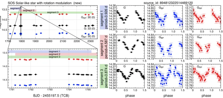
The variability pipeline comprises two packages dedicated to the detection and characterisation of solar-like stars with ro- tational modulation. First, solar-like variable candidates are se- lected, and if they are confirmed, they are studied in more detail to determine stellar rotation periods and other properties. Fig. 8 shows one of the published light-curves together with the seg- ments in which a significant (similar) period was detected.
We detected some 7×10⁵ periodic variables in the pre- selected HR diagram region, which excludes areas populated by pulsating variables. The remaining expected main contaminants are eclipsing binaries and spurious detections derived from an incomplete sampling. To filter out these cases as well as possi- ble, we applied filters that exclude sources whose period-folded light curves have a significantly uneven distribution in phase, with significant gaps, and are far from being sinusoidal (see Lan- zafame et al. 2018, for details). The final DR2 clean sample con- tains 147 535 rotational modulation candidates and fills 38% of the whole sky when divided into bins of ≈0.84 deg2 (level 6 HEALPix), see for example Fig. 4.
An estimate of the final completeness and contamination of the DR2 rotational modulation variables is hampered by the fact that the occurrence rate of the BY Dra phenomenon is largely unknown so far. It is expected that all low-mass dwarfs are magnetically active to some extent, and the rotational modula- tion detectability essentially depends on the instrumental sensi- tivity, and also on the active region distribution and the phase of the magnetic cycle at the epoch of observations. New low- mass dwarfs displaying rotational modulation are continuously detected with the ever-wider span and increasing sensitivity of modern surveys, none of which has the full sky coverage ca- pabilities ofGaia, however. At this stage, it is possible to per- form some meaningful comparison only with the Hartman et al.
(2010) and Rebull et al. (2016) observations of the Pleiades, with which, nevertheless, the DR2 geq20 sky coverage still overlaps only marginally. Assuming that the Hartman et al. (2010) cat- alogue lists all the BY Dra in its FoV down toG ≈ 14.5, we estimate that the completeness of the BY Dra sample is 14%
down toG ≈ 16.5 in the overlapping field. Assuming that this value is uniform over the whole sky, we estimate a completeness upper limit of 5%. At the other extreme, we may assume that all low-mass dwarfs are BY Dra variables. Then, comparing with all stars observed byGaiain the same sky region and magnitude range, we estimate a lower completeness limit of 0.7%.
We may roughly estimate an upper limit for contamination by assuming that theGaiaBY Dra detections that are not present in the Hartman et al. (2010) or in the Rebull et al. (2016) sample in the common region on the sky are variables of other types.
This upper limit is obviously largely overestimated given that no BY Dra catalogue can be deemed complete to date, as also testified by the fact that there are sources in the Hartman et al.
(2010) sample that are not contained in the Rebull et al. (2016) sample, and vice versa.
At the other extreme, we can make an educated guess re- garding the contamination of close grazing binaries that would be incorrectly classified as BY Dra because of the similarity of the light curves. If the orbital period is long, then the grazing eclipse occurs only in a small part of the orbit, and it does not look like rotation modulation. We assume an upper limit period of 10 days for this contaminating effect. The fraction of stars with such short-period companions is only about 2–5% (Ragha- van et al. 2010), of which only 2–5% are grazing binaries (at most), which means 0.04–0.25 % of the stars, while we did not yet take into account that for most binaries, the secondaries are substantially smaller. Even though we cannot consider the rota- tion modulation sample a random subset of G and later-type stars (which is the assumption in above estimate), it seems unlikely that this type of contamination would exceed 1%. The same con- clusion is reached from our internal validation against known and newly identified (but not published) eclipsing binaries, based on which, we estimate an upper limit of 0.5% grazing contam- ination. From the estimated grazing binary contamination and non-occurrence in the reference catalogue discussed above, we estimate a contamination level ranging from<1% to≈50%, as listed in Table 3. More details on the SVD solar-like and SOS rotational modulation packages and results can be found in Lan- zafame et al. (2018).
4.5. Sources with multiple SOS types
There are 80 sources in DR2 with an entry in more than one SOS table. These cases are all overlaps between short-timescale objects and RR Lyrae stars (72), Cepheids (5), and rotation mod-
ulation objects (3), all of which are justified by their overlapping type definition. No overlap is found with long-period variables.
4.6. Sources with different classification and SOS type Differences are found between classification types (as obtained by supervised classification in the geq2 path) and the types that are eventually derived in SOS results (either from the geq12 or geq20 paths). In particular, one source was classified as DSCT_SXPHE, but also appears in SOS rotational modulation.
Similarly, one source was classified as MIRA_SR, was not con- firmed by SOS LPV, but appears in SOS rotational modulation.
Of the sources classified as a Cepheid (any type), 6 appear in more than one SOS table. One is a confirmed SOS Cep and also appears in SOS short timescale, while 3 appear as SOS rotational modulation and 2 as SOS short timescale. Of the sources classi- fied as an RR Lyrae star (any type), 70 appear in the SOS short timescale table, one was instead confirmed as a Cepheid by SOS (shown in the top panel of Fig. 7), and many were confirmed as RR Lyrae star by SOS. Overall, a reassignment of the type from RRL into Cep by SOS occurred in 618 cases, but only in 77 cases from Cepheid to RR Lyrae star by SOS. We have decided to retain the original classification type despite the possible reas- signment by the SOS Cep&RRL module or in cases where they were confirmed as another type by SOS modules.
5. Conclusions
In this secondGaiadata release, a sample of 550 737 variable sources with their three-band time series and analysis results has been released to the astronomical community, showcasing samples of high-amplitude variable candidates distributed over (a large portion of) the whole sky. It demonstrates the immense potential ofGaiadata to provide an unbiased all-sky photomet- ric survey together with astrometric and spectroscopic data. Al- though the variability analyses in DR2 did only mildly rely on the astrometric data and on none of the spectroscopic data, this dependence will become much heavier in future data releases.
Several caveats have been outlined in this paper:
– Most provided stellar samples are rather incomplete as a re- sult of the current state of data calibration (e.g. even well- known variables might be missing) or the limited scanning law coverage for the minimum number of selected observa- tions,
– known incomplete flagging of outliers in the time series, – existence of uncalibrated systematics or spurious calibration
error signals in some of the time series,
– the probabilistic and automated nature of this work im- plies certain completeness and contamination rates (Tables 2 and 3), hence even well-known literature sources could be misidentified.
Overall, we estimate8 to have identified the following num- bers of new variables: a few hundred Cepheids, a few tens of thousand RR Lyrae stars, about one hundred thousand stars with rotation modulation, several tens of thousand long-period vari- ables, a few thousandδScuti and SX Phoenicis stars, and a few thousand short-timescale variables. In total, this is about half of the variable sources released in this DR2. Compared to the DR1 example, we increased the sample size about 100 times, which is
8 From occurrence in a great variety of cross-match catalogues (most
of which are documented in the DR2 documentation), and taking into account that our results have a varying degree of contamination.
expected to result in a large number of novel studies, regardless of whether they are combined with existing data sets.
The next variability release will be based on data that are better calibrated yet again and on a longer time baseline. It will also include BP/RP spectrophotometry and radial velocities from RVS, which will allow us to improve the quality and quantity of theGaiaDR3 release.
Acknowledgements.
We dedicate this paper to our dear friend and colleague Jan Cuypers (1956-2017), whose passing has left a great void in our variability group. Thank you, Jan, for your friendship and lifelong contribution to science.
We would like to thank the referee, Andrzej Udalski, for various suggestions and providing so far unpublished OGLE-IV estimates that improved the contents of this paper. We thank Xavier Luri, Antonella Vallenari, and Annie Robin for valu- able feedback during the preparation of this paper. We also acknowledge Mark Taylor for creating and implementing new requested features in the astronomy- oriented data handling and visualization software TOPCAT (Taylor 2005). This work has made use of data from the ESA space missionGaia, processed by the GaiaData Processing and Analysis Consortium (DPAC).
Funding for the DPAC has been provided by national institutions, some of which participate in theGaiaMultilateral Agreement, which include, for Switzerland, the Swiss State Secretariat for Education, Research and Innovation through the ESA PRODEX program, the “Mesures d’accompagnement”, the “Activités Na- tionales Complémentaires”, the Swiss National Science Foundation, and the Early Postdoc. Mobility fellowship; Belgium, the BELgian federal Science Pol- icy Office (BELSPO) through PRODEX grants; for Italy, Istituto Nazionale di Astrofisica (INAF) and the Agenzia Spaziale Italiana (ASI) through grants I/037/08/0, I/058/10/0, 2014-025-R.0, and 2014-025-R.1.2015 to INAF (PI M.G.
Lattanzi); for France, the Centre National d’Etudes Spatiales (CNES). This re- search has received additional funding from: the Israeli Centers for Research Excellence (I-CORE, grant No. 1829/12); the Hungarian Academy of Sci- ences through the Lendület Programme LP2014-17 and the János Bolyai Re- search Scholarship (L. Molnár and E. Plachy); the Hungarian National Re- search, Development, and Innovation Office through grants OTKA/NKFIH K- 113117, K-115709, PD-116175, and PD-121203; the ÚNKP-17-3 program of the Ministry of Human Capacities of Hungary (Á.L.J.); the ESA Contract No. 4000121377/17/NL/CBi; and the Polish National Science Center through ETIUDA grant 2016/20/T/ST9/00170; Charles University in Prague through PRIMUS/SCI/17 award; and from the EuropeanResearch Council (ERC) under the European Union’s Horizon 2020 research and innovation programme (grant agreement N◦670519: MAMSIE).
References
Arenou, F., Luri, X., Babusiaux, C., et al. 2018, ArXiv e-prints [arXiv:1804.09375]
Clementini, G., Ripepi, V., Leccia, S., et al. 2016, A&A, 595, A133
Clementini, G., Ripepi, V., Molinaro, R., et al. 2018, ArXiv e-prints [arXiv:1805.02079]
Distefano, E., Lanzafame, A. C., Lanza, A. F., et al. 2012, MNRAS, 421, 2774 Drake, A. J., Graham, M. J., Djorgovski, S. G., et al. 2014, ApJS, 213, 9 ESA, ed. 1997, ESA Special Publication, Vol. 1200, The Hipparcos and Ty-
cho catalogues. Astrometric and photometric star catalogues derived from the ESA Hipparcos Space Astrometry Mission
Evans, D. W., Riello, M., De Angeli, F., et al. 2018, ArXiv e-prints [arXiv:1804.09368]
Eyer, L. & Genton, M. G. 1999, A&AS, 136, 421
Eyer, L., Mowlavi, N., Evans, D. W., et al. 2017, ArXiv e-prints [arXiv:1702.03295]
Gaia Collaboration, Brown, A. G. A., Vallenari, A., et al. 2018a, ArXiv e-prints [arXiv:1804.09365]
Gaia Collaboration, Brown, A. G. A., Vallenari, A., et al. 2016, A&A, 595, A2 Gaia Collaboration, Eyer, L., Rimoldini, L., et al. 2018b, ArXiv e-prints
[arXiv:1804.09382]
Górski, K. M., Hivon, E., Banday, A. J., et al. 2005, ApJ, 622, 759
Hartman, J. D., Bakos, G. Á., Kovács, G., & Noyes, R. W. 2010, MNRAS, 408, 475
Hernitschek, N., Schlafly, E. F., Sesar, B., et al. 2016, ApJ, 817, 73 Ivezi´c, Ž., Goldston, J., Finlator, K., et al. 2000, AJ, 120, 963 Ivezi´c, Ž., Smith, J. A., Miknaitis, G., et al. 2007, AJ, 134, 973
Lanza, A. F., Messina, S., Pagano, I., & Rodonò, M. 2006, Astronomische Nachrichten, 327, 21
Lanza, A. F., Rodonò, M., & Pagano, I. 2004, A&A, 425, 707
Lanzafame, A. C., Distefano, E., Messina, S., et al. 2018, ArXiv e-prints [arXiv:1805.00421]
Lindegren, L., Hernandez, J., Bombrun, A., et al. 2018, ArXiv e-prints [arXiv:1804.09366]
Molnár, L., Plachy, E., Juhász, Á. L., & Rimoldini, L. 2018, ArXiv e-prints [arXiv:1805.11395]
Mowlavi, N., Lecoeur-Taïbi, I., Lebzelter, T., et al. 2018, ArXiv e-prints [arXiv:1805.02035]
Palaversa, L., Ivezi´c, Ž., Eyer, L., et al. 2013, AJ, 146, 101
Raghavan, D., McAlister, H. A., Henry, T. J., et al. 2010, ApJS, 190, 1 Rebull, L. M., Stauffer, J. R., Bouvier, J., et al. 2016, AJ, 152, 113
Riello, M., De Angeli, F., Evans, D. W., et al. 2018, ArXiv e-prints [arXiv:1804.09367]
Rimoldini, L. & et al. 2018, A&A, in prep.
Roelens, M., Eyer, L., Mowlavi, N., et al. 2017, MNRAS, 472, 3230
Roelens, M., Eyer, L., Mowlavi, N., et al. 2018, ArXiv e-prints [arXiv:1805.00747]
Soszy´nski, I., Smolec, R., Dziembowski, W. A., et al. 2016, MNRAS, 463, 1332 Soszy´nski, I., Udalski, A., Poleski, R., et al. 2012, Acta Astron., 62, 219 Soszy´nski, I., Udalski, A., Szyma´nski, M. K., et al. 2009, Acta Astron., 59, 239 Soszy´nski, I., Udalski, A., Szyma´nski, M. K., et al. 2011, Acta Astron., 61, 217 Taylor, M. B. 2005, in Astronomical Society of the Pacific Conference Se-
ries, Vol. 347, Astronomical Data Analysis Software and Systems XIV, ed.
P. Shopbell, M. Britton, & R. Ebert, 29
Udalski, A. 2017, in European Physical Journal Web of Conferences, Vol. 152, European Physical Journal Web of Conferences, 01002
Wevers, T., Jonker, P. G., Hodgkin, S. T., et al. 2018, Monthly Notices of the Royal Astronomical Society, 473, 3854
Zechmeister, M. & Kürster, M. 2009, A&A, 496, 577
1 Department of Astronomy, University of Geneva, Ch. des Maillettes
51, CH-1290 Versoix, Switzerland
2 Department of Astronomy, University of Geneva, Ch. d’Ecogia 16,
CH-1290 Versoix, Switzerland
3 SixSq, Rue du Bois-du-Lan 8, CH-1217 Geneva, Switzerland
4 GÉPI, Observatoire de Paris, Université PSL, CNRS, Place Jules
Janssen 5, F-92195 Meudon, France
5 INAF Osservatorio di Astrofisica e Scienza dello Spazio di Bologna,
Via Gobetti 93/3, I - 40129 Bologna, Italy
6 Instituut voor Sterrenkunde, KU Leuven, Celestijnenlaan 200D,
3001 Leuven, Belgium
7 Institute of Astronomy, University of Cambridge, Madingley Road,
Cambridge CB3 0HA, UK
8 Large Synoptic Survey Telescope, 950 N. Cherry Avenue, Tucson,
AZ 85719, USA
9 Università di Catania, Dipartimento di Fisica e Astronomia, Sezione
Astrofisica, Via S. Sofia 78, I-95123 Catania, Italy
10 INAF-Osservatorio Astrofisico di Catania, Via S. Sofia 78, I-95123
Catania, Italy
11 University of Vienna, Department of Astrophysics, Tuerkenschanz-
strasse 17, A1180 Vienna, Austria
12 Department of Geosciences, Tel Aviv University, Tel Aviv 6997801,
Israel
13 Dipartimento di Fisica e Astronomia, Università di Bologna, Via
Piero Gobetti 93/2, 40129 Bologna, Italy
14 Departamento de Astrofísica, Centro de Astrobiología (INTA-
CSIC), PO Box 78, E-28691 Villanueva de la Cañada, Spain
15 School of Physics and Astronomy, Tel Aviv University, Tel Aviv
6997801, Israel
16 INAF-Osservatorio Astronomico di Capodimonte, Via Moiariello
16, 80131, Napoli, Italy
17 Dpto. Inteligencia Artificial, UNED, c/Juan del Rosal 16, 28040
Madrid, Spain
18 Department of Astrophysics/IMAPP, Radboud University, P.O.Box
9010, 6500 GL Nijmegen, The Netherlands
19 European Southern Observatory, Karl-Schwarzschild-Str. 2, D-
85748 Garching b. München, Germany
20 Laboratoire d’astrophysique de Bordeaux, Univ. Bordeaux, CNRS,
B18N, allée Geoffroy Saint-Hilaire, 33615 Pessac, France
21 Harvard-Smithsonian Center for Astrophysics, 60 Garden Street,
Cambridge, MA 02138, USA
22 Royal Observatory of Belgium, Ringlaan 3, B-1180 Brussels, Bel-
gium
23 Konkoly Observatory, Research Centre for Astronomy and Earth
Sciences, Hungarian Academy of Sciences, H-1121 Budapest, Konkoly Thege Miklós út 15-17, Hungary
24 Department of Astronomy, Eötvös Loránd University, Pázmány
Péter sétány 1/a, H-1117, Budapest, Hungary
25 Villanova University, Department of Astrophysics and Planetary
Science, 800 Lancaster Ave, Villanova PA 19085, USA
26 Faculty of Mathematics and Physics, University of Ljubljana, Jad-
ranska ulica 19, 1000 Ljubljana, Slovenia
27 Academy of Sciences of the Czech Republic, Fricova 298, 25165
Ondrejov, Czech Republic
28 Baja Observatory of University of Szeged, Szegedi út III/70, H-6500
Baja, Hungary
29 Université Côte d’Azur, Observatoire de la Côte d’Azur, CNRS,
Laboratoire Lagrange, Bd de l’Observatoire, CS 34229, 06304 Nice cedex 4, France
30 CENTRA FCUL, Campo Grande, Edif. C8, 1749-016 Lisboa, Por-
tugal
31 EPFL SB MATHAA STAP, MA B1 473 (Bâtiment MA), Station 8,
CH-1015 Lausanne, Switzerland
32 Warsaw University Observatory, Al. Ujazdowskie 4, 00-478
Warszawa, Poland
33 Institute of Theoretical Physics, Faculty of Mathematics and
Physics, Charles University in Prague, Czech Republic
34 Max Planck Institute for Astronomy, Königstuhl 17, 69117 Heidel-
berg, Germany
Table4:StatisticalparametersforthenTransits:2+classificationtypespublishedinDR2.The1%,50%(median),and99%percentileareprovidedforeachtype. GbandCepheidsaRRLyraestarsbLong-periodvar.cδSctandSXPhed FilterednumberofFoVtransits13271207196912246592164 Timeduration(d)513.15627.70667.73383.37588.36652.89426.47591.70638.78402.04572.46654.34 Meanobservationtime(d)1741.282018.522112.721800.952026.532156.081895.782037.132155.471862.232023.302142.49 Min.magnitude7.4815.6117.6013.3517.7519.818.0113.2517.0711.0619.5020.59 Max.magnitude8.0316.1518.2114.1018.4220.738.8414.0117.7911.3619.8021.09 Meanmagnitude7.8015.9117.9713.8118.1520.348.4713.6317.3511.2519.6920.84 Medianmagnitude7.7715.9318.0213.8518.1920.438.4513.6117.3411.2519.6920.86 Magnituderange0.190.561.140.300.741.190.210.413.030.140.340.65 Standarddeviation(mag)0.060.180.380.100.230.390.060.121.040.040.100.20 Skewnessofmagnitudes−1.68−0.271.09−2.14−0.530.42−1.350.161.74−2.12−0.540.34 Kurtosisofmagnitudes−1.88−1.122.81−2.04−0.905.43−1.90−0.733.98−1.72−0.516.34 MAD(mag)0.050.180.470.060.200.480.020.121.360.030.090.23 Abbe0.120.651.190.490.971.470.060.310.640.531.021.55 IQR(mag)0.090.280.730.110.330.740.040.182.030.050.130.36 GBPbande FilterednumberofFoVtransits1127120216659236321862 Timeduration(d)495.78627.60667.0590.71574.38653.54409.84589.70638.71209.69563.26654.81 Meanobservationtime(d)1741.552018.592117.481786.252024.362197.561894.312034.852164.591843.472021.862171.98 Min.magnitude7.9315.7417.5312.9717.3920.1710.1115.6919.0411.2117.6420.29 Max.magnitude8.6716.5218.6514.3918.8922.6611.2117.0822.4911.5720.1622.85 Meanmagnitude8.3316.2118.1114.0618.4120.9910.7816.4920.5311.4419.5520.94 Medianmagnitude8.3016.2418.1614.1218.4420.8810.7316.4720.5011.4519.6020.79 Magnituderange0.270.792.850.291.165.800.340.915.950.181.346.14 Standarddeviation(mag)0.080.230.570.120.351.640.100.251.870.060.341.67 Skewnessofmagnitudes−3.97−0.351.26−3.73−0.541.73−3.280.021.68−4.39−0.661.86 Kurtosisofmagnitudes−1.82−0.8619.92−2.01−0.0217.61−1.88−0.5114.54−1.811.0222.96 MAD(mag)0.060.220.570.050.291.110.050.232.360.040.221.14 Abbe0.140.691.240.410.991.560.090.391.110.431.001.55 IQR(mag)0.100.340.870.130.462.070.080.353.510.060.331.95 GRPbande FilterednumberofFoVtransits11271182176610236331862 Timeduration(d)498.77627.60667.0594.90575.03654.29425.11589.95638.71214.30563.59654.80 Meanobservationtime(d)1741.552017.732117.871785.992023.482194.711894.722034.492161.651841.082020.792167.98 Min.magnitude6.8314.8916.8611.4316.2518.666.6611.7415.2410.2716.9619.90 Max.magnitude7.4215.5817.7013.6017.4820.447.4412.4916.0911.0919.9221.91 Meanmagnitude7.1415.3717.3613.3617.1819.347.0912.1315.6610.9519.2920.54 Medianmagnitude7.1215.3817.4213.3717.2119.387.0712.1115.6510.9519.3620.53 Magnituderange0.190.584.840.090.767.340.160.392.950.141.437.68 Standarddeviation(mag)0.060.160.900.050.221.630.050.110.970.040.381.74 Skewnessofmagnitudes−5.88−0.401.17−5.04−0.591.77−3.740.141.78−5.24−0.782.05 Kurtosisofmagnitudes−1.83−0.5444.60−2.440.5428.74−1.91−0.6216.83−1.761.5930.45 MAD(mag)0.040.150.390.020.180.590.020.101.250.030.201.06 Abbe0.140.751.250.411.001.560.080.361.060.451.011.55 IQR(mag)0.070.220.610.050.271.370.030.161.860.050.301.63 Notes.(a)Cepheidgroups:best_class_name=CEP,ACEP,T2CEP(b)RRLyraestargroups:best_class_name=RRAB,RRC,RRD,ARRD(c)Long-periodvar.isbest_class_name= MIRA_SR(d)δSctandSXPheis:best_class_name=DSCT_SXPHE(e)Fortheskewnessandkurtosis,weincludedonlystarswith>2and>3FoVtransits,respectively.
Table5:StatisticalparametersfortheSOStypespublishedinDR2.The1%,50%(median),and99%percentileareprovidedforeachtype. GbandCepheidsRRLyraestarsLong-periodvar.Rot.ModulationShorttimesc. FilterednumberofFoVtransits1528118132781122769244388193269 Timeduration(d)514.00627.70667.48430.10593.78657.13427.22591.78638.78481.77580.21651.04475.32587.09642.99 Meanobservationtime(d)1741.282018.292114.191761.882022.562163.101887.552036.562160.341835.542027.262183.811844.592026.862163.03 Min.magnitude8.0715.8217.9813.0817.5920.187.8713.0816.9312.3816.0718.8616.1316.9018.47 Max.magnitude8.5716.3318.5613.7418.2420.958.9714.1217.8112.4316.1319.0416.6417.3719.76 Meanmagnitude8.3916.1118.2913.4917.9820.618.5013.6017.2812.4016.1018.9516.5117.1018.87 Medianmagnitude8.4016.1318.3113.5118.0220.648.4813.5917.2712.4016.1018.9616.4917.0818.86 Magnituderange0.130.491.120.260.651.330.210.533.150.010.050.300.140.442.43 Standarddeviation(mag)0.040.160.370.080.190.370.060.161.080.000.010.080.040.120.56 Skewnessofmagnitudes−1.56−0.290.93−2.61−0.440.57−1.260.151.69−2.210.052.24−0.910.382.40 Kurtosisofmagnitudes−1.84−1.152.19−1.83−0.919.21−1.94−0.873.40−1.48−0.2813.04−1.55−0.476.49 MAD(mag)0.040.170.450.060.190.420.020.151.440.000.010.080.030.110.43 Abbe0.170.671.190.500.971.410.060.280.610.140.541.200.710.991.42 IQR(mag)0.070.260.690.100.300.660.040.242.120.000.020.120.050.160.65 GBPbanda FilterednumberofFoVtransits12271182247792667234287183068 Timeduration(d)493.23627.60667.05182.20588.20655.81421.03590.19638.78461.80579.89650.80427.53585.24642.58 Meanobservationtime(d)1741.252018.232119.451755.422020.822179.331885.592034.972168.891834.542027.212186.351837.852026.822164.76 Min.magnitude8.6415.9417.8812.5317.1119.709.9915.5718.8812.7116.2718.8014.8417.0418.47 Max.magnitude9.3616.7119.1214.0218.6222.3711.3717.3522.6212.8916.8321.5916.6217.8920.30 Meanmagnitude9.0616.4018.5413.7118.1720.6710.8516.5920.4612.8516.7220.2516.4017.5719.25 Medianmagnitude9.0416.4318.5613.7418.2120.6410.8016.5820.4512.8516.7320.2816.4117.5819.26 Magnituderange0.210.763.030.241.205.750.361.176.250.030.354.520.200.764.07 Standarddeviation(mag)0.060.220.580.080.331.300.100.321.940.010.060.780.050.160.82 Skewnessofmagnitudes−4.18−0.391.15−4.19−0.581.63−3.180.011.61−6.14−1.742.55−5.00−0.602.16 Kurtosisofmagnitudes−1.77−0.7821.82−1.810.1644.52−1.91−0.6614.30−1.046.7242.92−1.332.3428.09 MAD(mag)0.050.210.540.060.270.910.050.292.510.010.030.440.040.110.53 Abbe0.200.721.250.470.991.470.080.351.060.310.941.280.521.021.42 IQR(mag)0.080.320.830.090.411.440.080.453.700.010.040.610.050.160.77 GRPbanda FilterednumberofFoVtransits122711722577102667234287183068 Timeduration(d)493.23627.60666.98184.18588.70655.97425.29590.45638.78474.04580.14650.80428.93585.42642.58 Meanobservationtime(d)1741.252017.512119.451756.012019.992178.161887.122034.642166.201834.202026.692185.001838.432025.962164.88 Min.magnitude7.3715.0617.2111.2416.0518.856.5111.5515.1711.4614.9317.0811.5415.7517.30 Max.magnitude7.9215.7618.0813.2717.4520.977.5512.5816.1411.8415.3817.8915.5716.4319.07 Meanmagnitude7.6115.5417.7013.0517.1419.727.1012.0815.6411.8015.3217.6315.4216.2118.11 Medianmagnitude7.6015.5717.7513.0517.1819.767.0612.0615.6411.8015.3317.6815.4316.2218.13 Magnituderange0.150.575.260.120.917.620.170.513.080.020.213.620.120.594.83 Standarddeviation(mag)0.050.150.940.040.241.460.050.151.010.010.040.580.030.130.90 Skewnessofmagnitudes−5.86−0.481.02−5.41−0.721.68−3.750.131.73−6.68−2.832.76−5.48−0.742.02 Kurtosisofmagnitudes−1.77−0.4145.26−1.771.1562.16−1.95−0.7617.23−1.1111.4949.34−1.572.6833.68 MAD(mag)0.040.140.370.030.190.550.020.141.320.000.020.110.020.090.41 Abbe0.210.781.270.481.001.460.070.321.010.310.951.240.521.041.44 IQR(mag)0.060.210.570.040.270.850.040.211.960.010.020.170.030.130.61 Notes.(a)ForRRLyraestars,thepercentilesforGBPandGRPwerecomputedforanumberofFoVtransits>1,althoughtherearestarswith0or1transitremaininginthebandafterourcleaning. Fortheskewnessandkurtosis,weincludedonlyRRLyraestarswith>2and>3transits,respectively.
All sources≥2 FoV transits 100% (1607 M)
All sources≥12 FoV transits 80% (1283 M)
All sources≥20 FoV transits 51% (826 M)
source density [count deg−2]
Fig. 1: Relative source counts with respect to sources having≥2G-band FoV transits, illustrating the drop in relative completeness for source-sets with ≥12 and ≥20G-band FoV transits, as applied in our processing (see Fig. 2). Regional values are listed in Table 1 and discussed in Sect. 2.1. Values for external catalogs areGaiasource counts in the approximate sky footprint, not source cross-match counts. Note that actual time series are published only for the 550K variable sources in DR2 (see Fig. 3).
![Fig. 4: Sky source densities [count deg −2 ] in Galactic coordinates of the published sources in the classification table (left column, see Sect](https://thumb-eu.123doks.com/thumbv2/9dokorg/1399107.117048/14.892.63.814.104.1067/source-densities-galactic-coordinates-published-sources-classification-column.webp)