Astronomy &
Astrophysics Special issue
https://doi.org/10.1051/0004-6361/201832900
© ESO 2018
Gaia Data Release 2
Gaia Data Release 2
Observations of solar system objects
Gaia Collaboration, F. Spoto
1,2,?, P. Tanga
1, F. Mignard
1, J. Berthier
2, B. Carry
1,2, A. Cellino
3, A. Dell’Oro
4, D. Hestroffer
2, K. Muinonen
5,6, T. Pauwels
7, J.-M. Petit
8, P. David
2, F. De Angeli
9, M. Delbo
1, B. Frézouls
10,
L. Galluccio
1, M. Granvik
5,11, J. Guiraud
10, J. Hernández
12, C. Ordénovic
1, J. Portell
13, E. Poujoulet
14, W. Thuillot
2, G. Walmsley
10, A. G. A. Brown
15, A. Vallenari
16, T. Prusti
17, J. H. J. de Bruijne
17, C. Babusiaux
18,19,
C. A. L. Bailer-Jones
20, M. Biermann
21, D. W. Evans
9, L. Eyer
22, F. Jansen
23, C. Jordi
13, S. A. Klioner
24, U. Lammers
12, L. Lindegren
25, X. Luri
13, C. Panem
10, D. Pourbaix
26,27, S. Randich
4, P. Sartoretti
18, H. I. Siddiqui
28, C. Soubiran
29, F. van Leeuwen
9, N. A. Walton
9, F. Arenou
18, U. Bastian
21, M. Cropper
30, R. Drimmel
3, D. Katz
18, M. G. Lattanzi
3, J. Bakker
12, C. Cacciari
31, J. Castañeda
13, L. Chaoul
10, N. Cheek
32,
C. Fabricius
13, R. Guerra
12, B. Holl
22, E. Masana
13, R. Messineo
33, N. Mowlavi
22, K. Nienartowicz
34, P. Panuzzo
18, M. Riello
9, G. M. Seabroke
30, F. Thévenin
1, G. Gracia-Abril
35,21, G. Comoretto
28, M. Garcia-Reinaldos
12, D. Teyssier
28, M. Altmann
21,36, R. Andrae
20, M. Audard
22, I. Bellas-Velidis
37, K. Benson
30, R. Blomme
7, P. Burgess
9, G. Busso
9, G. Clementini
31, M. Clotet
13, O. Creevey
1, M. Davidson
38,
J. De Ridder
39, L. Delchambre
40, C. Ducourant
29, J. Fernández-Hernández
41, M. Fouesneau
20, Y. Frémat
7, M. García-Torres
42, J. González-Núñez
32,43, J. J. González-Vidal
13, E. Gosset
40,27, L. P. Guy
34,44, J.-L. Halbwachs
45, N. C. Hambly
38, D. L. Harrison
9,46, S. T. Hodgkin
9, A. Hutton
47, G. Jasniewicz
48, A. Jean-Antoine-Piccolo
10, S. Jordan
21, A. J. Korn
49, A. Krone-Martins
50, A. C. Lanzafame
51,52, T. Lebzelter
53, W. Löffler
21, M. Manteiga
54,55, P. M. Marrese
56,57, J. M. Martín-Fleitas
47, A. Moitinho
50, A. Mora
47, J. Osinde
58,
E. Pancino
4,57, A. Recio-Blanco
1, P. J. Richards
59, L. Rimoldini
34, A. C. Robin
8, L. M. Sarro
60, C. Siopis
26, M. Smith
30, A. Sozzetti
3, M. Süveges
20, J. Torra
13, W. van Reeven
47, U. Abbas
3, A. Abreu Aramburu
61, S. Accart
62, C. Aerts
39,63, G. Altavilla
56,57,31, M. A. Álvarez
54, R. Alvarez
12, J. Alves
53, R. I. Anderson
64,22,
A. H. Andrei
65,66,36, E. Anglada Varela
41, E. Antiche
13, T. Antoja
17,13, B. Arcay
54, T. L. Astraatmadja
20,67, N. Bach
47, S. G. Baker
30, L. Balaguer-Núñez
13, P. Balm
28, C. Barache
36, C. Barata
50, D. Barbato
68,3, F. Barblan
22,
P. S. Barklem
49, D. Barrado
69, M. Barros
50, M. A. Barstow
70, S. Bartholomé Muñoz
13, J.-L. Bassilana
62, U. Becciani
52, M. Bellazzini
31, A. Berihuete
71, S. Bertone
3,36,72, L. Bianchi
73, O. Bienaymé
45, S. Blanco-Cuaresma
22,29,74, T. Boch
45, C. Boeche
16, A. Bombrun
75, R. Borrachero
13, D. Bossini
16, S. Bouquillon
36, G. Bourda
29, A. Bragaglia
31, L. Bramante
33, M. A. Breddels
76, A. Bressan
77, N. Brouillet
29, T. Brüsemeister
21, E. Brugaletta
52, B. Bucciarelli
3, A. Burlacu
10, D. Busonero
3, A. G. Butkevich
24, R. Buzzi
3,
E. Caffau
18, R. Cancelliere
78, G. Cannizzaro
79,63, T. Cantat-Gaudin
16,13, R. Carballo
80, T. Carlucci
36, J. M. Carrasco
13, L. Casamiquela
13, M. Castellani
56, A. Castro-Ginard
13, P. Charlot
29, L. Chemin
81, A. Chiavassa
1,
G. Cocozza
31, G. Costigan
15, S. Cowell
9, F. Crifo
18, M. Crosta
3, C. Crowley
75, J. Cuypers
†7, C. Dafonte
54, Y. Damerdji
40,82, A. Dapergolas
37, M. David
83, P. de Laverny
1, F. De Luise
84, R. De March
33, R. de Souza
85,
A. de Torres
75, J. Debosscher
39, E. del Pozo
47, A. Delgado
9, H. E. Delgado
60, S. Diakite
8, C. Diener
9, E. Distefano
52, C. Dolding
30, P. Drazinos
86, J. Durán
58, B. Edvardsson
49, H. Enke
87, K. Eriksson
49, P. Esquej
88, G. Eynard Bontemps
10, C. Fabre
89, M. Fabrizio
56,57, S. Faigler
90, A. J. Falcão
91, M. Farràs Casas
13, L. Federici
31,
G. Fedorets
5, P. Fernique
45, F. Figueras
13, F. Filippi
33, K. Findeisen
18, A. Fonti
33, E. Fraile
88, M. Fraser
9,92, M. Gai
3, S. Galleti
31, D. Garabato
54, F. García-Sedano
60, A. Garofalo
93,31, N. Garralda
13, A. Gavel
49, P. Gavras
18,37,86, J. Gerssen
87, R. Geyer
24, P. Giacobbe
3, G. Gilmore
9, S. Girona
94, G. Giuffrida
57,56, F. Glass
22,
M. Gomes
50, A. Gueguen
18,95, A. Guerrier
62, R. Gutiérrez-Sánchez
28, R. Haigron
18, D. Hatzidimitriou
86,37, M. Hauser
21,20, M. Haywood
18, U. Heiter
49, A. Helmi
76, J. Heu
18, T. Hilger
24, D. Hobbs
25, W. Hofmann
21, G. Holland
9, H. E. Huckle
30, A. Hypki
15,96, V. Icardi
33, K. Janßen
87, G. Jevardat de Fombelle
34, P.G. Jonker
79,63,
Á. L. Juhász
97,98, F. Julbe
13, A. Karampelas
86,99, A. Kewley
9, J. Klar
87, A. Kochoska
100,101, R. Kohley
12, K. Kolenberg
102,39,74, M. Kontizas
86, E. Kontizas
37, S. E. Koposov
9,103, G. Kordopatis
1,
Z. Kostrzewa-Rutkowska
79,63, P. Koubsky
104,
?Corresponding author: F. Spoto, e-mail:fspoto@oca.eu
A13, page 1 of25
Open Access article,published by EDP Sciences, under the terms of the Creative Commons Attribution License (http://creativecommons.org/licenses/by/4.0),
C. Pagani , I. Pagano , F. Pailler , H. Palacin , L. Palaversa , A. Panahi , M. Pawlak , A. M. Piersimoni
84, F.-X. Pineau
45, E. Plachy
97, G. Plum
18, E. Poggio
68,3, A. Prša
101, L. Pulone
56, E. Racero
32,
S. Ragaini
31, N. Rambaux
2, M. Ramos-Lerate
118, S. Regibo
39, C. Reylé
8, F. Riclet
10, V. Ripepi
107, A. Riva
3, A. Rivard
62, G. Rixon
9, T. Roegiers
119, M. Roelens
22, M. Romero-Gómez
13, N. Rowell
38, F. Royer
18, L. Ruiz-Dern
18, G. Sadowski
26, T. Sagristà Sellés
21, J. Sahlmann
12,120, J. Salgado
121, E. Salguero
41, N. Sanna
4,
T. Santana-Ros
96, M. Sarasso
3, H. Savietto
122, M. Schultheis
1, E. Sciacca
52, M. Segol
123, J. C. Segovia
32, D. Ségransan
22, I-C. Shih
18, L. Siltala
5,124, A. F. Silva
50, R. L. Smart
3, K. W. Smith
20, E. Solano
69,125,
F. Solitro
33, R. Sordo
16, S. Soria Nieto
13, J. Souchay
36, A. Spagna
3, U. Stampa
21, I. A. Steele
113, H. Steidelmüller
24, C. A. Stephenson
28, H. Stoev
126, F.F. Suess
9, J. Surdej
40, L. Szabados
97, E. Szegedi-Elek
97,
D. Tapiador
127,128, F. Taris
36, G. Tauran
62, M. B. Taylor
129, R. Teixeira
85, D. Terrett
59, P. Teyssandier
36, A. Titarenko
1, F. Torra Clotet
130, C. Turon
18, A. Ulla
131, E. Utrilla
47, S. Uzzi
33, M. Vaillant
62, G. Valentini
84,
V. Valette
10, A. van Elteren
15, E. Van Hemelryck
7, M. van Leeuwen
9, M. Vaschetto
33, A. Vecchiato
3, J. Veljanoski
76, Y. Viala
18, D. Vicente
94, S. Vogt
119, C. von Essen
132, H. Voss
13, V. Votruba
104, S. Voutsinas
38,
M. Weiler
13, O. Wertz
133, T. Wevers
9,63, Ł. Wyrzykowski
9,116, A. Yoldas
9, M. Žerjal
100,134, H. Ziaeepour
8, J. Zorec
135, S. Zschocke
24, S. Zucker
136, C. Zurbach
48, T. Zwitter
100(Affiliations can be found after the references)
Received 24 February 2018 / Accepted 10 April 2018
ABSTRACT
Context. TheGaiaspacecraft of the European Space Agency (ESA) has been securing observations of solar system objects (SSOs) since the beginning of its operations. Data Release 2 (DR2) contains the observations of a selected sample of 14,099 SSOs. These asteroids have been already identified and have been numbered by the Minor Planet Center repository. Positions are provided for each Gaiaobservation at CCD level. As additional information, complementary to astrometry, the apparent brightness of SSOs in the unfil- teredGband is also provided for selected observations.
Aims. We explain the processing of SSO data, and describe the criteria we used to select the sample published inGaiaDR2. We then explore the data set to assess its quality.
Methods. To exploit the main data product for the solar system inGaiaDR2, which is the epoch astrometry of asteroids, it is necessary to take into account the unusual properties of the uncertainty, as the position information is nearly one-dimensional. When this aspect is handled appropriately, an orbit fit can be obtained with post-fit residuals that are overall consistent with the a-priori error model that was used to define individual values of the astrometric uncertainty. The role of both random and systematic errors is described. The distribution of residuals allowed us to identify possible contaminants in the data set (such as stars). Photometry in theGband was compared to computed values from reference asteroid shapes and to the flux registered at the corresponding epochs by the red and blue photometers (RP and BP).
Results. The overall astrometric performance is close to the expectations, with an optimal range of brightnessG∼12−17. In this range, the typical transit-level accuracy is well below 1 mas. For fainter asteroids, the growing photon noise deteriorates the perfor- mance. Asteroids brighter thanG∼12 are affected by a lower performance of the processing of their signals. The dramatic improvement brought byGaiaDR2 astrometry of SSOs is demonstrated by comparisons to the archive data and by preliminary tests on the detection of subtle non-gravitational effects.
Key words. astrometry – minor planets, asteroids: general – methods: data analysis – space vehicles: instruments 1. Introduction
The ESA Gaia mission (Gaia Collaboration 2016) is observ- ing the sky since December 2013 with a continuous and pre-determined scanning law. While the large majority of the observations concern the stellar population of the Milky Way, Gaia also collects data of extragalactic sources and solar sys- tem objects (SSOs). A subset of the latter population of celestial bodies is the topic of this work.
Gaia has been designed to map astrophysical sources of very small or negliglible angular extension. Extended sources, like the major planets, that do not present a narrow brightness peak are indeed discarded by the onboard detection algorithm.
This mission is therefore a wonderful facility for the study of the population of SSOs, including small bodies, such as aster- oids, Jupiter trojans, Centaurs, and some trans-Neptunian objects (TNO) and planetary satellites, but not the major planets.
The SSO population is currently poorly characterised, because basic physical properties including mass, bulk density, spin properties. shape, and albedo are not known for the vast majority of them.
The astrometric data are continuously updated by ground- based surveys, and they are sufficient for a general dynamical classification. Only in rare specific situations, however, their accuracy allows us to measure subtle effects such as non- gravitational perturbations and/or to estimate the masses. In this respect,Gaia represents a major step forward.
Gaiais the first global survey to provide a homogeneous data set of positions, magnitudes, and visible spectra of SSOs,with extreme performances on the astrometric accuracy (Mignard et al. 2007; Cellino et al. 2007; Tanga et al. 2008, 2012;
Hestroffer et al. 2010;Delbo’ et al. 2012;Tanga & Mignard 2012;
Spoto et al. 2017).Gaia astrometry, for∼350 000 SSOs by the end of the mission, is expected to produce a real revolution. The additional physical data (low-resolution reflection spectra, accu- rate photometry) will at the same time provide a much needed physical characterisation of SSOs.
Within this population, the Gaia DR2 contains a sample of 14 099 SSOs (asteroids, Jupiter trojans, and a few TNOs) for a total of 1 977 702 different observations, collected dur- ing 22 months since the start of the nominal operations in July 2014. A general description of GaiaDR2 is provided in Gaia Collaboration(2018).
The main goal of releasing SSO observations inGaiaDR2 is to demonstrate the capabilities ofGaia in the domain of SSO astrometry and to also allow the community to familiarise itself withGaia SSO data and perform initial scientific studies. For this reason, the following fundamental properties of the release are recalled first.
– Only a sub-sample of well-known SSOs was selected among those observed by Gaia. Moreover, this choice is not intended to be complete with respect to any criterion based on dynamics of physical categories.
– The most relevant dynamical classes are represented, includ- ing near-Earth and main-belt objects, Jupiter trojans, and a few TNOs.
– For each of the selected objects, all the observations obtained over the time frame covered by theGaiaDR2 are included, with the exception of those that did not pass the quality tests described later in this article.
– Photometric data are provided for only a fraction of the observations as a reference, but they should be considered as preliminary values that will be refined in future data releases.
The goals of this paper are to illustrate the main steps of the data processing that allowed us to obtain the SSO positions from Gaia observations and to analyse the results in order to derive the overall accuracy of the sample, as well as to illustrate the selection criteria that were applied to identify and eliminate the outliers.
The core of our approach is based on an accurate orbital fit- ting procedure, which was applied on theGaia data alone, for each SSO. The data published in the DR2 contain all the quan- tities needed to reproduce the same computations. The post-fit orbit residuals generated during the preparation of this study are made available as an auxiliary data set on the ESA Archive1. Its object is to serve as a reference to evaluate the performance of independent orbital fitting procedures that could be performed by the archive users.
1 https://gea.esac.esa.int/archive/
More technical details on the data properties and their organ- isation, which are beyond the scope of this article, are illustrated in the Gaia DR2 documentation accessible through the ESA archive.
This article is organised as follows. Section2illustrates the main properties of the sample selected for DR2 and recalls the features ofGaia that affect SSO observations. For a more com- prehensive description of Gaia operations, we refer to Gaia Collaboration(2016). The data reduction procedure is outlined in Sect.3, while Sect. 4illustrates the properties of the photo- metric data that complement the astrometry. Section5is devoted to the orbital fitting procedure, whose residuals are then used to explore the data quality. This is described in Sects.6and7.
2. Data used
We recall here some basic properties of theGaia focal plane that directly affect the observations. As theGaia satellite rotates at a constant rate, the images of the sources on the focal plane drift continuously (in the along-scan direction, AL) across the different CCD strips. A total of nine CCD strips exists, and the source in the astrometric field (AF, numbered from one to nine, AF1, AF2,. . .AF9) can cross up to these nine strips.
Thus each transit published in theGaiaDR2 consists at most of nine observations (AF instrument). Each CCD operates in time-delay integration (TDI) mode, at a rate corresponding to the drift induced by the satellite rotation. All observations of SSOs published in theGaiaDR2, both for astrometry and photometry, are based on measurements obtained by single CCDs.
The TDI rate is an instrumental constant, and the spacecraft spin rate is calibrated on the stars. The exposure time is deter- mined by the crossing time of a single CCD, that is, 4.4 s. Shorter exposure times are obtained when needed to avoid saturation, by intermediate electric barriers (the so-called gates) that swallow all collected electrons. Their positioning on the CCD in the AL direction is chosen in such a way that the distance travelled by the source on the CCD itself is reduced, thus reducing the exposure time.
To drastically reduce the data volume processed on board and transmitted to the ground, only small patches around each source (windows) are read out from each CCDs. The window is assigned after the source has been detected in a first strip of CCD, the sky mapper (SM), and confirmed in AF1. For the vast majority of the detected sources (G >16), the window has a size of 12 ×12 pixels, but the pixels are binned in the direc- tion perpendicular to the scanning direction, called across-scan (AC). Only 1D information in the AL direction is thus available, with the exception of the brightest sources (G<13), for which a full 2D window is transmitted. Sources of intermediate bright- ness are given a slightly larger window (18×12 pixels), but AC binning is always present.
As the TDI rate corresponds to the nominal drift velocity of stars on the focal plane, the image of an SSO that has an apparent sky motion is slightly spread in the direction of motion. Its AL position also moves with respect to the window centre during the transit. The signal is thus increasingly truncated by the window edge. For instance, the signal of an SSO with an apparent motion (in the AL direction) of 13.6 mas s−1moves by one pixel during a single CCD crossing, with corresponding image smearing.
We can assume that the image is centred in the window at the beginning of the transit, when it is detected first by the SM, and its position is used to define the window coordinates. Then, while drifting on the focal plane and crossing the AF CCDs, due to its motion relative to the stars, the SSO will leave the window
For Gaia DR2, the solar system pipeline worked on a pre- determined list of transits in the field of view (FOV) ofGaia. To build it, a list of accurate predictions was first created by cross- matching the evolving position of each asteroid to the sky path of theGaiaFOVs. This provides a set of predictions of SSO transits that were then matched to the observed transits. At this level, the information on the SSO transits comes from the output of the daily processing (Fabricius et al. 2016) and in particular from the initial data treatment (IDT). IDT proceeds by an approxi- mate, daily solution of the astrometry to derive source positions with a typical uncertainty of the order of∼70–100 mas. There was typically one SSO transit in this list for every 100 000 stellar transits.
SSO targets for theGaiaDR2 were selected following the basic idea of assembling a satisfactory sample for the first mass processing of sources, despite the relatively short time span covered by the observations (22 months). The selection of the sample was based on some simple rules:
– The goal was to include a significant number of SSOs, between 10 000 and 15 000.
– The sample had to cover all classes of SSOs: near-Earth asteroids (NEAs), main-belt asteroids (MBAs), Jupiter tro- jans, and TNOs.
– Each selected object was requested to have at least 12 transits in the 22 months covered by theGaiaDR2 data.
The final input selection contains 14 125 SSOs, with a total of 318 290 transits. Not all these bodies are included inGaiaDR2:
26 objects were filtered out for different reasons (see Sects.3.2 and5). The coverage in orbital semi-major axes is represented in Fig.1.
2.2. Time coverage
The Gaia DR2 contains observations of SSOs from 5 August 2014 to 23 May, 20162. During the first two weeks of the period covered by the observations, a special scanning mode was adopted to obtain a dense coverage of the ecliptic poles (Gaia Collaboration 2016, the ecliptic pole scanning law, EPSL). Due to the peculiar geometry of the EPSL, the scan plane crosses the ecliptic in the perpendicular direction with a gradual drift of the node longitude at the speed of the Earth orbiting the Sun.
A smooth transition then occurred towards the nominal scan- ning law (NSL) between 22 August and 25 September 2014 that was maintained constant afterwards. In this configuration, the spin axis ofGaia precesses on a cone centred in the direction of the Sun, with a semi-aperture of 45◦ and period of 62.97 days (Fig.4). As a result, the scan plane orientation changes contin- uously with respect to the ecliptic with inclinations between 90◦ and 45◦. The nodal direction has a solar elongation between 45◦ and 135◦.
2 As a rule,GaiaDR2 data start on 25 July 2014, but for SSOs and for technical reasons, no transits have been retained before August 5.
Fig. 1.Distribution of the semi-major axes of the 14 125 SSOs contained in the final input selection. Not all the bodies shown in this figure are included inGaiaDR2: 26 objects were filtered out for different reasons (see Sects.3.2and5).
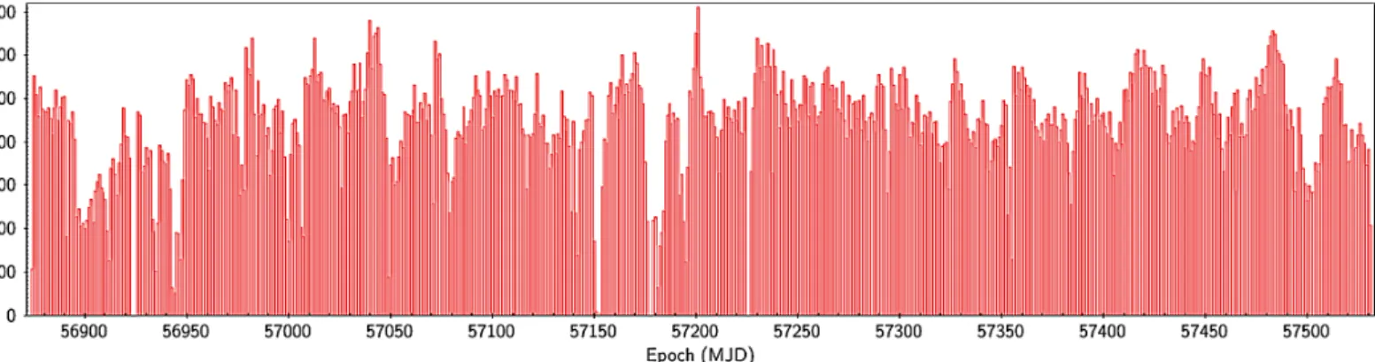
The general distribution of the observations is rather homo- geneous in time, with very rare gaps, in general shorter than a few hours; these are due to maintenance operations (orbital maneuvers, telescope refocusing, micrometeoroid hits, and other events; Fig.2).
A more detailed view of the distribution with a resolution of several minutes (Fig.3) reveals a general pattern that repeats at each rotation of the satellite (6 h) and is dominated by a sequence of peaks that correspond to the crossing of the ecliptic region by the two FOVs, at intervals of∼106 min (FOV 1 to FOV 2) and
∼254 min (FOV 2 to FOV 1). The peaks are strongly modulated in amplitude by the evolving geometry of the scan plane with respect to the ecliptic.
The observation dates are given in barycentric coordinate time (TCB) Gaia-centric3, which is the primary timescale for Gaia, and also in coordinated universal time (UTC) Gaia- centric. Timings correspond to mid exposure, which is the instant of crossing of the fiducial line on the CCD by the photocentre of the SSO image.
The accuracy of timing is granted by a time-synchronisation procedure between the atomic master clock onboard Gaia (providing onboard time, OBT) and OBMT, the onboard mis- sion timeline (Gaia Collaboration 2016). OBMT can then be converted into TCB at Gaia. The absolute timing accuracy requirements for the science of Gaia is 2 µs. In practice, this requirement is achieved throughout the mission, with a significant margin.
2.3. Geometry of detection
The solar elongation is the most important geometric feature in Gaia observations of SSOs. By considering the intersection of the scan plane with the ecliptic, as shown in Fig.5, it is clear that SSOs are always observed at solar elongations between 45◦and 135◦.
This peculiar geometry has important consequences on solar system observations. The SSOs are not only observed at non- negligible phase angles (Fig. 12), in any case never close to the opposition, but also in a variety of configurations (high/low proper motion, smaller or larger distance, etc.), which have some influence on many scientific applications and can affect the detection capabilities ofGaia and the measurement accuracy.
The mean geometrical solar elongation of the scan plane on the ecliptic is at quadrature. In this situation, the scan plane is
3 Difference between the barycentric JD time in TCB and 2455197.5.
Fig. 2.Distribution in time of the SSO observations published in DR2. The bin size is one day.
Fig. 3. Detail over a short time interval of the distribution shown in Fig.2.
Fig. 4.Geometry of theGaia NSL on the celestial sphere, with ecliptic north at the top. The scanning motion ofGaiais represented by the red dashed line. The precession of the spin axis describes the two cones, aligned on the solar–anti-solar direction, with an aperture of 90◦. As a consequence, the scan plane, here represented at a generic epoch, is at any time tangent to the cones. When the spin axis is on the ecliptic plane,Gaia scans the ecliptic perpendicularly, at extreme solar elon- gations. The volume inside the cones is never explored by the scan motion.
Fig. 5.By drawing the intersection of the possible scan plane orien- tations with the ecliptic, in the reference rotating around the Sun with theGaia spacecraft, the two avoidance regions corresponding the the cones of Fig.4emerge in the direction of the Sun and around opposi- tion. The dashed line represents the intersection of the scanning plane and the ecliptic at an arbitrary epoch. During a single rotation of the satellite, the FOVs ofGaia cross the ecliptic in two opposite directions.
The intersection continuously scans the allowed sectors, as indicated by the curved arrows.
inclined by 45◦ with respect to the ecliptic. During the preces- sion cycle, the scan plane reaches the extreme inclination of 90◦ on the ecliptic. In this geometry, the SSOs with low-inclination orbits move mainly in the AC direction when they are observed by Gaia. As the AC pixel size and window are approximately times larger than AL, the sensitivity to the motion in terms of flux loss, image shift, and smearing will thus be correspondingly lower.
These variations of the orientation and the distribution of the SSO orbit inclinations translate into a wide range of possible ori- entations of the velocity vector on the (AL, AC) plane. Even for a single object, a large variety of velocities and scan directions is covered over time.
2.4. Errors and correlations
The SSO apparent displacement at the epoch of each observa- tion is clearly a major factor affecting the performance ofGaia,
Fig. 6.Approximate sketch illustrating the effects of the strong differ- ence between the astrometry precision in AL (reaching sub-mas level) and in AC (several 100 s mas). The approximate uncertainty ellipse (not to be interpreted as a 2D Gaussian distribution) is extremely stretched in the AC direction. The position angle (PA) is the angle between the declination and the AC direction.
even within a single transit. Other general effects acting on single CCD observations exist, such as local CCD defects, local point spread function (PSF) deviations, cosmic rays, and background sources. For all these reasons, the exploitation of the single data points must rely on a careful analysis that takes both the geomet- ric conditions of the observations and appropriate error models into account.
A direct consequence of the observation strategy employed by Gaia is the very peculiar error distribution for the single astrometric observation.
Because of the AC binning, most accurate astrometry in the astrometric field for most observations is only available in the AL direction. This is a natural consequence of the design principle of Gaia, which is based on converting an accurate measurement of time (the epoch when a source image crosses a reference line on the focal plane) into a position. In practical terms, the difference between AC and AL accuracy is so large that we can say that the astrometric information is essentially one-dimensional.
As illustrated in Fig.6, the resulting uncertainty on the posi- tion can be represented by an ellipse that is extremely stretched in the AC direction. When this position is converted into another coordinate frame (such as the equatorial reference α, δ), a very strong correlation appears between the related uncertainties σα, σδ. Therefore it is of the utmost importance that the users take these correlations into account in their analysis. The values are provided in the ESA Archive and must be used to exploit the full accuracy of theGaiaastrometry and to avoid serious misuse of theGaia data.
3. Outline of the data reduction process
The solar system pipeline (Fig.7) collects all the data needed to process the identified transits (epoch of transit on each CCD, flux, AC window coordinates, and many auxiliary pieces of information).
A first module, labelled “Identification” in the scheme, com- putes the auxiliary data for each object, and assigns the iden- tifying correct identification label to each object. Focal plane coordinates are then converted into sky coordinates by using the transformations provided by AGIS, the astrometric global iterative solution, and the corresponding calibrations (astromet- ric reduction module). This is the procedure described below in Sect. 3.1. We note that this approach adopts the same princi- ple as absolute stellar astrometry (Lindegren et al. 2018): a local
Fig. 7.Main step of the solar system pipeline that collects all the data needed to process identified transits.
information equivalent to the usual small–field astrometry (i.e.
position relative to nearby stars) is never used.
Many anomalous data are also rejected by the same mod- ule. The post-processing appends the calibrated photometry to the data of each observation (determined by an independent pipeline, see Sect.4) and groups all the observations of a same target. Eventually, a “Validation” task rejects anomalous data.
The origin of the anomalies are multiple: for instance, data can be corrupted for technical reasons, or a mismatch with a nearby star on the sky plane can enter the input list. Identify- ing truly anomalous data from peculiarities of potential scientific interest is a delicate task. Most of this article is devoted to the results obtained on the general investigation of the overall data properties, and draws attention to the approaches needed to exploit the accuracy of Gaia and prepare a detailed scientific exploitation.
3.1. Astrometric processing
We now describe the main steps of the astrometric processing. A more comprehensive presentation is available in theGaiaDR2 documentation andLindegren et al.(2016,2018). The basic pro- cessing of the astrometric reduction for SSOs consists of three consecutive coordinate transformations.
The first step in the processing of the astrometry is the com- putation of the epoch of observations, which is the reconstructed timing of crossing of the central line of the exposure on the CCD.
The first coordinate transformation is the conversion from the Window Reference System (WRS) to the Scanning Reference System (SRS). The former consist of pixel coordinates of the SSO inside the transmitted window along with time tagging from the On Board Mission Timeline (OBMT), the internal time scale ofGaia(Lindegren et al. 2016). The origin of the WRS is the ref- erence pixel of the transmitted window. The SRS coordinates are expressed as two angles in directions parallel and perpendicular to the scanning direction ofGaia, and the origin is a conventional and fixed point near the centre of the focal plane ofGaia.
The second conversion is from SRS to the centre-of-mass reference system (CoMRS), a non-rotating coordinate system with origin in the centre of mass ofGaia.
The CoMRS coordinates are then transformed into the barycentric reference system (BCRS), with the origin in the barycentre of the solar system. The latter conversion pro- vides the instantaneous direction of the unit vector from Gaia to the asteroid at the epoch of the observation after removal of the annual light aberration (i.e., as if Gaia were station- ary relatively to the solar system barycenter). These positions, expressed in right ascension (α) and declination (δ), are provided in DR2. They are similar to astrometric positions in classical ground-based astrometry.
A caveat applies to SSO positions concerning the relativis- tic bending of the light in the solar system gravity field. In Gaia DR2, this effect is over–corrected by assuming that the target is at infinite distance (i.e. a star). In the case of SSOs at finite distance, this assumption introduces a small discrepancy (always<2 mas) that must be corrected for to exploit the ultimate accuracy level.
3.2. Filtering and internal validation
An SSO transit initially includes at most nine positions, each cor- responding to one AF CCD detection (see Sect.2). However, in many cases, fewer than nine observations in a transit are avail- able in the end. The actual success of the astrometric reduction depends on the quality of the recorded data: CCD observations of too low quality are quickly rejected; the same holds true if an observation occurs in the close vicinity of a star or within too short a time from a cosmic ray event, the software fails to produce a good position.
These problems represent only a small part of all the possi- ble instances encountered in the astrometric processing, which has required an efficient filtering. Observations have been care- fully analysed inside the pipeline to ensure that positions that probably do not come from an SSO are rejected, as well as positions that do not meet high quality standards. We applied the filtering both at the level of individual positions and at the level of complete transits. We list the main causes of rejection below.
– Problematic transit data. The positions were rejected when some transit data were too difficult to treat or if they gave rise to positions with uncertain precision.
– Error-magnitude relation. Positions with reported uncertain- ties that were too large or too small for a given magnitude are presumably not real SSO detections, and they were discarded.
– No linear motion. At a solar elongation of more than 45◦, an SSO should show a linear motion in the sky during a single transit, where linear means that both space coordinates are linear functions of time. We considered all those positions to be false detections that did not fit the regression line to within the estimated uncertainties.
– Minimum number of positions in a transit. The final check was to assess how many positions were left in a transit. For GaiaDR2, we set the limit to two because we relied on an a priori list of transits to be processed (see Sect.2.1).
SSOs have also gone through a further quality check and filtering according to internal processing requirements estab- lished to take into account some expected peculiarities of SSO signals.
Three control levels were implemented:
– Standard window checking. Only centroids/fluxes from windows with standard characteristics were accepted and transmitted to the following step of the processing pipeline.
– Checking of the quality codes in the input data, result- ing from the signal centroiding. Only data that successfully passed the centroid determination were accepted.
– A filtering depending on the magnitude and apparent motion of the source and the location of its centroid inside the window in order to reject observations with centroids close to the window limits, where the interplay between the distortion of the PSF due to motion and the signal trunca- tion would introduce biases in centroid and flux measure- ments.
3.3. Error model for astrometry
Between CCD positions within a transit, the errors are not entirely independent, since in addition to the uncorrelated ran- dom noise, there are some systematics, like the attitude error, that have a coherence time longer than the few seconds interval between two successive CCDs. This induces complex correla- tions between the errors in the different CCDs from the same transit that are practically impossible to account for rigorously.
Hence, we adopted a simplified approach separating the error into a systematic and a random part. Systematic errors are the same for all positions of the same transit, while random errors are statistically independent from one CCD to another. One of the main error sources is the error from the centroiding. It is propa- gated in the pipeline down from the signal processing in pixels in the coordinate system (AL, AC), and it is eventually converted into right ascension and declination. The errors in AL and AC are usually uncorrelated, but the rotation from the system (AL, AC) to the system (αcosδ,δ) makes them highly correlated.
Along-scan uncertainties are very small (of the order of 1 mas), and they show the extreme precision ofGaia. The error on the centroiding represents the main contribution to the ran- dom errors for SSOs fainter than magnitude 16. For SSOs fainter than magnitude 13, all pixels are binned in AC to a single win- dow, and the only information we have is that the object is inside the window. Therefore the position is given as the centre of the window, and the uncertainty is given as the dispersion of a rect- angular distribution over the window. The errors in AC are thus very large (of the order of 600 mas) and highly non-Gaussian.
For SSOs brighter than magnitude 13, the uncertainty in AC is smaller. In these cases, a 2D centroid fitting is possible, but the error in AC is generally still more than three times larger than in AL direction, essentially because of the shape of theGaiapixels.
An important consequence is that uncertainties given in the (αcosδ,δ) coordinate system may appear to be large as a result of the large uncertainties in AC, which contributes to the uncer- tainty in both right ascension and declination after the coordinate transformation.
Other errors also affect the total budget, such as the error from the satellite attitude and the modelling errors that are due to some corrections that are not yet fully calibrated or implemented.
They contribute to both the random and the systematic error and are of the order of a few milliarcseconds.
4. Asteroid photometry inGaiaDR2
TheGaiaArchive provides asteroid magnitudes inGaiaDR2 in theG band (measured in the AF white band), for 52% of the observations. This fraction is a result of a severe selection that is described below.
Asteroids, due to their orbital motion, move compared to stellar sources on the focal plane ofGaia. Hence, it is possible that they can drift out of the window during the observations of the AFs. This drift can be partial or total, resulting in potential loss of flux during the AF1, . . . ,AFx with x>1 observations.
Asteroid photometry at this stage is processed with the same approach as is used for stellar photometry (Carrasco et al. 2016;
Riello et al. 2018) and no specific optimisation is currently in place to account for flux loss in moving sources. This situation is expected to improve significantly in the futureGaia releases.
The photometry of Gaia DR2 is provided at transit level:
the brightness values (magnitude, flux, and flux error) repeat identically for each entry of the Gaia archive that is associ- ated with the same transit. The transit flux is derived from the
Fig. 8.Relative error in magnitudeσG for the whole sample of transit- levelGvalues. The vertical line atσG∼0.1 represents the cut chosen to discard the data with low reliability.
average of the calibrated fluxes recorded in each CCD strip of the AF, weighted by the inverse variance computed using the sin- gle CCD flux uncertainties. This choice minimises effects that are related, for instance, to windows that are off-centred with respect to the central flux peak of the signal. However, when the de-centring becomes extreme during the transit of a mov- ing object, or worse, when the signal core leaves the allocated window, significant biases propagate to the value of the transit average and increase its associated error. This happens in par- ticular for asteroids whose apparent motion with respect to stars is non-negligible over the transit duration. A main-belt asteroid with a typical motion of 5 mas s−1drifts with respect to the com- puted window by several pixels during the≈40s of the transit in theGaia FOV.
As provided by the photometric processing, a total of 234 123 transits of SSOs have an associated, fully calibrated magnitude (81% of the total). Figure8 shows the distribution of the rela- tive error per transitσGof the whole dataset before filtering. We found out that the sharp bi-modality in the distribution correlates positively with transits of fast moving objects. For this reason, we decided to discard all transits that fell in the secondary peak of large estimated errorsσG>10% as they almost certainly cor- respond to fluxes with a large random error and might be affected by some (unknown) bias.
A second rejection was implemented on the basis of a set of colour indices, estimated by using the red and blue photometer (RP and BP), the two low-resolution slitless spectrophotome- ters. Again due to asteroid motion, the wavelength calibration of RP/BP can be severely affected, and this in turn can affect the colour index that is used to calibrate the photometry in AF. In future processing cycles, when the accurate information on the position of asteroids, produced by the SSO processing system, will become available to the photometric processing, we expect to have a significant improvement in the calibration of the low- resolution spectra and photometric data for these objects. After checking the distribution of the observations of SSOs on a space defined by three colour indices (BP-RP, RP-G, and G-BP), we decided to discard the photometric data falling outside a reason- able range of colour indices, corresponding to the interval (0.0, 1.0) for both RB-G and G-RP.
The two criteria above, based on the computed uncertainty and on the colour, are not independent. Most transits that were rejected due to poor photometry in the G band also showed colour problems, which proves that the two issues are related.
Both filtering procedures together result in the rejection of a rather large sample of 48% of the initial brightness measurements available. In the end, 52% of the the transits
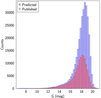
Fig. 9. Distribution of the apparent magnitude of the SSOs in Gaia DR2 at the transit epochs. For the whole sample the brightness derived from ephemerides (adopting the (H, G) photometric system) is provided (label: ”predicted”). The sub-sample contains the magnitude values that are published inGaiaDR2. The shift of the peak towards brighter values indicates a larger fraction of ejected values among faint objects.
Fig. 10.Distribution of the asteroid sample inGaiaDR2 as a function of solar elongation. The whole sample is compared to the sub-sample of asteroids with rejected photometric results (histogram of lower amplitude).
of SSOs inGaia DR2 have an associatedG-band photometry (Fig.9).
Figure10shows the difference in distribution of solar elonga- tion angles, between the entireGaiaDR2 transit sample and the transits for which the magnitude is rejected. Figure11shows the same comparison on the AL velocity distribution. The majority of rejections occurs at low elongations, where their average apparent velocity is higher.
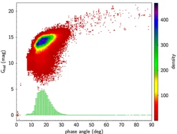
The resulting distribution of phase angles and reduced mag- nitudes (Gred, at 1 au distance fromGaia and the Sun) for the transits in Gaia DR2 is plotted in Fig. 12. In addition to the core of the distribution represented by MBAs, a small sample of NEAs reaching high phase angles is visible, as well as some transits associated with large TNOs at the smallest phase angles.
Fig. 11. Distribution of the asteroid sample inGaiaDR2 as a func- tion of AL velocity. The whole sample is compared to the sub-sample of asteroids with rejected photometric results (histogram of lower amplitude).
Fig. 12.Reduced asteroid magnitude as a function of phase angle. The histogram of phase angles is superposed on the bottom part (arbitrary vertical scale).
Despite the severe rejection of outliers, assessing the relia- bility of the published photometry at the expected accuracy of Gaia, specifically for solar system bodies, is not straightforward.
The intrinsic variability of the asteroids due to their changing viewing and illumination geometry and to their complex shapes makes the comparison of observed fluxes with theoretical ones very challenging. Sunlight scattering effects from the asteroid surfaces also play a role and must be modelled to reproduce the observed brightness.
We attempted to model the observed brightness following two different approaches, on a small sample of asteroids. First, we used a genetic inversion algorithm derived from a full inver- sion algorithm developed byCellino et al.(2009) and massively tested bySantana-Ros et al.(2015) to derive for a few selected objects the best–fitting three–axial ellipsoid (axis ratios) from Gaia observations alone. The procedure assumes known val- ues of the spin period and spin-axis direction (“asteroid pole”) available in the literature for objects that have been exten- sively observed from the ground, and takes into account a linear phase-magnitude dependence. The procedure is extensively explained in theGaiaDR2 documentation.
Independently, we exploited the detailed shape models avail- able for the two asteroids (21) Lutetia and (2867) Šteins derived by combining ground-based data with those obtained during the ESA Rosetta flybys to reproduce their observedGaiabrightness.
Both attempts, of course, concern modelling the flux variations relative to a given observation in the sample, not its absolute value.
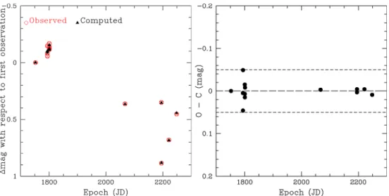
The results from the sparse photometry inversion are pre- sented in Figs.13–15. They are obtained by assuming a Lommel- Seeliger scattering law, a realistic choice when a more detailed mapping of the scattering properties across the surface is not available (Muinonen & Lumme 2015;Muinonen et al. 2015).
Despite the very simplified shape model, the residuals (observations minus computed) O-C are always within ±0.05 magnitudes, and the typical scatter can be estimated around 2–3%. Using the shape models of (21) Lutetia (Carry et al.
2010) and (2867) Šteins (Jorda et al. 2012), we tried to assess the photometric accuracy limit of Gaia on asteroids. In the case of (21) Lutetia, it was found that Gaia data are in very good agreement with expectations based upon the best available shape model of this asteroid, derived from disk-resolved imaging by Rosetta (which only imaged one hemisphere of the object) and a lower-resolution model based on disk-integrated, ground- based photometry. The high-resolution shape model reproduces the Gaia photometry with a small RMS value of 0.025 mag, corresponding to 2.3% RMS in flux. This strongly suggests thatGaiaphotometry is probably better than 2% RMS, within the limitations imposed by the shape model accuracy and the assumptions on the scattering model. Moreover,Gaiadata seem to offer an opportunity to improve the currently accepted shape solution for Lutetia, which is based partly upon ground-based data.
The results obtained for (2867) Šteins, for which a high- resolution shape model is also available, strongly support the conclusion that the photometry is indeed very accurate. For (2867) Šteins two pole solutions exist, essentially differing only by the value of the origin of the rotational phase. By directly using the shape model to reproduceGaiadata, resampled at 5◦ resolution, with a Lommel-Seeliger scattering corresponding to E-type asteroid phase functions, the RMS value of the O-C is 1.64% and 1.51% for the two pole solutions, a very good result.
Changing the resolution to 3◦ does not improve the fit further.
The remaining limitations in the case of (2867) Šteins are still related to details of the shape, and to the assumptions made (and/or scattering properties) when it was derived from Rosetta images.
In conclusion, our validation appears to show that Gaia epoch photometry, appropriately filtered to eliminate the out- liers, probably has an accuracy below 1–2% up to the magnitude of (2867) Šteins, in the range G 17-19. However, given the cur- rent limitations on the calibration and processing, we cannot exclude that the sample published in Gaia DR2 still contains a non-negligible fraction of anomalous data. For this reason, we recommend detailed analysis and careful checks for any applications based onGaiaDR2 photometry of asteroids.
5. Validation of the astrometry
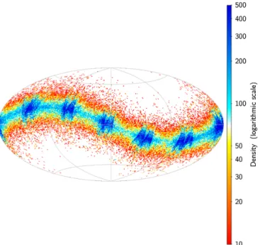
The processing of the solar system data described above has eventually produced a list with 14 124 objects (all numbered SSOs), 290 704 transits, and 2 005 683 CCD observations. The sky distribution is shown in Fig. 16 in a density plot in equatorial coordinates. As expected, most SSOs are found in a
Fig. 13.Observed and computed magnitude from the best fit ofGaiaobservations of an ellipsoidal model for the asteroid (39) Laetitia. In the right panel, we show the corresponding residuals. The origin of the time axis is J2010.0.
Fig. 14.As in Fig.13for the asteroid (283) Emma.
Fig. 15.As in Fig.13for the asteroid (704) Interamnia.
Fig. 16. Sky distribution (equatorial coordinates) of the 2 005 683 observations for the 14 124 asteroid in the validation sample. This sky map use an Aitoff projection in equatorial (ICRS) coordinates with α=δ=0 at the centre, north up, andαincreasing from right to left.
The observation density is higher in blue areas. The pattern in eclip- tic longitude is a consequence of theGaia scanning law over a small fraction of the five-year nominal mission.
limited range of ecliptic latitudes. The distribution in longitude is not uniform because over a relatively short duration of 22 months, theGaia scanning returned to the same regions of the sky, only in a limited number of areas.
Assessing the quality of the astrometry is challenging, and it needs an ad hoc treatment. Various filters have been applied during the activity of the astrometric reduction processing. The filtering process ensures the rejection of a maximum number of bad detections, while keeping the number of good positions that are rejected as small as possible (for more details, see the Gaia DR2 documentation). To prove that Gaia is already close to the performances expected at the end of the mission, we designed an ad hoc procedure for the external validation of the results. To this end, we fitted an orbit (initialising the fit with the best existing orbit) using only the available 22 months of Gaia observations, and we examined the residuals in right ascension and declination, and also in AL and AC (see Sect.5.1).
The main differences betweenGaia and ground-based observa- tions (or any other satellite observations) can be summarised as follows:
– Gaia observations are given in TCB, which is the primary timescale forGaia .
– Positions (right ascension and declination) are given in the BCRS as the direction of the unit vector from the centre of mass ofGaia to the SSOs.
– The observation accuracies are up to the order of few
∼10−9radians (sub-mas level) in the AL direction.
– The error model contains the correlations in αcosδ and δ because of the rotation from the (AL, AC) plane to the (αcosδ,δ) plane (Sect.3.3).
5.1. Orbit determination process
The orbit determination process usually consists of a set of math- ematical methods for computing the orbit of objects such as
planets or spacecraft, starting from their observations. For our validation purpose, we considered only the list of numbered asteroids for which the orbits were already well-known from ground-based (optical or radar)/satellite observations. We used the least-squares method and the differential correction algo- rithm (see Milani & Gronchi 2010) to fit orbits on 22 months ofGaia observations, using as initial guess the known orbits of these objects. To be consistent with the high quality of the data, we employed a high-precision dynamical model, which includes the Newtonian pull of the Sun, eight planets, the Moon, and Pluto based on JPL DE431 Planetary ephemerides4. We also added the contribution of 16 massive main-belt asteroids (see AppendixA).
We used a relativistic force model including the contribution of the Sun, the planets, and the Moon, namely the Einstein-Infeld- Hoffman approximation (Moyer 2003orWill 1993). As a result of the orbit determination process, we obtained for every object a corrected orbit fitted onGaiadata only together with the post-fit residuals.
The core of the least-squares procedure is to minimise the target function (Milani & Gronchi 2010),
Q= 1
mξTWξ, (1)
where m is the number of observations, ξ are the residu- als (observed positions minus computed positions), and W is the weight matrix. The solution is given by the normal equations,
C=BTW B; D=−BTWξ B=δξ δx
!
, (2)
where x is the vector of the parameters to be solved for. The differential corrections produce the adjustments∆xto be applied to the orbit:
∆x=C−1D.
It is clear from Eqs. (1) and (2) that the weight matrix plays a fundamental role in the orbit determination. It is usually the inverse of a diagonal matrix (Γ) that contains on the diagonal the square of the uncertainties in right ascension and declination for each observation, according to the existing debiasing and error models (as in Farnocchia et al. 2015). Each Gaia observation comes with its uncertainties on both coordinates and the correla- tion, which are key quantities in the orbit determination process.
Therefore the weight matrix in our case isW = Γ−1, where
Γ =
σ2α1 cov(α1, δ1) 0 · · · 0 cov(α1, δ1) σ2δ
1 0 · · · 0
... ... ...
0 0 · · · σ2αm cov(αm, δm)
0 0 · · · cov(αm, δm) σ2δm
.
The uncertainties used to build the W matrix are given by the random component of the error model, but we also take into account the systematic contribution when this is needed, as explained in the following section.
4 We also performed the orbit determination process using INPOP13c (Fienga et al. 2014) ephemerides and did not find significant differences in the results.
i
of the residuals for each observation, and γξ
i is the expected covariance of the residuals. Eachχ2i has a distribution of aχ2 variable with two degrees of freedom. We call outlier each obser- vation whoseχ2 value is greater than 25. The choice of 25 as a threshold was driven by the fact that we wished to keep as many good observations as possible and wished to discard only the observations (or the transits) that are very far from the expected Gaia performances. During this procedure, we took random and systematic errors into account.
Firstly, we rejected all the observations whoseχ2 value was greater than 25. Then, when the systematic part was larger than the random part, we performed a second step in the outlier rejection, described as follows:
– We computed the mean of the residuals for each transit.
– We checked if the value of the mean is lower than the systematic error for the transit.
– If the value was higher than the systematic error, we dis- carded the entire transit.
– If the value was lower than the systematic error, we com- puted for each observation the difference between the resid- ual and the mean value.
– We checked whether the difference was smaller than the ran- dom error. When that was the case, we kept the observation, otherwise we discarded it.
This approach is consistent with the uncertainties produced for GaiaDR2. Its underlying hypothesis is that the error correlations over a single transit can be completely represented by just one quantity, which is the value of the systematic component alone.
Although this is an approximation, we currently do not have the impression that a more complex correlation model is required.
5.3. Results
We fitted the orbits of the 14 124 asteroids contained in the vali- dation sample using an updated version of the OrbFit software5, developed to handle Gaia observations andGaia error model (Sects.5.1and5.2).
We were unable to fit the observations to the existing orbit for only three asteroids because the time span covered by the avail- able transits was too short. They were removed from the final output ofGaiaDR2. We also removed 22 bright objects (transits withG<10) whose residuals were substantially larger than the uncertainties we expected, and we considered these solutions as not reliable.
Figure 17 shows the distribution in semi-major axis and eccentricity of the 14 099 SSOs published in Gaia DR2. We can distinguish the NEA population (q <1.3) from the MBAs (including Jupiter trojans in this class) and the TNOs (q>28).
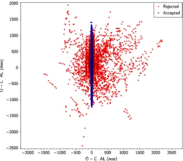
The total number of fitted observations is 2 005 683, which corresponds to 290 704 transits. During the outlier rejection pro- cedure (Sect.5.2), we discarded 27 981 observations (∼1% of the total). Figure18shows all the residuals in the (AL, AC) plane in
5 http://adams.dm.unipi.it/orbfit/
Fig. 17.Distribution of the 14 099 asteroids published inGaiaDR2 in semi-major axisa(au) and eccentricitye. The sample shows that all the broad categories of SSOs are represented (NEAs, MBAs, Jupiter trojans, and TNOs).
Fig. 18.Residuals in the (AL, AC) plane in milliarcseconds. Outliers are marked in red, while the blue thick line in the middle contains all the residuals for the accepted observations. The total number of fitted observations is 2 005 683, and there are 27 981 outliers (∼1% of the total).
mas. Outliers are the red points, while accepted observations are all contained in the blue thick line in the centre of the figure.
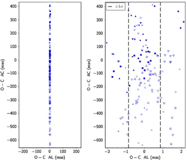
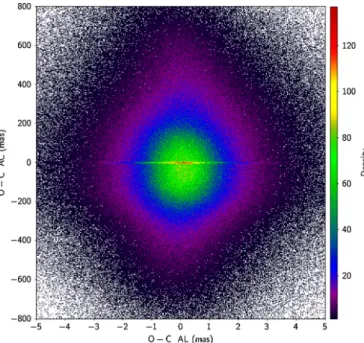
After the filtering and the outlier rejection,GaiaDR2 con- tains 1 977 702 observations, corresponding to 14 099 SSOs and 287 904 transits. Figure19represents a density plot of the resid- uals at CCD level in the (AL, AC) plane, for all the observations published in Gaia DR2. This plot, together with the plots of the residuals (Figs.20and21), shows the epoch-making change brought about byGaia astrometry: 96% of the AL residuals fall in the interval [–5, 5] mas and 52% are at sub-milliarcsecond

![Fig. 20. Left: AL residuals with respect to G magnitude. Right: Histogram of the AL residuals in the interval [–10,10] mas](https://thumb-eu.123doks.com/thumbv2/9dokorg/1395858.116457/14.892.99.800.124.447/left-residuals-respect-magnitude-right-histogram-residuals-interval.webp)