Dipper-like variability of the Gaia alerted young star V555 Ori

(1)

Dipper-like variability of the Gaia alerted young star V555 Ori

Zsófia Nagy,

¹^★

Elza Szegedi-Elek,

¹

Péter Ábrahám,

¹^,²

Ágnes Kóspál,

¹^,²^,³

Attila Bódi,

¹^,²^,⁴

Jérôme Bouvier,

⁵

Mária Kun,

¹

Attila Moór,

¹^,²

Borbála Cseh,

¹

Anikó Farkas-Takács,

¹

Ottó Hanyecz,

¹

Simon Hodgkin,

⁶

Bernadett Ignácz,

¹

Csaba Kiss,

¹^,²

Réka Könyves-Tóth,

¹

Levente Kriskovics,

¹^,²

Gábor Marton,

¹^,²

László Mészáros,

¹

András Ordasi,

¹

András Pál,

¹

Paula Sarkis,

³

Krisztián Sárneczky,

¹

Ádám Sódor,

¹

László Szabados,

¹

Zsófia Marianna Szabó,

¹^,⁷

Róbert Szakáts,

¹

Dóra Tarczay-Nehéz,

¹^,⁴

Krisztián Vida,

¹

Gabriella Zsidi

¹

1Konkoly Observatory, Research Centre for Astronomy and Earth Sciences, Eötvös Loránd Research Network (ELKH), H-1121 Budapest, Konkoly Thege Miklós út 15-17., Hungary

2ELTE Eötvös Loránd University, Institute of Physics, Pázmány Péter sétány 1/A, H-1117 Budapest, Hungary 3Max Planck Institute for Astronomy, Königstuhl 17, D-69117 Heidelberg, Germany

4MTA CSFK Lendület Near-Field Cosmology Research Group 5Univ. Grenoble Alpes, CNRS, IPAG, F-38000 Grenoble, France 6Institute of Astronomy, Madingley Road, Cambridge CB3 0HA, UK

7Eötvös Loránd University, Department of Astronomy, Pázmány Péter sétány 1/A, H-1117 Budapest, Hungary

Accepted XXX. Received YYY; in original form ZZZ

ABSTRACT

V555 Ori is a T Tauri star, whose 1.5 mag brightening was published as aGaiascience alert in 2017. We carried out optical and near-infrared photometric, and optical spectroscopic observations to understand the light variations. The light curves show that V555 Ori was faint before 2017, entered a high state for about a year, and returned to the faint state by mid-2018. In addition to the long-term flux evolution, quasi-periodic brightness oscillations were also evident, with a period of about 5 days. At optical wavelengths both the long-term and short-term variations exhibited colourless changes, while in the near-infrared they were consistent with changing extinction. We explain the brightness variations as the consequence of changing extinction. The object has a low accretion rate whose variation in itself would not be enough to reproduce the optical flux changes. This behaviour makes V555 Ori similar to the pre-main sequence star AA Tau, where the light changes are interpreted as periodic eclipses of the star by a rotating inner disc warp. The brightness maximum of V555 Ori was a moderately obscured (𝐴_𝑉=2.3 mag) state, while the extinction in the low state was𝐴_𝑉=6.4 mag. We found that while theGaiaalert hinted at an accretion burst, V555 Ori is a standard dipper, similar to the prototype AA Tau. However, unlike in AA Tau, the periodic behaviour was also detectable in the faint phase, implying that the inner disc warp remained stable in both the high and low states of the system.

Key words: Stars: variables: T Tauri – stars: pre-main sequence – Individual: V555 Ori

1 INTRODUCTION

Classical T Tauri stars are low-mass pre-main sequence objects sur- rounded by a circumstellar disc. These stars are still accreting ma- terial from the disc via magnetic field lines. Variability is a characteristic of young stars. Flux changes of a few tenth of a magnitude are typically caused either by rotating stellar spots or fluctuating accretion, producing periodic or irregular light curves, respectively.

Large amplitude brightening may also be present in the light curves when the accretion rate increases by several orders of magnitude due to thermal or gravitational instabilities in the disc, or perturba- tions by planets or close companions. This enhanced accretion rate causes outbursts in the optical light curve (Herbig 1977; Hartmann &

Kenyon 1996). Based on observations, these eruptive stars are tradi-

★ E-mail: nagy.zsofia@csfk.org

tionally divided into two classes: FU Orionis objects (FUors; several decades long outburst, absorption spectrum), and EX Lupi type objects (EXors, several months long repetitive outbursts, emission line dominated spectrum).

Deep fadings are also detected in light-curves of pre-main sequence variables. The intermediate-mass UX Orionis stars (UXors) show days to weeks long eclipse-like dimming at optical wavelengths, which are likely due to discs, where dense dust clumps within an or- biting rim at the inner edge of the disc may cross the line of sight and occult the star temporarily (Dullemond et al. 2003). Similar eclipse phenomena were identified among low-mass T Tauri stars, too. The AA Tau-like variables, or dippers, show periodic dips in their light curves, caused by eclipses of an inner disc warp main- tained by a tilted magnetic field (Bouvier et al. 1999, Bouvier et al.

2013). Since the brightness variations in young stars are related to the disc, infrared variability is also seen. Understanding the cause of the

arXiv:2103.10313v2 [astro-ph.SR] 24 Mar 2021

(2)

optical-infrared brightness variations provides unique information on the innermost part of the system.

One of the most efficient monitoring programmes to discover stars (including pre-main sequence stars) with large brightness variations is the Gaiaalerts system. In 2017 January aGaiaalert was published for the pre-main sequence star V555 Ori, whose brightness increased by 1.5 mag. The source is in the Orion star forming region, at aGaia-based distance of 388±12 pc (Bailer-Jones et al. 2018).

Near-infrared photometric and spectroscopic measurements imply an effective temperature of 4300±480 K (K4 spectral type), and a significant line-of-sight extinction of𝐴_𝑉 =7.98 mag (Da Rio et al.

2016). With a K4 spectral type and broad H𝛼lines as a tracer of accretion (Table 1), it is a classical T Tauri star.

Following-up theGaiaalert, we carried out a comprehensive optical and near-infrared photometric monitoring of V555 Ori. In this paper we combine these data with archival near- and mid-infrared data to better understand the nature of V555 Ori and the nature of physical processes which affect its brightness. We explain the observations and data reduction in Sect. 2, present results on the light curves, colour variations, and the detected spectral lines in Sect. 3, discuss the results in Sect. 4, and summarise them in Sect. 5.

2 OBSERVATIONS AND DATA REDUCTION

TheGaia alert¹ reported a 1.5 mag brightening of V555 Ori (or Gaia17afn, RA(J2000)=05:35:08.71, Dec(J2000)=−04:46:52.32) on 2017 January 24. The timescale and the amplitude of the brightening suggested a potential EXor outburst. We downloaded multi-epoch GaiaG-band photometry from the alerts service webpage. Figure 1 shows theGaialight curve, covering with irregular cadence the time interval between 2015 February and 2020 October. We supplemented these data with measurements available in public databases, and with our own new observations.

2.1 Follow-up optical photometry Photometric observations in the𝐵𝑉 𝑅

C𝐼

Cbands spanning the time interval between 2017 January and 2020 January were performed.

We obtained optical imaging observations using the 60/90/180 cm Schmidt telescope at Konkoly Observatory (Hungary), starting from about a week after theGaiaalert. The Schmidt telescope is equipped with a 4096×4096 pixel Apogee Alta U16 CCD camera (pixel scale:

1.03⁰⁰). Images were obtained in blocks of three frames per filter, and were reduced in IRAF.²After bias-, dark subtraction, and flat- fielding, aperture photometry was performed on each image using the IRAF ’phot’ task. The instrumental magnitudes were transformed into the standard system using the Fourth U.S. Naval Observatory CCD Astrograph Catalog (UCAC4) (Zacharias et al. 2013). The photometric errors were derived from quadratic sums of the formal errors of the instrumental magnitudes and the coefficients of the transformation equations. The results are shown in Table A1.

V555 Ori was also observed in the𝑉, 𝑅

C, and 𝐼

C bands with A Novel Dual Imaging CAMera (ANDICAM) installed on the SMARTS 1.3 m telescope at Cerro-Tololo Inter-American Obser- vatory (CTIO), in Chile. The CCD for the ANDICAM is a Fairchild

1 http://gsaweb.ast.cam.ac.uk/alerts/alert/Gaia17afn/

2 IRAF is distributed by the National Optical Astronomy Observatories, which are operated by the Association of Universities for Research in Astron- omy, Inc., under cooperative agreement with the National Science Foundation.

447 2k×2k chip. Bias and flat correction for the optical images were made by the Yale SMARTS team. The measured𝑉,𝑅

C, and𝐼

C

brightnesses are presented in Table A2. The photometric errors were derived from quadratic sums of the formal errors of the instrumental magnitudes of the comparison stars and those of the coefficients of the transformation equations.

2.2 Follow-up infrared photometry

Near-infrared,𝐽 𝐻 𝐾_𝑆measurements of V555 Ori were obtained using the ANDICAM dual-channel imager on SMARTS. The infrared (IR) detector was a Rockwell 1k×1k HgCdTe “Hawaii” array, used with 2×2 binning, with 0.⁰⁰276/pixel binned scale and 2.⁰4×2.⁰4 field of view. We used the CIT/CTIO𝐽 𝐻 𝐾_𝑆IR filters. A five-point dither- ing was made to enable bad pixel removal and sky subtraction in the IR images. Calibration was performed using the 2MASS magnitudes of 2–3 bright stars in the field of view. The typical photometric ac- curacy was about 0.02–0.03 mag in all three bands. These numbers were computed as the error of the mean of the distribution of the individual calibration factors, derived for the different comparison stars at different dither positions. The results are presented in Table A2.

2.3 Publicly available photometric observations

To reconstruct the light curve of V555 Ori before and after theGaia alert we supplemented our data with photometric data available in public databases.

We used data from the Zwicky Transient Facility (ZTF), which is a time-domain survey that had first light at Palomar Observa- tory in 2017. ZTF uses a camera with a 47 square degree field of view mounted on the Samuel Oschin 48-inch Schmidt telescope. We downloaded𝑔and𝑟 magnitude series of V555 Ori from the ZTF archive.³

V555 Ori was observed by the Transiting Exoplanet Survey Satel- lite (TESS, Ricker et al. 2015), for 23 days between 2018 mid- December and 2019 early January, as a part of the Sector 6 observ- ing run. The uninterrupted light curve had a cadence of 30 minutes.

We retrieved the full-frame images from the Mikulski Archive for Space Telescopes (MAST) and analysed them using a FITSH-based pipeline (Pál 2012) providing convolution-based differential imaging algorithms and subsequent photometry on the residual images.

Because the spectral sensitivity of the TESS detectors are close to the𝐼

Cband filter, we used our contemporaneous Schmidt𝐼

Cband data for the absolute calibration of the TESS photometry.

We used near-infrared JHK observations of V555 Ori obtained in 2000 March with the 2MASS telescope in Cerro Tololo. While the average value and the dispersion of the photometric measurements were published in Carpenter et al. (2001), we could also obtain the single epoch data points (J. Carpenter, private communication).

V555 Ori was monitored with theSpitzerspace telescope in the IRAC1 (3.6𝜇m) and IRAC2 (4.5𝜇m) bands, in the framework of the YSOVAR programme (Morales-Calderón et al. 2011). The observations were performed between 2009 Oct 23 and Dec 1, in the post-cryogenic phase of the mission.

NASA’s Wide-field Infrared Survey Explorer (WISE, Wright et al.

2010) mapped the whole sky at 3.4, 4.6, 12, and 22µm (W1, W2, W3, W4) in 2010 with an angular resolution of 6.1⁰⁰, 6.4⁰⁰, 6.5⁰⁰, and 12.0⁰⁰, respectively. After the depletion of the frozen hydrogen the survey continued as NEOWISE, later as NEOWISE-Reactivated

3 https://irsa.ipac.caltech.edu/Missions/ztf.html 000

(3)

3

6500 7000 7500 8000 8500 9000 9500

JD−2450000 19

18 17 16 15 14

Magnitude

Gaia DR2 G SMARTS Schmidt

ZTF

Pan−STARRS

W1+10 W2+10

2014 2016 2018 2020

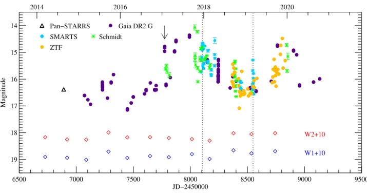
Figure 1.A combined𝑅-band optical light curve of V555 Ori between 2014 and 2020. Purple circles show magnitudes obtained in theGaia𝐺filter, whose spectral response is close to that of the Cousins𝑅_𝐶-band. The black triangle shows an average𝑅

Cvalue obtained from the Pan-STARRS survey, after converting from𝑟and𝑔magnitudes. Light blue and green symbols show the𝑅

Cdata points measured with the SMARTS and Schmidt telescopes, respectively. Data points from the ZTF survey displayed with orange symbols were converted to𝑅

Cmagnitudes from the original𝑔and𝑟values. To show the behaviour of the source at mid-infrared wavelengths, we overplotted the WISE data with blue and red diamonds. These data points are shifted as marked in the figure. Vertical dashed lines mark the epochs when the optical spectra were taken. The arrow marks theGaiaalert.

period using the two shortest wavelength detectors. For each WISE epoch, we downloaded all time resolved observations from the All- WISE Multiepoch Photometry Table and from the NEOWISE-R Single Exposure Source Table in the W1 (3.4 µm) and W2 (4.6 µm) photometric bands, and computed their seasonal average after removing outlier data points.

2.4 Optical spectroscopy

We observed V555 Ori using the Fiber-fed Extended Range Optical Spectrograph (FEROS) mounted at MPG/ESO 2.2m telescope at the European Southern Observatory (ESO) in La Silla, Chile. FEROS is a cross-dispersed échelle spectrograph that works in a fixed configu- ration and delivers continuous spectral coverage in the∼3500−9200 wavelength range with a spectral resolution of𝑅 =48 000 (Kaufer et al. 1999). Two spectra were taken on 2017 December 17 in object–

sky mode (i.e., the two fibers simultaneously recorded the science target and the sky background), and two spectra were taken on 2019 March 6 and 9 in object–calibration mode (when the two fibers simultaneously recorded the science target and the signal from a ThAr+Ne lamp). All four spectra were taken with 1800 s exposure time.

We reduced the FEROS spectra using a modified version of the ferospipe pipeline (Brahm et al. 2017) in python. The original pipeline has been developed to precisely measure the radial velocity of stars using cross correlation technique. To do so, it traces and extracts all the 33 available échelle orders, but calibrates only 25 of them, excluding eight orders that cover the∼6730−8230 Å range.

As this range contains several useful spectral features to study the accretion processes, we modified the code to expand the wavelength coverage. We identified the emission lines in the corresponding ThAr

spectra, which are used to carry out the new wavelength calibration.

The pipeline fits polynomials to the previously identified pixel value–

wavelength pairs in each order to iteratively sigma clip the outliers.

Then, these cleaned orders are fitted simultaneously using Chebyshev functions to improve the precision of the wavelength solution. To fit the pixel value–wavelength pairs in the newly added orders, we tested a wide range of coefficients and picked the ones where the standard deviation of the residual was approximately the same as if only the last 25 orders were used. Unfortunately, in the first 2 orders the low number of features in the ThAr spectra prevented us from a reliable line identification, thus we still had to exclude the∼8230−9000 Å range.

3 RESULTS 3.1 Light curves

Figure 1 shows a combined long-term R-band light curve of V555 Ori, usingGaiaG, Pan-STARRS, Schmidt𝑅

C, SMARTS𝑅

C, and ZTF𝑅

Cdata. The Pan-STARRS and ZTF𝑅

Cmagnitudes were converted from the original𝑔and𝑟magnitudes, using the formulae from Tonry et al. (2012). The optical light curve is supplemented by mid-infrared WISE photometry.

Figure 1 shows that already before theGaiaalert in 2017 Jan- uary, V555 Ori showed optical light variations, as typical for young stars. The source brightened about one magnitude during the year preceding the alert, and stayed in a bright state for about 200 days.

During 2018, the brightness of V555 Ori showed a decreasing trend, while continuously producing light variations. In early 2019 a sec-

(4)

8100 8110 8120 8130 JD−2450000

18 16 14 12 10

Magnitude

K_S H J

2017 Dec 5 −2018 Jan 8 I_C

R_C V

8152 8156

JD −2450000 2018 Feb 3−6

8180 8184

JD −2450000 2018 Mar 3−6

8211 8215

JD −2450000 18

16 14 12 10

Magnitude

2018 Apr 3−6

8434 8436 8438 8440 8442 8444 8446 8448 JD −2450000

2018 Nov 11−25

8544 8546 8548 8550 8552 8554 8556 JD −2450000

2019 Mar 2−13

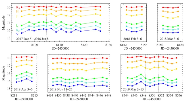
Figure 2.Subsets of the light curve measured in𝑉, R_C, I_C,𝐽,𝐻,andK_Scolours using the SMARTS telescope. The dotted lines mark the epochs of our optical spectroscopic observations.

8080 8100 8120 8140 8160 8180 JD−2450000

19 18 17 16 15 14

Magnitude

2017 Nov 25 − 2018 Feb 25 B

V R I

8385 8390 8395 8400

JD−2450000 19

18 17 16 15 14

Magnitude

2018 Sep 25 − Oct 10 B

V R I

Figure 3.Subsets of the light curve measured inB, V, R_C, andI_Ccolours using the Schmidt telescope.

ond brightening started, almost as high as in 2017, but somewhat shorter in time, and, according to the latest Gaiapoints, by mid 2020 V555 Ori became faint again. Interestingly, the mid-infrared light curves do not follow the optical trends, e.g. during the optical

8470 8475 8480 8485 8490

JD−2450000 17.5

17.0 16.5 16.0 15.5 15.0 14.5

Magnitude

Figure 4.TESS light curve of V555 Ori.

dimming in 2018 the WISE fluxes increased. The amplitude of the infrared variability is significantly lower than in the R-band.

Some limited parts of the light curve were sampled with an almost daily cadence. Photometry in theV, R_C, I_C, J, H, K_Sbands within these 2–3 weeks long periods between 2017 December and 2019 March are shown in Fig. 2. Similar plots for additional periods when only optical data were available, are displayed in Fig. 3. Finally, Fig. 4 shows the light curve obtained by TESS in 2018 December for a period of about 3 weeks. All these figures strongly suggest short term variability on the scale of a few days. The light curves also hint at a quasi-periodic behaviour, which will be further analysed in Sect. 3.3. Remarkably, the amplitude of the short-term variations is comparable to the amplitude of the long term trends.

000

(5)

5

0.5 1.0 1.5 2.0 B−V 17.5

17.0 16.5 16.0 15.5 15.0

V

0.0 0.5 1.0 1.5 V−R

0.0 0.5 1.0 1.5 R−I

7782 8050 8318 8586 8854

JD−2450000

1.0 1.2 1.4 1.6 1.8 2.0 J−H 10.2

10.0 9.8 9.6

KS

8095 8248 8402 8556 JD−2450000

0.40 0.45 0.50 0.55 IRAC1 − IRAC2 8.8

8.7 8.6 8.5

IRAC1

5130 5140 5150 5160 JD−2450000

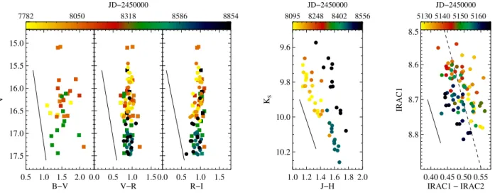
Figure 5.Left and middle panels:Colour−magnitude diagrams based on the optical and near-infrared data. Squares and circles show data measured with the SMARTS and Schmidt telescopes, respectively. The extinction paths correspond to𝑅_𝑉=5.5 and𝐴_𝑉=2 mag.Right panel:Colour−magnitude diagram based on theSpitzerIRAC1 and IRAC2 colours from the YSOVAR (Morales-Calderón et al. 2011) programme. The extinction path corresponds to𝑅_𝑉 =5.5 and 𝐴𝑉 =2 mag. A linear fit to the data points is shown with a dashed line.

0.8 1.0 1.2 1.4 1.6 1.8 10.2

10.0 9.8 9.6 9.4

KS

1998 Mar 19

− 2000 Apr 6 2MASS

0.8 1.0 1.2 1.4 1.6 1.8 2017 Dec 5

− 2018 Jan 8

0.8 1.0 1.2 1.4 1.6 1.8 2018 Feb 3

− 2018 Feb 6

0.8 1.0 1.2 1.4 1.6 1.8 J−H 2018 Mar 3

− 2018 Mar 6

0.8 1.0 1.2 1.4 1.6 1.8 2018 Apr 3

− 2018 Apr 6

0.8 1.0 1.2 1.4 1.6 1.8 2018 Nov 11

− 2018 Nov 25

0.8 1.0 1.2 1.4 1.6 1.8 2019 Mar 2

− 2019 Mar 13

Figure 6.J–H vs KScolour–magnitude diagrams and the extinction paths corresponding to𝑅_𝑉=5.5 and𝐴_𝑉=3 mag for the SMARTS data shown in Fig. 2, and for earlier data from Carpenter et al. (2001) and from 2MASS.

3.2 Colour variations

In Figure 5 we show the colour–magnitude diagrams based on our new optical and near-infrared data, as well as onSpitzerIRAC1 (3.6 𝜇m) and IRAC2 (4.5𝜇m) archival data from 2009. The epoch of the observations is colour-coded. In the optical (left panels), while the V vs. B–V plot exhibits relatively large scatter, which is probably due to measurement uncertainties in the B-band, the V vs. V–R and V vs. R–I figures reveal invariable colours over the whole∼2 mag brightness range. These constant colours do not seem to depend on the measurement date either.

At near-IR wavelengths (middle panel) there is a linear trend in the distribution of the data points that is approximately parallel to the extinction path. However, a cloud of points is also present above the main trend. In order to investigate them, Fig. 6 presents separate plots for the shorter periods displayed in Fig. 2. In general, the variability within each period is consistent with the reddening path based on Cardelli et al. (1989). They seem, however, to be slightly displaced from each other by various magnitudes either in the K^𝑆brightness or in the J–H colour, suggesting that additional physical processes may also contribute to the light variability. For comparison, we also plotted earlier data from 1998–2000 (left panel), which seem to be consistent with our new observations, and imply that during the

2MASS measurement the source was in an intermediate brightness state, while later, during the campaign of Carpenter et al. (2001), there were epochs when the system was as faint in the K^𝑆band as the minimum state in our observations in 2018 November. TheSpitzer IRAC data are shown in Fig. 5 (right panel). Due to the scatter seen in the data, we applied a linear fit to compare it to the extinction path.

The slope of the line which fits the data is 3.6±0.9, while the slope of the extinction path at the IRAC1 and IRAC2 wavelengths is 3.2, therefore the data are also consistent with changing extinction toward the source.

The presented optical–infrared colour–magnitude diagrams re- vealed different trends of V555 Ori in different spectral domains:

gray flux changes in the optical and extinction-like variations in the infrared. The possible explanation for this behaviour will be discussed in Sect. 4.

3.3 Frequency analysis

As seen in Fig. 2, the light curves in the different photometric bands are very similar, and they all show light variations on a time-scale of a few days. In order to characterise the virtually periodic nature of this variability, we performed a Lomb-Scargle periodogram analysis,

(6)

0.1 0.2 0.3 0.4 0.5 Frequency

0.0 0.2 0.4 0.6 0.8 1.0 1.2 1.4

Normalized LS Power

TESS 2018 Dec − 2019 Jan SMARTS 2017 Dec − 2018 Jan SMARTS 2018 Nov

SMARTS 2019 Mar

9 8 7 6 5 4Period (days)3 2

Figure 7.Lomb-Scargle periodograms based on the TESS data shown in Fig.

4 (black solid line), and the SMARTS V-band magnitudes observed in 2017 December - 2018 January (black dashed line), November 2018 (blue line), and March 2019 (red line).

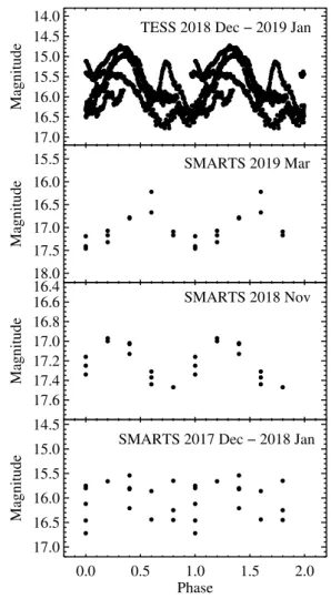
using the public tools at the NASA Exoplanet Archive Periodogram Service⁴. First we used the𝑉−band photometric sequence, obtained with the SMARTS instrument and shown in Fig. 2, to derive the most significant periods in the datasets for three epochs: 2017 Dec 5 to 2018 Jan 8; 2018 Nov 11 to 2018 Nov 25; and 2019 Mar 2 to 2019 Mar 13. Based on the periodogram results, the most significant periods in these datasets are close to 5 days, yielding 5.0±1.2 days and 4.8±1.4 days for the second and third SMARTS epochs, respectively. The periodogram corresponding to the first SMARTS epoch exhibits multiple periods, including a 4.7±0.3 day one. The difference between the periodogram results from first epoch compared to those from the other two may be related to the different time sam- pling of the data: the other two epochs were typically sampled with a daily cadence, while the 2017 Dec / 2018 Jan epoch was typically sampled with a 2-3 day cadence. We also calculated Lomb-Scargle periodogram for the TESS lightcurve (Fig. 4). The most significant period is 5.3±0.8 days, which is close to the result obtained from the SMARTS data. The errors of the periods were calculated by fit- ting Gaussian profiles to the peaks of the periodograms, and using half of the full width at half maximum (FWHM) values of the fitted Gaussians as the errors of the periods. The results are summarized in Fig. 7 and show the presence of a significant period around 5 days in both the TESS and SMARTS data. The light curves used for the frequency analysis folded in phase with a period of 5 days are shown in Fig. 8.

3.4 Optical spectra

The optical spectra analysed in this section represent the bright state (2017) and the faint state (2019) of V555 Ori. As mentioned before in Sect. 2.4, V555 Ori was measured in object–sky mode in 2017, but in object–calibration mode in 2019. The consequence of this is that the object spectra taken in 2019 are contaminated by thorium, argon, and neon lines from the calibration lamp. Therefore, when searching for emission lines in the spectra of V555 Ori, we only accepted as secure detection those lines that were present in the spectra both in 2017 and in 2019. Considering emission lines, we detected the H𝛼, H𝛽, H𝛾,

4 https://exoplanetarchive.ipac.caltech.edu/cgi-bin/Pgram/nph-pgram

17.0 16.5 16.0 15.5 15.0 14.5 14.0

Magnitude

TESS 2018 Dec − 2019 Jan

18.0 17.5 17.0 16.5 16.0 15.5

Magnitude

SMARTS 2019 Mar

17.6 17.4 17.2 17.0 16.8 16.6 16.4

Magnitude

SMARTS 2018 Nov

0.0 0.5 1.0 1.5 2.0

Phase 17.0

16.5 16.0 15.5 15.0 14.5

Magnitude

SMARTS 2017 Dec − 2018 Jan

Figure 8.The light curves used for the frequency analysis folded in phase with a period of 5 days.

and H𝛿lines of the hydrogen Balmer series, two forbidden ionized sulphur lines ([S ii] 671.8 nm and [S ii] 673.3 nm), two forbidden ionized nitrogen lines ([N ii] 655.0 nm and [N ii] 658.5 nm), and two forbidden neutral oxygen lines ([O i] 630.2 nm and 636.5 nm). We also detected one absorption line, that of Li i at 670.8 nm.

In order to flux-calibrate the spectra, we used optical photometry taken with the SMARTS or Piszkéstető Schmidt telescope on the same night as the spectrum in question. For the calibration of the spectra, we estimated the continuum flux of V555 Ori at each wavelength by interpolating in wavelength between the observed broad-band photometric points. Once the spectrum was in physical units, we fitted a linear continuum to the line-free channels on both sides of each line and subtracted it. The two spectra taken with a half hour difference in 2017 and the two spectra taken with three days difference in 2019 agreed within the uncertainties, therefore we averaged the two spectra for each year to increase the signal-to- noise ratio. The calibrated, continuum-subtracted, averaged spectra for the emission lines detected in V555 Ori can be seen in Fig. 9.

The difference between the noise levels at the two epochs, i.e., higher signal-to-noise ratio in 2019 than in 2017, is due to different weather conditions. During the 2017 observations, the humidity was close to 60%, the seeing was somewhat worse than 1 arcsec, while during 000

(7)

7

the 2019 observations, the humidity was about 40%, seeing slightly below 1 arcsec.

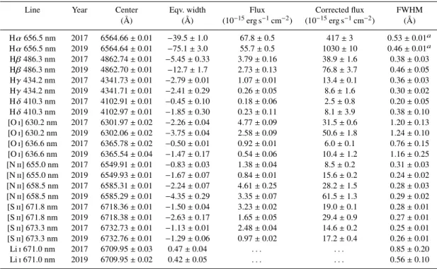
We used standard IRAF routines to measure the center location (or peak location for H𝛼), equivalent width, flux, and FWHM of the lines. These parameters, shown in Tab. 2, indicate that while the equivalent widths were typically larger in 2019 than in 2017, the lines fluxes decreased from 2017 to 2019. The explanation for this is that the continuum flux also decreased from 2017 to 2019, but with a larger factor than the line fluxes did. The equivalent width of the Li line did not vary noticeably, suggesting that the veiling did not change significantly between these two epochs.

Most emission lines we detected display simple Gaussian profiles.

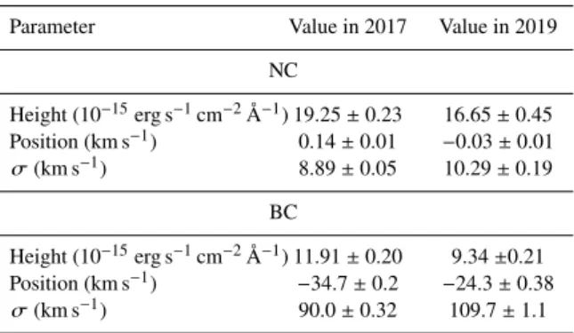
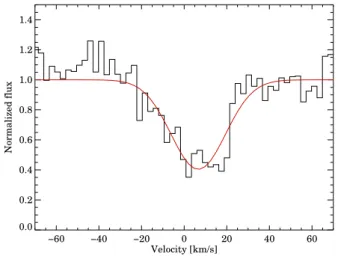
The only exception is H𝛼, which is more complex. In Fig. 10 we fitted the observed H𝛼profiles with the sum of two Gaussians, a narrow and a broad component (NC and BC). Tab. 1 shows the fitted parameters of the Gaussians in 2017 and 2019. The two Gaussians reproduce the profiles quite well, except for some extra absorption apparent between−85 km s⁻¹and−25 km s⁻¹in 2017 and between

−150 km s⁻¹ and−25 km s⁻¹ in 2019. The Gaussian width (𝜎) is on the order of 20 km s⁻¹ for the NC and 100 km s⁻¹ for the BC.

There is about 6 times more flux in the BC. While the NC appears at around the systemic velocity, the BC is blueshifted by −25 to

−35 km s⁻¹. The narrow component may be related to postshock gas and the broad component to the accretion flow (Hartmann et al. 2016 and references therein).

Fig. 9 and Tab. 2 show that the metallic emission lines became weaker in 2019 compared to 2017, but there are no discernible differences in the line profiles. We used the CHIANTI Database V 9.0⁵to calculate model line ratios for our observed lines for different𝑛_𝑒elec- tron densities and𝑇_𝑒electron temperatures (Dere et al. 1997, 2019).

For the observed [O i] and [N ii] lines, the line ratios do not depend on𝑛_𝑒or𝑇_𝑒, given that their upper levels are the same (Storey & Zeip- pen 2000), therefore we can simply compare the theoretical line ratio with the observed one. The theoretical line ratio for [O i] 630.2 nm / [O i] 636.5 nm is 3.13, while the measured ratios are 5.18±0.16 and 4.77±0.78 in 2017 and in 2019, respectively. The theoretical line ratio for [N ii] 655.0 nm / [N ii] 658.5 nm is 0.34, while the measured ratios are 0.29±0.03 and 0.25±0.01 in 2017 and in 2019, respectively.

Based on the observed ratios the lines are not saturated, i.e. they are optically thin, as otherwise the ratios would be closer to 1. The good agreement between the theoretical and observed line ratios for [N ii]

also suggests that they are formed in low-density gas, because the theoretical line ratios are valid in the low-density limit, otherwise collisional de-excitation would suppress these forbidden transitions.

The discrepancy for [O i] may be because of the uncertainty of the observed line ratio due to very low signal-to-noise detection of the [O i] 636.5 nm line. The [S ii] 671.8 nm / [S ii] 673.3 nm ratio de- pends both on 𝑛_𝑒 and𝑇_𝑒, given that the upper levels of the two transitions are different (Canto et al. 1980). The measured ratios are 1.30±0.02 and 1.70±0.04 in 2017 and in 2019, respectively. The model values typically give ratios above one for log(𝑛_𝑒)<2.5, while the ratio is below one for higher electron densities. We found no parameter combination to give a ratio larger than about 1.47. The largest ratios can be obtained for temperatures around 6000 K. The observed ratios suggest that the [S ii] lines are emitted by gas that has an electron density of 100 cm⁻³or less and temperature probably close to 6000 K. These values imply low ionization fraction and low temperature compared to typical values in jets of young stellar objects (𝑁

e∼10⁴cm⁻³and𝑇

e∼1.1−1.5×10⁴K, Gomez de Castro &

5 http://chiantidatabase.org/

Table 1.Parameters of Gaussian components fitted to the H𝛼lines of V555 Ori.

Parameter Value in 2017 Value in 2019

NC

Height (10⁻¹⁵erg s⁻¹cm⁻²Å⁻¹) 19.25±0.23 16.65±0.45 Position (km s⁻¹) 0.14±0.01 −0.03±0.01 𝜎(km s⁻¹) 8.89±0.05 10.29±0.19

BC

Height (10⁻¹⁵erg s⁻¹cm⁻²Å⁻¹) 11.91±0.20 9.34±0.21 Position (km s⁻¹) −34.7±0.2 −24.3±0.38

𝜎(km s⁻¹) 90.0±0.32 109.7±1.1

Pudritz 1993). On the other hand, the values of V555 Ori are higher compared to characteristic values of photodissociation regions (few cm⁻³and∼1000 K, Hollenbach & Tielens 1997). These may point to a weak disc wind in V555 Ori, with C-shocks rather than J-shocks (Hollenbach 1997).

4 DISCUSSION

4.1 Long-term variability: obscuration or outburst?

Fig. 1 demonstrates that V555 Ori underwent long-term brightness variations, including the∼1.5 magnitude brightening corresponding to theGaiaalert in early 2017, followed by a high state of∼200 days, a dimming to reach a minimum around late 2018 - early 2019, and a rise again in early 2020. These flux changes may be caused by variable circumstellar extinction and/or fluctuations in the accretion rate. In the following, we will quantify the changes in visual extinction based on the photometric data, then in the accretion rate based on our spectroscopic data.

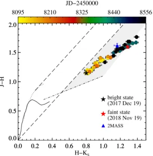
To measure the visual extinction in different brightness states of the long-term evolution, we analysed the location of the source in the near-infrared colour–colour diagram (Fig. 11). In order to separate the long-term trends from short-term quasi-periodic variability, we scrutinised the light curves in Fig. 2, and visually identified all epochs corresponding to maximum brightness of the∼5 day periodicity.

We assume that at these phases no extinction component related to the short-term variability affects the system’s apparent magnitude.

Among these peak epochs, we found that at infrared wavelengths V555 Ori was brightest on 2017 December 19, and faintest on 2018 November 19.

Using the expression from Cardelli et al. (1989), we measured the visual extinction of the source in the brightest epoch by projecting its location in Fig. 11 to the line representing the locus of unreddened T Tau stars (Meyer et al. 1997) along the extinction path. This method gives𝐴_𝑉=2.3 mag, which may largely be the interstellar reddening in the direction of the source. To determine the extinction in the faintest state, we measured the J–H difference magnitude between the brightest and faintest data points in Fig. 11 (black and red aster- isks, respectively), and converted it to A^𝑉 using the extinction law of Cardelli et al. (1989). We assumed an𝑅_𝑉of 5.5, as suggested by Da Rio et al. (2016) as an average value for the Orion A cloud. Adding to this value the bright state extinction of 2.3 mag, this approach resulted in 6.4 mag for 2018 November 19. Thus, we conclude that the long-term infrared variations of V555 Ori can be explained by changing extinction along the line-of-sight, whose value varies be-

(8)

−100 0 100

−1.0

−0.5 0.0 0.5 1.0 1.5 2.0

Hδ 410.3 nm

2017 2019

Fλ (10−15 erg s−1 cm−2 A−1)

−100 0 100

−2

−1 0 1 2 3 4

Hγ 434.2 nm

−100 0 100

−4

−2 0 2 4 6 8 10

Hβ 486.3 nm

−200 0 200

−10 0 10 20 30

Hα 656.5 nm

−50 0 50

0 5 10

[SII] 671.8 nm

−50 0 50

−2 0 2 4 6 8

[SII] 673.3 nm

−50 0 50

−1 0 1 2 3 4

[NII] 655.0 nm

−50 0 50

Velocity (km s⁻¹)

−5 0 5 10 15

[NII] 658.5 nm

−50 0 50

−1 0 1 2 3 4

[OI] 630.2 nm

−50 0 50

−1 0 1 2 3 4

[OI] 636.6 nm

Figure 9.Emission lines detected in the FEROS optical spectra of V555 Ori in 2017 December (red) and in 2019 March (blue).

Table 2.Parameters of the lines detected in V555 Ori. The FWHM values are uncorrected for the instrumental line broadening.

Line Year Center Eqv. width Flux Corrected flux FWHM

(Å) (Å) (10⁻¹⁵erg s⁻¹cm⁻²) (10⁻¹⁵erg s⁻¹cm⁻²) (Å) H𝛼656.5 nm 2017 6564.66±0.01 −39.5±1.0 67.8±0.5 417±3 0.53±0.01^𝑎 H𝛼656.5 nm 2019 6564.64±0.01 −75.1±3.0 55.7±0.5 1030±10 0.46±0.01^𝑎 H𝛽486.3 nm 2017 4862.74±0.01 −5.45±0.33 3.79±0.16 38.9±1.6 0.38±0.03 H𝛽486.3 nm 2019 4862.70±0.01 −12.7±1.7 2.73±0.13 76.8±3.7 0.46±0.05 H𝛾434.2 nm 2017 4341.73±0.01 −2.79±0.01 1.07±0.01 13.4±0.1 0.36±0.03 H𝛾434.2 nm 2019 4341.71±0.01 −2.41±0.29 0.26±0.05 8.6±1.6 0.30±0.02 H𝛿410.3 nm 2017 4102.91±0.01 −0.45±0.10 0.18±0.06 2.5±0.8 0.20±0.05 H𝛿410.3 nm 2019 4102.97±0.01 −1.85±0.30 0.23±0.11 8.1±3.9 0.38±0.10 [O i] 630.2 nm 2017 6301.97±0.02 −2.26±0.04 4.77±0.09 31.5±0.6 1.20±0.13 [O i] 630.2 nm 2019 6302.06±0.02 −3.75±0.04 2.58±0.09 50.6±1.8 1.24±0.10 [O i] 636.6 nm 2017 6365.78±0.02 −0.50±0.01 0.92±0.01 6.0±0.1 0.76±0.15 [O i] 636.6 nm 2019 6365.54±0.04 −1.47±0.17 0.54±0.06 10.4±1.2 1.16±0.25 [N ii] 655.0 nm 2017 6549.91±0.01 −0.83±0.03 1.38±0.04 8.5±0.2 0.31±0.03 [N ii] 655.0 nm 2019 6549.93±0.01 −1.67±0.07 0.84±0.01 15.6±0.2 0.24±0.02 [N ii] 658.5 nm 2017 6585.31±0.01 −2.24±0.07 4.61±0.25 28.2±1.5 0.28±0.03 [N ii] 658.5 nm 2019 6585.29±0.01 −4.35±0.29 3.35±0.07 61.5±1.3 0.29±0.02 [S ii] 671.8 nm 2017 6718.36±0.01 −1.50±0.04 3.23±0.02 19.0±0.1 0.28±0.01 [S ii] 671.8 nm 2019 6718.38±0.01 −2.63±0.17 1.65±0.05 29.4±0.9 0.27±0.01 [S ii] 673.3 nm 2017 6732.73±0.01 −1.13±0.01 2.48±0.04 14.6±0.2 0.25±0.01 [S ii] 673.3 nm 2019 6732.76±0.01 −1.29±0.06 0.97±0.02 17.2±0.4 0.26±0.01

Li i 671.0 nm 2017 6709.95±0.03 0.47±0.04 . . . . . . 0.85±0.20

Li i 671.0 nm 2019 6709.95±0.02 0.42±0.05 . . . . . . 0.56±0.10

𝑎FWHM of the narrow component.

tween A^𝑉=2.3 mag and 6.4 mag. The extinction-based interpretation is also supported by the the middle and right panels of Fig. 5.

Note, that at optical wavelengths the flux changes do not follow what would be expected from changing obscuration, whose possible explanations will be discussed in Sect. 4.3. Our A^𝑉value of 6.4 mag, obtained for the faintest state, is not far from the∼8.0 mag derived by Da Rio et al. (2016) for V555 Ori using the (J–H) colour. In Fig. 11, V555 Ori appears as a moderately reddened T Tau star, whereas in the faint state its near-infrared colours move to the right, beyond the

area occupied by reddened Class II young stellar objects (Meyer et al.

1997).

In addition to extinction, mass accretion from the circumstellar disc onto the star may also cause brightness variations. Based on our optical spectra obtained close in time to the brightest and the faintest epochs, we derived accretion rates from the flux of the H𝛼 line, taking its broad components as accretion tracer. The measured line flux values are presented in Tab. 2, but for our analysis they need to be corrected for extinction. Based on our previous result, for the 2017 December 17 spectrum (bright state) we adopted A^𝑉=2.3 mag 000

(9)

9

−200 0 200

−10 0 10 20 30

Fλ (10−15 erg s−1 cm−2 A−1) 2017 data

NC BC NC+BC

−200 0 200

2019 data

NC BC NC+BC

Figure 10.Profiles of the H𝛼line and Gaussian fits.

0.0 0.2 0.4 0.6 0.8 1.0 1.2 1.4 0.0

0.5 1.0 1.5 2.0

0.0 0.2 0.4 0.6 0.8 1.0 1.2 1.4 H−K_S

0.0 0.5 1.0 1.5 2.0

J−H

8095 8210 8325 8440 8556

JD−2450000

bright state (2017 Dec 19) faint state (2018 Nov 19) 2MASS

Figure 11.(J−H) vs. (H−KS) colour–colour diagram. The solid curve shows the colours of the zero-age main sequence, and the dotted line represents the giant branch (Bessell & Brett 1988). The long-dashed lines delimit the area occupied by the reddened normal stars (Cardelli et al. 1989). The dash-dotted line is the locus of unreddened T Tau stars (Meyer et al. 1997) and the gray shaded band borders the area of the reddened KS-excess stars. The coloured filled circles are SMARTS data, with their colours representing the date of the observations.

and used the standard extinction law of Cardelli et al. (1989). This calculation resulted in 4.2×10⁻¹³erg cm⁻²s⁻¹. Correcting the line fluxes in the faint state is less straightforward, since at these wavelengths the measured variability amplitude is lower than predicted by the extinction law, as seen in Fig. 12. Thus, using the A^𝑉=6.4 mag and the Cardelli et al. (1989) extinction law would over-predict the extinction corrected line flux of the H𝛼line. Instead, we will assume that the H𝛼line flux and the neighbouring continuum changed, due to extinction, by the same amount between the bright and faint epochs.

Taking advantage that our spectra are flux calibrated (Sect. 3.4), we determined a ratio of 3.0 between the continuum fluxes in the bright and faint spectra around 656 nm, and scaled up the H𝛼line flux measured in 2019 by this ratio. It yielded 1.0×10⁻¹²erg cm⁻²s⁻¹. Then we used the equations of Alcalá et al. (2014) to transform L_lineto Lacc, and finally to ˙Macc(adopting Mstar=1.1 M, and Rstar=3R).

1 log λ (µm) 0.0

0.5 1.0 1.5 2.0

Magnitude

2017 Dec, A_V=2.1 mag 2018 Nov, AV=0.7 mag 2019 Mar, A_V=3.1 mag 2017−2018, AV=4.1 mag

Figure 12.Magnitude differences between the minimum and maximum of the

∼5 day brightness variations in 2017 Dec (black), in 2018 Nov (green), and in 2019 Mar (red). The blue symbols show the difference between the brightness during outburst (2017 Dec) and quiescence (2018 Nov), and both correspond to the same phase (maximum) of the 5-day brightness variations. The visual extinctions corresponding to the𝐽,𝐻, and𝐾

Sdata and the extinction curves calculated using the formulae from Cardelli et al. (1989) are also shown.

140000 145000 150000 155000

−1 0 1 2

140000 145000 150000 155000

Upper level energy (K)

−1 0 1 2

log10(Nup / gup)

T_ex = 5800 K T_ex = 4600 K

2017 2019

Figure 13.Excitation diagram for hydrogen. The linear fits only use the H𝛼, H𝛽, and H𝛾lines.

The results are ˙Macc= 3.3×10⁻⁹Myr⁻¹and 8.8×10⁻⁹Myr⁻¹in 2017 December and in 2019 March, respectively.

Detecting several lines of the Balmer series (Sect. 3.4) allows us to determine the excitation temperature of the gas that emits these lines. First, we corrected the line fluxes in both the bright and faint states, following the procedure applied for the H𝛼line above. Then in Fig. 13 we plotted the relative level populations calculated in LTE approximation divided by the statistical weights of the energy levels in question in logarithmic scale as a function of the energy of the levels. The data point for H𝛿is quite uncertain, so we fitted only three data points, H𝛼, H𝛽, and H𝛾, with a straight line. The inverse of the slope of this line gave an excitation temperature of 5800 K in 2017

(10)

and 4600 K in 2019. These values are higher than the photospheric temperature of a K4-type star, indicating that the detected hydrogen lines originate from gas participating in the accretion process, located close to the magnetospheric hot spot, or residing in the accretion column. The excitation temperatures calculated above are similar to those calculated by Muzerolle et al. (1998b) in their magnetospheric accretion models. We also used Eqn. 9 from Hartmann et al. (2016) to calculate the effective temperature of the heated photosphere of V555 Ori. Assuming the average value of the derived accretion rates, and the result is∼5500 K.

The calculated accretion rate change would imply a change in the optical veiling, as these two quantities are expected to correlate well (e.g., Muzerolle et al. 1998a). However, the equivalent width of the Li absorption line was constant within the measurement uncertainties, suggesting constant veiling. This apparent contradiction can be resolved if we consider that the accretion luminosities calculated for 2017 Dec and 2019 Mar (Lacc=0.03 Land 0.08 L, respectively) are so low compared to the luminosity of the star, that the result- ing veiling (and its change) would remain below our detection limit (cf. Fig. 4 of Muzerolle et al. 1998a). Also, the luminosity changes caused by accretion variability would not be enough to explain the observed brightness variations of V555 Ori, leaving us with the most plausible interpretation that the light curves in Fig. 1 are related to changing obscuration along the line of sight rather than to accretion changes.

4.2 The circumstellar structure of V555 Ori

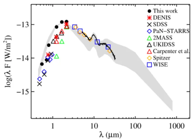
Based on the available photometric data and the reddening values determined in the previous subsection, we constructed the spectral energy distribution (SED) of V555 Ori over the 0.36−24µm wavelength range, as seen in Fig. 14. In addition to data collected from the literature, we also plotted the optical–infrared fluxes obtained by us at the date of the maximum brightness on 2017 December 19.

The large scatter in the optical and near-infrared parts is consistent with the large-amplitude variability analysed in this work. While the optical part is dominated by the reddened star, the shape of the SED at infrared wavelengths suggests the presence of a circumstellar disc.

TheSpitzerIRS spectrum also reveals broad 10𝜇m and 20𝜇m spectral features attributed to small silicate grains in the surface layer of the disc. In the figure we overplotted the “Taurus median”, which is based on the SEDs of T Tauri stars in the Taurus region (D’Alessio et al. 1999, Furlan et al. 2006). We reddened the Taurus median by 𝐴_𝑉=2.3 mag, as derived above for the bright state, and normalized it to the H-band flux of V555 Ori. The figure shows that the Taurus median is very similar to the measured SED, indicating that V555 Ori possesses a rather typical, average protoplanetary disc. While such discs are usually passive, i.e. powered mainly by irradiation from the central T Tauri star, a smaller contribution from the accretion process may also present.

4.3 The origin of the short-term variability

Based on observations carried out with SMARTS and TESS, we identified brightness variations with an amplitude of∼1 mag in V band on a time-scale of∼5 days. In order to determine the physical origin of this variability, in Fig. 12 we compared the multicolour magnitude differences corresponding to the short-term (∼5-day) and long term brightness variations, based on our SMARTS data in the𝑉,𝑅_𝐶,𝐼_𝐶, 𝐽,𝐻, and K^𝑆bands. The short-term brightness differences represent the magnitude change between the maximum and minimum of a se- lected∼5-day cycle. The plotted long-term variation corresponds to

1 10 100 1000

λ (µm)

−13

−14

2 log(λ F [W/m]) −15

This work DENIS SDSS PaN−STARRS 2MASS UKIDSS Carpenter et al.

Spitzer WISE

Figure 14.Spectral energy distribution of V555 Ori. The shaded area shows the ‘Taurus’ median SED reddened by the extinction of𝐴_𝑉=2.3 mag determined for the bright state and normalised to the H-band flux measured with SMARTS in the bright state (black circles). The data points below 1.25𝜇m and above 34𝜇m are from D’Alessio et al. (1999); otherwise from Furlan et al. (2006). The spectrum, obtained with the Infrared Spectrograph (IRS) ofSpitzerwas downloaded from the Combined Atlas of Sources withSpitzer IRS Spectra.

the difference between the brightest state (2017 December 19) and the faintest state (2018 November 19), and both correspond to the maximum phase of the 5-day brightness variations. The figure clearly demonstrates that the wavelength dependence of the short-term and long-term variations are indistinguishable. They differ only in their amplitudes, the short-term amplitudes being somewhat smaller. In all cases, the 𝐽, 𝐻, and 𝐾_𝑆 magnitude differences closely follow the standard extinction curve (overplotted in the figure). The optical magnitude differences, however, always smaller than predicted from the extinction curve matching the near-IR data points of the same date. Moreover, the optical changes show little wavelength dependence, as was already implied by the left panel of Fig. 5. One possible reason of the lower optical magnitude differences could be a significant scattered light contribution that originates from the outer disc regions. The presence of an invariable optical component would render any changes related to obscuration of a part of the system smaller on the magnitude scale. Our result strongly suggests that the brightness variations on both short and long time-scales are related to changing extinction. Given that the accretion luminosities are low (0.03-0.08𝐿) compared to the luminosity of V555 Ori (3.39𝐿), the short-term brightness variations of 1 mag - equivalent to a factor of 2.5 change in the luminosity - are unlikely to be affected by the accretion.

4.4 A twin of AA Tau?

Quasi-periodic variability, caused by changing extinction, is a defin- ing characteristics of the dipper class of variable low-mass young stellar objects. Brightness variations, similar to those observed in V555 Ori, were found earlier for AA Tau, the prototypical member of the dipper class: Bouvier et al. (1999) observed a∼8.5 day,∼1.4 mag quasi-periodic variability in the𝑈,𝐵,𝑉,𝑅, and𝐼filters. The be- havior of AA Tau was interpreted as periodic occultations of the star by an inner disc warp, and are likely driven by a misalignment between the stellar magnetic dipole and rotation axes (Bouvier et al.

000