Journal Pre-proofs

Journal Pre-proofs

Distance assessment and analysis of high-dimensional samples using varia‐

tional autoencoders

Marco Inacio, Rafael Izbicki, Bálint Gyires-Tóth

PII: S0020-0255(20)30653-8

DOI:

Reference: INS 15628

To appear in:

Received Date: 6 December 2019 Revised Date: 1 May 2020 Accepted Date: 29 June 2020

Please cite this article as: M. Inacio, R. Izbicki, B. Gyires-Tóth, Distance assessment and analysis of high- dimensional samples using variational autoencoders,

j.ins.2020.06.065

This is a PDF file of an article that has undergone enhancements after acceptance, such as the addition of a cover page and metadata, and formatting for readability, but it is not yet the definitive version of record. This version will undergo additional copyediting, typesetting and review before it is published in its final form, but we are providing this version to give early visibility of the article. Please note that, during the production process, errors may be discovered which could affect the content, and all legal disclaimers that apply to the journal pertain.

© 2020 Published by Elsevier Inc.

Distance assessment and analysis of high-dimensional samples using variational autoencoders

Marco Inacio^1,2,3, Rafael Izbicki³, Bálint Gyires-Tóth⁴

Abstract

An important question in many machine learning applications is whether two samples arise from the same generating distribution. Although an old topic in Statistics, simple accept/reject decisions given by most hypothesis tests are often not enough: it is well known that the rejection of the null hypothesis does not imply that differences between the two groups are meaningful from a practical perspective. In this work, we present a novel nonparametric approach to visu- ally assess the dissimilarity between the datasets that goes beyond two-sample testing. The key idea of our approach is to measure the distance between two (possibly) high-dimensional datasets using variational autoencoders. We also show how this framework can be used to create a formal statistical test to test the hypothesis that both samples arise from the same distribution. We evaluate both the distance measurement and hypothesis testing approaches on simulated and real world datasets. The results show that our approach is useful for data exploration (as it, for instance, allows for quantification of the discrepancy/sepa- rability between categories of images), which can be particularly helpful in early phases of the a machine learning pipeline.

Keywords: variational autoenconders; two-sample comparison;

high-dimensional data; hypothesis testing

1Corresponding author: m@marcoinacio.com.

2University of São Paulo.

3Federal University of São Carlos.

4Budapest University of Technology and Economics.

1. Introduction

An important question in many applications of machine learning and Statis- tics is whether two samples (or datasets) arise from the same data generating

probability distribution [gretton2012kernel,holmes2015two,soriano2015bayesian].

Although an old topic in statistics [Mann47,Smirnov48], simple accept/reject

5

decisions given by most hypothesis tests are often not enough: it is well known that the rejection of the null hypothesis does not mean that the difference be- tween the two groups is meaningful from a practical perspective [1904.06605, Wasserstein2019]. Thus, tests that go beyond accept/reject decisions are preferred in practice. In particular, tests that provide not only single and in-

10

terpretable numerical values, but also a visual way of exploring how far apart the datasets are from each other especially useful. This raises the question of how to assess the distance between two groups meaningfully, which is especially challenging in high-dimensional spaces.

In this work, we present a novel nonparametric approach to assess the dis-

15

similarity between two high-dimensional datasets using variational autoencoders (VAE) [vae]. We show how our approach can be used to visually assess how far apart datasets are from each other via a boxplot of their distances and addi- tionally, provide a way of interpreting the scale of these distances by using the distance between known distributions as a baseline. We also show how a formal

20

permutation-based hypothesis testing can be derived within our framework.

The remaining of this paper is organized as follows. In sections 1.1 and 1.2, we present a brief description of work related to our proposed method. In Section2, we present a review of variational inference and VAE, and show that the latter can be interpreted as a density estimation procedure, which is the basis

25

of the proposed method. In Section3, we show how variational autoencoders can be used as a method of exploring the differences between two samples. In Section 4, we use our method to derive a formal hypothesis testing procedure.

Both sections also show applications of the methods to simulated and real-world datasets. Finally, Section5concludes the paper with final remarks. Appendix5

30

contains details on the configurations of the software and neural networks used, as well as a link to our implementation, which is published open source.

1.1. Related work on two-sample hypothesis testing

Several nonparametric two-sample testing methods have been proposed in the literature; they date back toMann47,Smirnov48,WELCH1947: three

35

classical two-sample tests (Mann-Whitney rank test, Kolmogorov-Smirnov and Welch’s t-test, respectively) which were designed to work for univariate random variables only. On the other hand, holmes2015two, soriano2015bayesian, ceregatti2018wiksinvestigate Bayesian univariate methods for this task.

More recently,gretton2012kernelintroduce a two-sample test comparison

40

using reproducing kernel Hilbert space theory that works for high-dimensional data. The test, however, does not provide a way of to visually assess the dissim- ilarity between the datasets. two-sample-deep-learningproposes a method for two-sample hypothesis testing utilizing deep learning, which contrary to a permutation based test, only controls the type-1 error rate asymptotically;

45

binary-two-sampleproposes a test statistic built using binary classifier in the context of causal inference and causal discovery, also relaying on asymptotic dis- tribution for the test statistic (the distance between the performance of binary classifiers) under the null hypothesis.

Other two-sample tests for high-dimensional data can be found in [mondal2015high,

50

NIPS2016_6209] and references therein. Although these tests are robust and effective in many settings, they do not provide a visual analysis to assess the distance between the groups. Thus, they do not provide ways of checking if the difference between the datasets is meaningful from a practical perspective, a gap in literature which is filled by this article.

55

1.2. Related work on two-sample comparison and distance measurement There has also been some work devoted to two-sample comparison and re- lated tasks: In particular deAlmeidaIncio2018, provides a framework for assessing the distance between populations using density estimation methods.

However, the method provided in that work is based on MCMC (Markov Chain

60

Monte Carlo) Bayesian simulations, and therefore it is unable to scale to large datasets (seebetancourt_mcmc_subsampling, for instance) and high-dimensional spaces. In this work, we overcome these issues by using variational autoencoders to estimate densities, and by introducing a specific metric which has an analytic solution even in high-dimensional spaces).

65

pmlr-v97-kornblith19a (and references therein) proposes a new method of comparison of neural networks representation. pmlr-v48-larsen16propose a variant of variational autoencoders (VAE) that better measure similarities in data space than a vanilla VAE.an2015variationaluses VAEs for anomaly de- tection: that is, with the goal of identifying whether a single instance is different

70

from an observed sample. 1280752 evaluates existing similarity measurement methods in the context of image retrieval. These papers however do not use their methods for performing formal hypothesis tests.

Finally, for closely-related problems and applications, see alsopfister2016kernel, ramdas2017wasserstein,1908.00105for methods on how to solve the prob-

75

lem of independence testing anddesmistifying-gans which uses two-sample tests as a tool to evaluate generative adversarial networks.

2. Variational Autoencoders

In this section, we review key aspects of the variational autoencoders frame- work [vae] which are important to our proposed method.

80

Variable Autoencoders are among the most famous deep neural network ar- chitectures. The generative behaviour of VAEs makes these model attractive for many application scenarios. VAEs are often used in computer vision re- lated tasks. Introducing labeled data to the VAE training, attribute vectors, such as smile vector [yan2016attribute2image], can be computed; i.e. in

85

yan2016attribute2image the smile vector is computed by subtracting the mean latent vector for images of smiling and non-smiling people. In the gen- eration phase, this vector can be altered in the latent space to generate faces

with different smiling attributes. Another work utilizes VAEs to predict the possible movement of objects on images, pixelwise [walker2016uncertain].

90

Videos were also generated from text by combining VAEs with Generative Ad- versarial Network (GANS) [li2018video]. VAEs are also successfully applied in speech technologies. hsu2017learning learns latent representations from un- labelled data with VAEs for speech transformation (including phonetic content and speaker identity). In text-to-speech synthesis systems VAEs can be success-

95

fully applied for learning attributes and thus, controllable, expressive speech can be generated [akuzawa2018expressive]. Other types of sequences, like text, can also be modeled with VAEs. semeniuta2017hybrid uses convolutional encoder and deconvolutional decoder components, augmented with a recurrent language model in a variational autoencoder architecture to model text. Further-

100

more, there have been numerous theoretical research that focuses on or utilizes VAEs, like for second-order gradient estimation [fan2015fast], for importance weighting [burda2015importance], for anomaly detection [suh2016echo] and for novel architectures, like ladder VAE [sonderby2016ladder].

2.1. Statistical definition

105

Consider an i.i.d. random sample D = (X1, X2, ..., Xn). Variational au- toencoders estimate the density of this sample by encoding the information of each Xi using latent random variables Z = (Z1, Z2, ..., Zn), which are linked to (X1, X2, ..., Xn) by a parameter θ. More precisely, the model assumes the structure

Pθ(D=d|Z) = Yn

i=1

N(Xi=xi; (µi, σi) =gθ(Zi)),

where Zi ∼ N(0,1), gθ is a complex function (which is the output of a neu- ral network) with parameter θ (i.e.: the parameters/weights of a neural net- work), and µi and σi are the mean and standard deviation of the Gaussian distribution. Inference on such model is performed by maximizing the evidence P(D=d;θ) :=Pθ(D=d).

110

Note that, ifgθ is complex enough, we can actually model any distribution ofXi [devroye1986sample]. This is whygθis parametrized using an artificial neural network; it leads to flexibility (because of the richness of the space of functions they can represent,Hornik1989) as well as scalability.

Unfortunately, maximization of the evidence cannot be directly solved due

115

to the curse of dimensionality [tutorial_vae]. The next section shows how variational inference can be used to overcome this.

2.2. Variational inference

The curse of dimensionality can be solved using variational inference, which consists of optimizing

logPθ(D=d)−DKL(Q^(Z|D=d)_φ |P_θ^(Z|D=d))

=EQ_φ[logPθ(D|Z)|D=d]

−DKL(Q^(Z|D=d)_φ |P^(Z))

whereDKLrefers to the Kullback-Leibler divergence andQgiven by:

Qφ(Zi|Xi=xi) =N(Zi; (µi, σi) =hφ(xi))

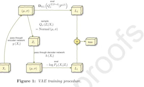
This framework is called variational autoenconder and it solves the curse of dimensionality [vae]. The training procedure for variational autoencoders is

120

presented in Figure1; for more details, seevae.

2.3. Generative model

The trained model can be used to generate new instances Xej: this can be done by applying Pθˆ(Xej) = R

Pθˆ(Xej|fZj = z)P^(Ze^j)(dz) , i.e.: sampleZ ∼ N(0,1), apply it on the neural network gθ and then sample from a N((µ, σ) =

125

gθ(z)). Therefore, variational autoencoders are a Gaussian⁵mixture model (of

5Note that variational autoencoders setup can be used with distributions other then Gaus- sians; e.g.: discrete data with Bernoulli distribution.

+ + loss pass though

encoder network

sample

pass though decoder network

eval eval

Figure 1: VAE training procedure.

an infinite number of Gaussians), and thus a density estimator.

2.4. Identifiability of the mixture of Gaussians

As per the structure of variational autoencoders, the distribution of such mix-

ture of Gausssians is not identifiable [teicher1961identifiability,wechsler2013bayesian]:

130

two different configurations of the parameters, say θ1 and θ2, can lead to the exact same distribution of(µ, σ). That is, gθ₁(Z)∼gθ₂(Z)even ifθ16=θ2.

In other words: if we train a variational autoencoders framework on a dataset, we will get a “generator” of pairs(µ, σ), saym1; and if we train a vari- ational autoencoders framework with identical structure on the same dataset,

135

we will get another “generator” of pairs (µ, σ), say m2. Generators m1 and m2 do not necessarily give the same distribution over samples of pairs (µ, σ).

Nonetheless, the induced final density (i.e., the Gaussian mixture) should be same analytically (i.e.: ignoring the stochastic variation that estimation meth- ods induce).

140

3. Two sample comparison: definition of the distance

We name our approach for assessing the similarity between two datasets, D1 andD2 asvaecompareand describe it as follows. First, we train two varia-

tional autoencoders: one forD1and one forD2. Letgθ₁ andgθ₂ be the learned functions for each of the autoencoders. gθ₁ andgθ₂, together withZ∼N(0,1), induce two distributions over the parameter space (µ, σ). Let S1 = (µ1, σ1) and S2 = (µ2, σ2) be two samples generated from the enconders gθ₁ and gθ₂, respectively. We then measure the distance between S1 and S2. Now, recall that each (µ, σ) is used to generate a new sample X ∼N(µ, σ) (Section 2.3).

Thus, a meaningful distance between S1 and S2 should be in the space of the random variables they generate. The key idea to make the method computa- tionally feasible is to use a symmetric Kullback-Leibler divergence between the distributions induced byS1andS2:

D(S1, S2) :=DKL(PS₁, PS₂) +DKL(PS₂, PS₁)

2d ,

wheredis the dimension of the feature space, PSi is a (multivariate) Gaussian distribution with parameters(µi, σi), and DKL is the Kullback-Leibler diver- gence. DKL has an analytical solution in the Gaussian case:

DKL(N(µ1, σ₁^TI),N(µ2, σ₂^TI)) = 1

2

2 Xd

i=1

logσ2,i−logσ1,i

!

−d

+ Xd

i=1

σ²_1,i/σ_2,i²

! +

Xd

i=1

σ_2,i² (µ2,i−µ1,i)²

! .

In case X represents an image, we use the standard approach of using multi-dimensional Bernoulli distributions with dimensions independent from each other (see [vae, tutorial_vae], for instance). In this case, the Kullback-

Leibler can also be obtained analytically:

DKL(Bernoulli(p),Bernoulli(q)) +DKL(Bernoulli(q),Bernoulli(p))

= Xd

i=1

(qi−pi)(log(qi)−log(pi) + log(1−pi)

−log(1−qi))

Using this approach, we can therefore assess the distance between one sample generated from the first autoencoder and a sample generated from the second autoencoder. In order to assess the divergence between the datasets D1 and D2, we can repeat this procedure several times; this will give a sample of the

145

distribution of distances.

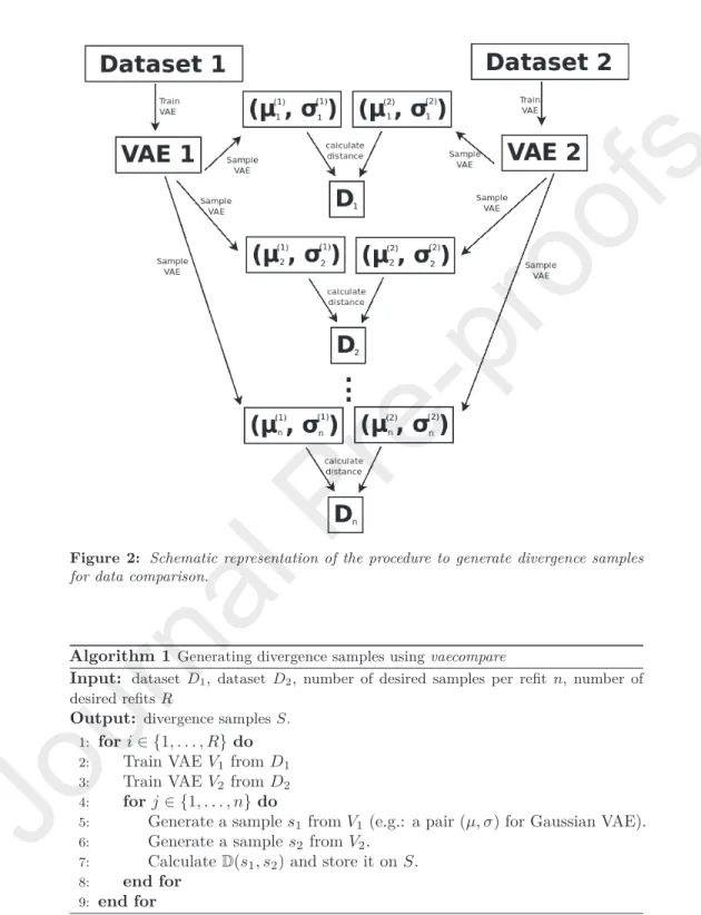
Now, in order to overcome the identifiability issue discussed in Section2.4, we train the variational autoencoders multiple times (we call these “refits”) for each dataset (using distinct initialization seeds for the network parameters) and use the new instances pairs(µ, σ)from each of them in equal proportion. The

150

full procedure is summarized in Algorithm1and Figure2.

Note that from the perspective of applying this method to images, it can also be interpreted as a data exploration tool, as it helps exploring the separa- bility and uncertainty of classes of images and the relation between their data generating processes.

155

3.1. Assessing the magnitude of the distance

In Section 3, we defined a method to measure the distance between two datasets. A yardstick is still required in order to say what is a “low” and “high”

distance. In order to create a baseline to interpret such distances, we proceed in similar fashion asdeAlmeidaIncio2018: we compute the distance between

160

two known distributions.

In the case of Gaussian VAEs we can work for instance with D(N0,N1), whereN0is a multivariate Gaussian with covariance given by an identity matrix

Figure 2: Schematic representation of the procedure to generate divergence samples for data comparison.

Algorithm 1Generating divergence samples usingvaecompare

Input: dataset D1, datasetD2, number of desired samples per refitn, number of desired refitsR

Output: divergence samplesS.

1: fori∈ {1, . . . , R}do

2: Train VAE V1 fromD1 3: Train VAE V2 fromD2 4: forj ∈ {1, . . . , n}do

5: Generate a samples1 fromV1 (e.g.: a pair(µ, σ)for Gaussian VAE).

6: Generate a samples2 fromV2.

7: CalculateD(s1, s2)and store it onS.

8: end for

9: end for

and mean given by a vector of zeros andN1 is a multivariate Gaussian with covariance given by an identity matrix and mean given by a vector of ones.

165

We have that D(N0,N1) = 1/2. For binomial VAEs, we use known binomial distributions as the baseline.

3.2. Evaluation (images)

Next, we apply the our method to CIFAR10 data [cifar10] using the VAE as a generator of binomial distributions. The dataset consists of images from

170

10 distinct categories (ranging from 0 to 9), with each category containing 5000 images. To make the comparison fair when comparing a category to itself and when comparing a category to another, we chose to work with half of each cat- egory dataset (2500 images) to train each VAE; i.e.: when comparing category 0 to category 1, one VAE is trained with 2500 images from category 0 and the

175

other is trained with 2500 images from category 1; on the other hand, when comparing category 0 to itself, each VAE is trained with half (2500 images) of the category 0 dataset. We worked with 90 VAE refits for each dataset.

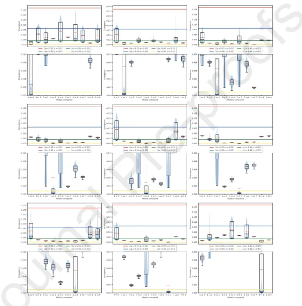
In Figure3, we present the results of such experiment with boxplots of the obtained divergences for all possible category combinations (note that the lower

180

image of each plot is a zoomed-in version of the upper image). The figure also shows the median and mean for each category, as well as the divergence of known Bernoulli distributions (plotted as horizontal lines).

Except for categories 0, 2 and 4, the divergence samples were all concentrated near zero when comparing a category to itself (a desirable behaviour). On the

185

other hand, for these 3 categories, we can observe a considerable amount of divergence samples spread far from zero indicating some uncertainty, but even in this case, there was a considerable amount of them near zero. Note also that the median for these three categories is much closer to zero than the mean, indicating its resilience to outliers.

190

On the other hand, when making comparisons between distinct categories, there are cases with high uncertainty (i.e.: boxplots with wide extensions; gen- erally with few points close to zero), as well as cases with higher certainty (i.e.:

Figure 3: Box plots of samples from our divergences comparing categories 0 to 8 to all categories. Note that the lower image of each plot is a zoomed-in version of the upper image.

boxplots with narrow extensions).

We conclude that the method is therefore useful for the purpose of data

195

exploration as it works as expected in a complex space such as images.

4. Hypothesis testing

We can additionally use vaecompare to directly test if two samples come from the same population. One way to do this is to find a threshold value (cutpoint) from a decision theoretic stand point where we would reject the null

200

hypothesis of the two samples coming from the same population. This is what is done in [ceregatti2018wiks] in the case of a Dirichlet process prior, where the threshold is chosen so as to control type I error of the hypothesis test.

Unfortunately, this is not possible in general and in general the cutpoint depends on the true data generating function.

205

Given that, we work instead with a simple permutation test where the datasets are repeatedly permuted against each other (i.e.: their data is mixed), and the average divergence of the samples is used as a test statistic. The p- value is then given by the quantile of the non-permuted dataset among all the statistics⁶. We note that for the hypothesis test to work in the sense of being a

210

proper test (uniform under the null), it is not necessary to do VAE refits, but refits increase the test power as we shall see next. We present the procedure in Algorithm2.

4.1. Evaluation (simulated data)

In this section, we apply the proposed hypothesis testing method to simu- lated datasets from a known data generating function and plot the observed p-value distribution. The data generating function for the datasets is defined

6For instance, if 43 of the permuted datasets had resulted on a lower divergence statis- tic than that of non-permuted dataset and on the other hand 57 had resulted on greater divergence, then the p-value would be43/(43 + 57) = 0.43.

Algorithm 2Obtaning the p-value for hypothesis testing usingvaecompare Input: dataset D1, datasetD2, number of desired samples per refitn, number of desired refitsR, number of permutations t, averaging functionM (e.g. mean or me- dian)

Output: p-valueρ.

1: fori∈ {1, . . . , t}do

2: Run Algorithm1, and store the results inSi.

3: Calculate M(Si)and store the result inKi.

4: Permute the instances of datasets D1 andD2.

5: end for

6: Obtain the number of points q1 in {K2, K3, ..., Kt} which are greater than K1.

7: Obtain the number of points q2 in {K2, K3, ..., Kt} which are greater than or equal toK1.

8: Setq= (q1+q2)/2

9: Store(q+ 1)/(t+ 1)inρ.

as:

lgr(µ=log(2), σ=α)−lgr(µ=log(2), σ= 0.5) +gr(µ= 1, σ= 2) +k

where lgr stands for multivariate log Gaussian random number generator, and gr

215

stands for multivariate Gaussian random number generator, both with diagonal covariance matrices. Moreover,α={0.2 + 0.7∗i/9}ⁱ⁼⁹_i=0, i.e.: αi= 0.2 + 0.7∗i/9 fori∈ {0,1, ...,9}.

For simplicity, we do not use refits here. The value of the vector k is fixed in zero for one of the datasets, and varied for the other. This is done in order

220

to change the dissimilarity between the samples (i.e.: the larger k is, the more dissimilar the sample distributions are) and from that, observe the behaviour of the distribution of the p-value.

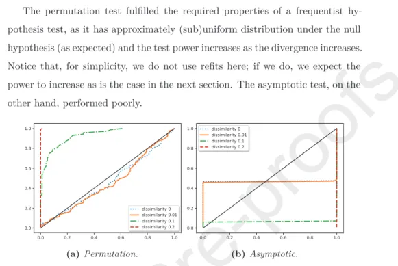
In Figure4a, we present the results of such experiment using the permutation test: the empirical cumulative distribution of the p-values; while in Figure4b,

225

we do the same simulation study using an Gaussian asymptotic approximate to the permutation test.

The permutation test fulfilled the required properties of a frequentist hy- pothesis test, as it has approximately (sub)uniform distribution under the null hypothesis (as expected) and the test power increases as the divergence increases.

230

Notice that, for simplicity, we do not use refits here; if we do, we expect the power to increase as is the case in the next section. The asymptotic test, on the other hand, performed poorly.

(a) Permutation. (b) Asymptotic.

Figure 4: Empirical cumulative distribution function of the p-values for distinct dis- similarity values (when the dissimilarity is zero, the null hypothesis is true) using a permutation test and asymptotic (approximate to permutation test).

4.2. Evaluation (images)

Here, we also applied the hypothesis testing method to the CIFAR10 dataset,

235

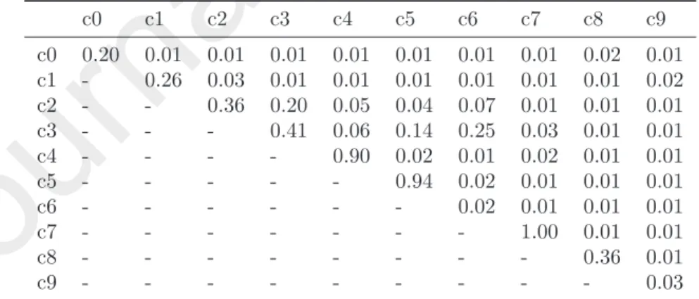
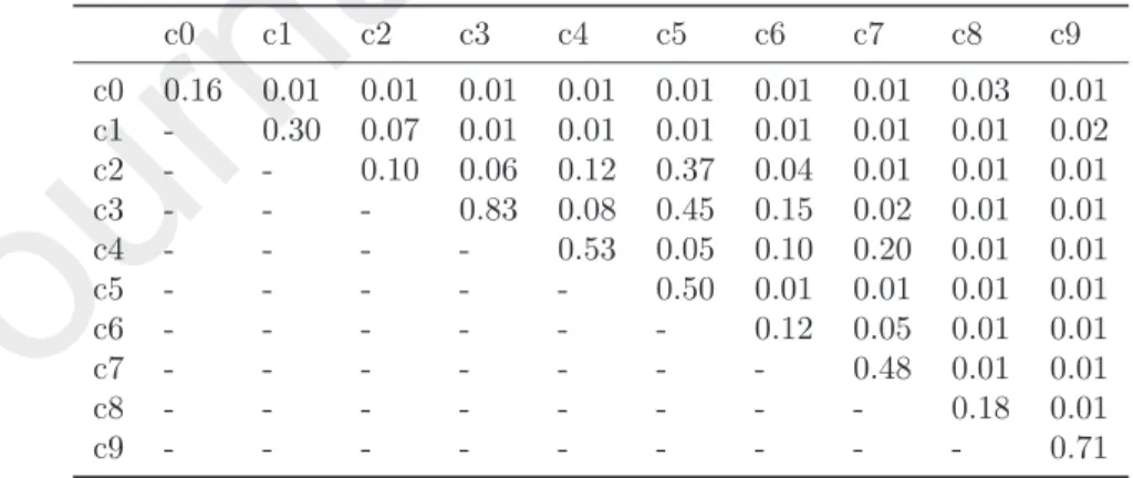
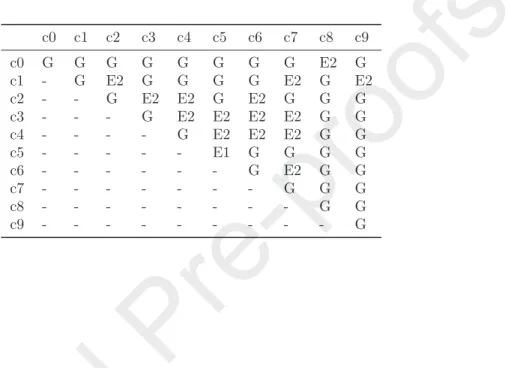
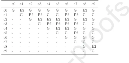
using the same 2500 images for each category as described in3.2. In Tables1,2, 3and4we present the p-values obtained in the test while in Tables5,6,7and 8we present the combinations that gave the correct results and type 2 error for a significance level of 5%. We applied the tests both without VAE refits and with 5 refits; we also tried the median as an alternative to the mean with the

240

intuition that this might help remove the weight of outlier distance points.

In Table9, we present a summary of the results. The method performed well under the null for both the mean and median metrics. Moreover, the method has shown to have a significant increase in test power when used with VAE refits.

245

In case of metrics performance comparison, it can be seem that the mean had incurred in less type I errors while the median incurred in larger but an admissible number given the critical rate of 5%. On the other hand the perfor- mance of median metric was considerably better regarding type II errors, this might be related to its robustness to outliers which have shown to be a frequent

250

problem in the Figure3.

Table 1: P-values for hypothesis testing for each categorywithoutrefits and averaging using themedian.

c0 c1 c2 c3 c4 c5 c6 c7 c8 c9

c0 0.99 0.01 0.01 0.01 0.01 0.01 0.01 0.01 0.40 0.01 c1 - 0.42 0.56 0.01 0.01 0.01 0.05 0.24 0.03 0.37 c2 - - 0.74 0.50 0.40 0.04 0.58 0.04 0.01 0.01

c3 - - - 0.78 0.31 0.26 0.49 0.22 0.01 0.01

c4 - - - - 0.39 0.21 0.29 0.23 0.01 0.01

c5 - - - 0.02 0.01 0.01 0.01 0.01

c6 - - - 0.96 0.32 0.01 0.01

c7 - - - 0.78 0.01 0.01

c8 - - - 0.06 0.01

c9 - - - 0.54

Table 2: P-values for hypothesis testing for each categorywith refits and averaging using themedian.

c0 c1 c2 c3 c4 c5 c6 c7 c8 c9

c0 0.20 0.01 0.01 0.01 0.01 0.01 0.01 0.01 0.02 0.01 c1 - 0.26 0.03 0.01 0.01 0.01 0.01 0.01 0.01 0.02 c2 - - 0.36 0.20 0.05 0.04 0.07 0.01 0.01 0.01

c3 - - - 0.41 0.06 0.14 0.25 0.03 0.01 0.01

c4 - - - - 0.90 0.02 0.01 0.02 0.01 0.01

c5 - - - 0.94 0.02 0.01 0.01 0.01

c6 - - - 0.02 0.01 0.01 0.01

c7 - - - 1.00 0.01 0.01

c8 - - - 0.36 0.01

c9 - - - 0.03

Table 3: P-values for hypothesis testing for each categorywithoutrefits and averaging using themean.

c0 c1 c2 c3 c4 c5 c6 c7 c8 c9

c0 0.25 0.12 0.01 0.01 0.01 0.01 0.01 0.01 0.48 0.05 c1 - 0.82 0.50 0.23 0.03 0.05 0.07 0.15 0.01 0.05 c2 - - 0.19 0.49 0.48 0.44 0.09 0.02 0.10 0.01

c3 - - - 0.22 0.11 0.36 0.15 0.27 0.01 0.01

c4 - - - - 0.87 0.20 0.40 0.01 0.01 0.01

c5 - - - 0.19 0.05 0.23 0.01 0.01

c6 - - - 0.73 0.01 0.01 0.01

c7 - - - 0.48 0.01 0.02

c8 - - - 0.45 0.06

c9 - - - 0.48

Table 4: P-values for hypothesis testing for each categorywith refits and averaging using themean.

c0 c1 c2 c3 c4 c5 c6 c7 c8 c9

c0 0.16 0.01 0.01 0.01 0.01 0.01 0.01 0.01 0.03 0.01 c1 - 0.30 0.07 0.01 0.01 0.01 0.01 0.01 0.01 0.02 c2 - - 0.10 0.06 0.12 0.37 0.04 0.01 0.01 0.01

c3 - - - 0.83 0.08 0.45 0.15 0.02 0.01 0.01

c4 - - - - 0.53 0.05 0.10 0.20 0.01 0.01

c5 - - - 0.50 0.01 0.01 0.01 0.01

c6 - - - 0.12 0.05 0.01 0.01

c7 - - - 0.48 0.01 0.01

c8 - - - 0.18 0.01

c9 - - - 0.71

Table 5: Results of the hypothesis testing when applying a critical rate of 5%without refits and averaging using themedian. Here G stands for “good” and E2 for type 2 error.

c0 c1 c2 c3 c4 c5 c6 c7 c8 c9

c0 G G G G G G G G E2 G

c1 - G E2 G G G G E2 G E2

c2 - - G E2 E2 G E2 G G G

c3 - - - G E2 E2 E2 E2 G G

c4 - - - - G E2 E2 E2 G G

c5 - - - E1 G G G G

c6 - - - G E2 G G

c7 - - - G G G

c8 - - - G G

c9 - - - G

Table 6: Results of the hypothesis testing when applying a critical rate of 5% with refits and averaging using themedian. Here G stands for “good” and E2 for type 2 error.

c0 c1 c2 c3 c4 c5 c6 c7 c8 c9

c0 G G G G G G G G G G

c1 - G G G G G G G G G

c2 - - G E2 G G E2 G G G

c3 - - - G E2 E2 E2 G G G

c4 - - - - G G G G G G

c5 - - - G G G G G

c6 - - - E1 G G G

c7 - - - G G G

c8 - - - G G

c9 - - - E1

Table 7: Results of the hypothesis testing when applying a critical rate of 5%without refits and averaging using the mean. Here G stands for “good” and E2 for type 2 error.

c0 c1 c2 c3 c4 c5 c6 c7 c8 c9

c0 G E2 G G G G G G E2 G

c1 - G E2 E2 G G E2 E2 G G

c2 - - G E2 E2 E2 E2 G E2 G

c3 - - - G E2 E2 E2 E2 G G

c4 - - - - G E2 E2 G G G

c5 - - - G G E2 G G

c6 - - - G G G G

c7 - - - G G G

c8 - - - G E2

c9 - - - G

Table 8: Results of the hypothesis testing when applying a critical rate of 5% with refits and averaging using the mean. Here G stands for “good” and E2 for type 2 error.

c0 c1 c2 c3 c4 c5 c6 c7 c8 c9

c0 G G G G G G G G G G

c1 - G E2 G G G G G G G

c2 - - G E2 E2 E2 G G G G

c3 - - - G E2 E2 E2 G G G

c4 - - - - G G E2 E2 G G

c5 - - - G G G G G

c6 - - - G G G G

c7 - - - G G G

c8 - - - G G

c9 - - - G

Table 9: Summary of the results of the hypothesis testing when applying a critical rate of 5%.

Averaging Refits Number Type I errors Number Type II errors

mean with 0 18

mean without 0 38

median with 2 10

median without 1 30

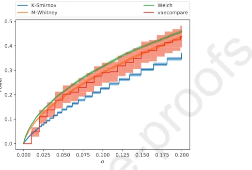
4.3. Evaluation (comparison with other methods)

Next, we apply our proposed hypothesis testing method (using the me- dian as the averaging function and 10 refits) to simulated datasets from a known data generating function and compare it with other well established two-

255

sample comparison methods: Mann-Whitney rank test[Mann47], Kolmogorov- Smirnov[Smirnov48] and Welch’s t-test[WELCH1947].

Given that such methods work only with univariate datasets, we choose the true distribution of the generating data to be a mixture of 3 equiprobable Gaussian distributions with means -2, 0 and 2 and standard deviation 1. For

260

testing the alternative hypothesis, one of the datasets had a 0.1 disturbance added (i.e., the dataset is generated from a mixture of 3 equiprobable Gaussian distributions with means -2.1, 0.1 and 2.1). Each dataset being compared is composed of n= 1000instances generated independently from the true distri- bution. Due to computational limitations, the power function was estimated

265

using 500 simulations for vaecompare, while we used 10000 simulations for the other tests.

Figure5shows the mean test power of each test with a confidence band of 2 times the standard error (i.e., an approximately 95% confidence). In order to make the visualization of the results easier, we also present a smoothed version

270

of this figure in Figure6with smoothing done by simple point interpolation⁷. The figures indicate that vaecompare had competitive performance when compared to the other methods.⁸ Additionally, it is the only method that can be used exploratory data analysis (on two-sample comparison) instead of just hypothesis testing and moreover, as shown in Section4.2, the test power could

275

potentially increase if an additional number of refits, which were set to be a small number because of the computational restrictions of the simulation study.

7Such smoothed version could also be obtained by increasing the number of permutations for each test, this has not been done due to computational constraints of such increase.

8Note in particular, that, contrary to the problems of classification and regression, is not possible to easily data split the dataset to choose the best hypothesis testing method before applying it the whole dataset (at least not without causing further problems such as bias multiple comparisons).

Figure 5: Comparison of vaecompare with other hypothesis testing methods. Our procedure shows good power.

Figure 6: Comparison of vaecompare with other hypothesis testing methods. Points outside of the grid are smoothed by interpolation. Our procedure shows good power.

5. Discussion and Conclusions

In this work, we proposed and applied a novel method of two sample distance measurement and hypothesis testing to simulated and real-world datasets. We

280

conclude that both two sample distance measurement and hypothesis testing were able to satisfactorily perform the intended tasks on the tested simulated and real world datasets.

The proposed methods could be used for various tasks in the machine learn- ing pipeline, including:

285

• Distribution shift detection and measurement: a dataset from a experi- ment done in one month (e.g.: opinions of customers on a product on a specific month) might diverge in distribution from a dataset collected in another month. With our method it is possible to measure and test this diverge.

290

• Dataset split: to address overfitting, the data is usually split into train, val- idation and/or test parts. To be able to develop robust models, these parts should be similar, but should also differ enough to ensure generalization.

With the proposed methods the dataset split can be done in a controlled manner, an important speed on state-of-the-art predictive methods (e.g.:

295

seeBreiman1996StackedR, Coscrato2020and references therein).

• Self-supervised clustering: based on the distance, by fine-tuning the thresh- old (cutpoint), binary or multi-class clustering could be performed.

• Anomaly detection: applying the proposed method to processes where anomaly may occur (e.g. malicious attack, malfunction, etc.). In this

300

case, the distance measurement can give a direct feedback of how much the actual behaviour differs from the normal one.

• To test the quality of data generated from GANs and similar approaches (e.g.: seebinary-two-sample).

Acknowledgments

305

Marco Inácio is grateful for the financial support of CAPES (this study was financed in part by the Coordenação de Aperfeiçoamento de Pessoal de Nível Su- perior - Brasil (CAPES) - Finance Code 001). Marco Inácio is also grateful for the financial support of the Erasmus Plus programme. Rafael Izbicki is grateful for the financial support of FAPESP (grants 2017/03363-8 and 2019/11321-9)

310

and CNPq (grant 306943/2017-4). Bálint Gyires-Tóth and Marco Inácio are grateful for the financial support of the BME-Artificial Intelligence FIKP grant of Ministry of Human Resources (BME FIKP-MI/SC). Moreover, Bálint Gyires- Tóth is also greateful for the financial support of Doctoral Research Scholarship of Ministry of Human Resources (ÚNKP-19-4-BME-189) in the scope of New

315

National Excellence Program, by János Bolyai Research Scholarship of the Hun- garian Academy of Sciences. The authors are also grateful for the suggestions given by Rafael Bassi Stern and by anonymous referees.

Appendix: Neural networks configuration, software and package We work with a dense neural network of 10 layers with 100 neurons on each

320

layer (totaling 195060 parameters), for both encoder and decoder networks, and the following additional specification:

• Optimizer: we work with the Adamax optimizer [adam-optim] with initial learning rate of 0.01 and decrease its learning rate by half if im- provement is seen on the validation loss for a considerable number of

325

epochs.

• Initialization: we used the initialization method proposed by [nn-initialization].

• Layer activation: we chose ELU [elu] as activation functions.

• Stop criterion: a 90%/10% split early stopping for small datasets and a higher split factor for larger datasets (increasing the proportion of train-

330

ing instances) and a patience of 50 epochs without improvement on the validation set.

• Normalization and number of hidden layers: batch normalization, as proposed by [batch-normalization], is used in this work in order to speed-up the training process.

335

• Dropout: here we also make use of dropout which as proposed by [dropout]

(with dropout rate of 0.5).

• Software: we have PyTorch[NEURIPS2019_9015] as framework of choice which works with automatic differentiation and the sstudy Python package[2004.14479] for organizing the simulation studies and compar-

340

isons. Moreover, the software implementation of this work is available at https://github.com/randommm/vaecompare.

Additionally, we present in Figures 3 and 4 the algorithm to evaluate the encoder and decoder neural networks, respectively.

Algorithm 3Algorithm to evaluate encoder network g(.) presented in Figure1 Input: x,

Output: µ,σ.

1: val = x

2: fori∈ {1,10}do

3: val = linear(val) (with output size 100).

4: val = ELU(val).

5: val = batch_norm(val)

6: val = dropout(val)

7: end for

8: µ= linear(val)

9: σ=exp{linear(val)}.

Algorithm 4Algorithm to evaluate decoder network h(.) presented in Figure1 Input: z, distribution

Output: (µ,σ) orp.

1: val = z

2: fori∈ {1,10}do

3: val = linear(val) (with output size 100).

4: val = ELU(val).

5: val = batch_norm(val)

6: val = dropout(val)

7: end for

8: if distribution is "gaussian" (i.e. continuous data)then

9: µ= linear(val)

10: σ =exp{linear(val)}.

11: else if distribution is "bernoulli"then

12: p= sigmoid{linear(val)}.

13: end if