Dynamic System Using Conjunctive Operator

Dynamic System Using Conjunctive Operator

József Dombi

Árpád tér 2, H-6720 Szeged, Hungary, email: dombi@inf.u-szeged.hu

József D. Dombi

Árpád tér 2, H-6720 Szeged, Hungary, email: dombijd@inf.u-szeged.hu

Abstract: We present a tool to describe and simulate dynami systems. We use positive and negative influences. Our starting point is aggregation. We build positive and negative effects with proper transformations of the sigmoid function and using the conjunctive operator. From the input we calculate the output effect with the help of the aggregation operator. This algorithm is comparable with the concept of fuzzy cognitive maps.

Keywords: dynamic system, pliant concept, dombi operator

1 Introduction

We usually face serious difficulties when we handle sophisticated dynamic systems. Developing a model requires effort and specialized knowledge. Usually a system involves complicated causal chains, which might be nonlinear. It should also be mentioned, that numerical data may be hard to get, they can be even uncertain. Using a classical dynamic system model can be hard computationally.

Fuzzy Cognitive Map (FCM) approach overcomes the above mentioned difficulties. FCM was proposed by Kosko [1][2][3] and is a hybrid method that lies in some sense between fuzzy systems and neural networks. Knowledge is represented in a symbolic manner using states, processes and events. All type of informations have numerical values. FCM allows us to perform qualitative simulations and experiment with a dynamic model. FCM has better properties than expert systems, since it is relatively easy to use them to represent structured knowledge and the inference can be computed by numeric matrix operation instead of applying rules. Our solution is similar to FCM. It is called Pliant Cognitive Map (PCM). It is based on a qualitative description of the influences, i.e. it is enough to know a rough description of the system. The main difference

between PCM and FCM is the replacement of matrix multiplication by fuzzy operators.

2 Short Description of FCM

In FCM the causal relationship is expressed by either positive or negative signs ordered by different weights. As we mentioned this will be replaced by unary operators in PCM.

Let {C1, . . . ,Cm} be concepts. Define a directed graph over the concepts. We assign a weight wij

∈

[0, 1] to the edge directed from concept Ci to concept Cj . The weight measures the influence of Ci on Cj . If the wij = 1/2 then wij is called neutral value. If wij = 0 then we say it is a maximum negative influence, if wij = 1 then we say it is a maximal positive influence or causality (In FCM wij

∈

[−1,0, 1]):

• wij > 1/2 indicates direct (positive) causality between concepts Ci and Cj. That is the increase (decrease) in the value of Ci leads to increase (decrease) on the value of Cj.

• wij < 1/2 indicates inverse(negative) causality between concepts Ci and Cj. That is the increase (decrease) in the value of Ci leads to decrease (increase) on the value of Cj.

• wij = 1/2 indicates Ci and Cj are neutral to each other.

In the pliant case wij depends on time (t), i. e.

( )

( ) _ij( ) w t w t n n

= × (1)

The activation level ai of concept Ci is calculated by an iteration process. In FCM (2)

where a_iⁿ is the new activation level of concept Ci at time t+1, a_i⁰ is the activation level of concept Ci at time t and f is the threshold function. FCM has the advantage that we obtain the new state vector by multiplying the previous state vector by the edge matrix W that shows the effect of the change in the activation level of one concept to another concept.

3 Basic Concept of PCM

In this paper we modify the concept of FCM. We use cognitive maps to represent knowledge and to model decision making, which was introduced by Axelrod. The cognitive map describes the whole system by a graph showing the cause effects along concepts. It is a directed graph with feedback, that describes the concepts of the world and the casual influences between the concepts. From logic point of view the causal concepts are unary operators of a continuous valued logic containing negation operators in the case of inhibition effects. The value of a node reflects the degree of the activity of the system at a particular time. Concept values are expressed on a normal [0, 1] range. Kosko used fuzzy values and matrix multiplication to calculate the next state of the systems.

We drop the concept of matrix multiplication. The matrix multiplication does not suit well in continuous logic (or fuzzy logic), where the truth value is 1 and the false is 0. General operators are more effective.

Logic and the cognitive map model correspond to each other in the PCM. It is easier to build up a PCM. After we identified the PCM with the real world, extracting the knowledge is easy. Combination of cognitive maps with logic helps us extracting knowledge more efficiently opposed to the use of rule based systems. The classical knowledge representation in expert systems is made through a decision tree. This form of knowledge presentation in most cases cannot model the dynamic behavior of the world. Instead of values, we use time dependent functions that are similar to impulse functions which represent positive and negative influences.

Values do not denote exact quantities, they denote the degree of activation. The inverse of normalization could express the values coming from the real world i.e.

using sigmoid function. In spite of Fuzzy Cognitive Maps we do not use thresholds to force the values between 0 and 1. The mapping is a variation of the fuzzification process in fuzzy logic, furthermore it always destroys our desire to get quantitative results. In pliant logic we map the real world into logic. These maps are continuously strict monotonously increasing functions, and so the inverse of these functions yields the data of the real world.

In the pliant concept we aggregate the influences instead of summing up the values. The result always remains between 0 and 1, so we can avoid normalization as an additional step. The aggregation in pliant logic is a general operation, which contains conjunctive operators and disjunctive operators as well. Depending on the parameter called neutral value of the aggregation operator we build logical operators (Dombi operators).

Using PCM (Pliant Cognitive Maps) we answer what if questions based on an initial scenario. Let a0 be the initial state vector. The new state is calculated

repeatedly with the aggregation operator until the system converges i. e.

.

We obtain the resulting equilibrium vector, which provides the answer to our what-if questions. The PCM can be used in all areas covered by FCM.

4 Components of PCM

4.1 Negation

The properties of negation are:

• defined on (0,1) and the values are also in (0,1)

• n(0) = 1

• n(1) = 0

• continuous

• strictly decreasing function

• involutive, n(n(x)) = x

•

n ( υ ) = υ

₀ or n(

υ

_*)=

υ

_*

The corresponding negation function in PCM is

(3)

(4)

4.2 Conjunction and Disjunction

Using an impulse function we can create positive and negative influences. Our task is to produce this function. The function is defined in time line and maps to [0, 1]. To construct this function we use a fuzzy operator and sigmoid function. It is important to consider that the fuzzy operator and sigmoid function fits well,

accordingly we use Dombi[5] operator. The associative function equation is the following:

)) ( ) ( ( )

,

(x y f ¹ f x f y

c = _c⁻ _c + _c

d ( x , y ) = f

_d⁻¹

( f

_d

( x ) + f

_d

( y ))

(5) We call c(x,y) and d(x,y) pliant system if

f

_c

( x ) + f

_d

( x ) = 1 .

The function of

Dombi operators are pliant systems and:

x x x f

x x

f

_{c c}

= +

= −

⁻

1 ) 1 ( 1 ,

)

(

¹ , ¹ ₁

1

1 ) 1 ( 1 ,

)

(

⁻ ₋

−

= +

⎟ ⎠

⎜ ⎞

⎝

= ⎛ −

x x x f

x x

f

_{d d} (6)

If we use Dombi operator in the conjunction and disjunction function we get the following equation:

( , ) 1

1 1

1 c x y

x y

x y

= + − + −

, ₁

1 1

( , ) 1

1 1

1 d x y

x y

x y

− −

= −

⎛⎛ − ⎞ ⎛ − ⎞ ⎞

⎜ ⎟

+⎜⎝⎜⎝ ⎟⎠ +⎜⎝ ⎟⎠ ⎟⎠

(7)

Using the Dombi operator we get the powered function in the following form:

1

( , ) 1

1 1

1 o x y

x y

x y

λ λ λ

=

⎛⎛ − ⎞ ⎛ − ⎞ ⎞

⎜ ⎟

+⎜⎝⎜⎝ ⎟⎠ +⎜⎝ ⎟⎠ ⎟⎠

(8)

If

λ

>0 then it is conjunction function, if

λ

<0then it is disjunction function.

If we pay attention to the general form of the weight we can generalize the formula. In this case we lose the associativity property, however we get other good properties, which are very useful (i.e. idempotency). Let u and v be the weights, with the following qualities: u+v=1, 0<=u,v<=1. With these restriction we get the generalized function:

1

( , ; , ) 1

1 1

1 o u x v y

x y

u v

x y

λ λ λ λ

=

⎛ ⎛ − ⎞ ⎛ − ⎞ ⎞

⎜ ⎟

+⎜⎝ ⎜⎝ ⎟⎠ + ⎜⎝ ⎟⎠ ⎟⎠

(9)

4.3 Aggregation

Beside the developed logical operators in fuzzy theory, a non logical operator also appears. The reason for this is the insufficiency of using either conjunctive or disjunction operators for real world situations.

The aggregation operator is axiomatically based and it has several good properties as:

• defined on (0,1) and the values are also in (0,1)

• associativity

• strictly monotonously increasing

• continuous on [0,1) interval

• a(0,0) = 0 and a(1,1) = 1

The rational form of an aggregation operator [4] is:

(10) Aggregation is connected to negation operators. The negation function and the aggregation operator are closely related. It can be easily seen that:

• n(a(x,y)) = a(n(x),n(y))

• a(x,n(x)) = v0

• a(x,v0) = x

These properties of the aggregation are natural:

• Aggregating positive values and negating is the same as aggregating negative values

• By aggregating a positive and its negated value we get the neutral values back

• Aggregating x with the neutral value we get back x.

We can model conjunctive and disjunctive operators with the aggregation operator. If v is close to 0 then the operation has a disjunctive characteristic and if v is close to 1 then the operation has a conjunctive characteristic. From this property it can be seen, that by using aggregation we have more possibilities than by using the sum function in FCM. By changing the neutral values at the nodes different operations can be carried out.

5 Components of PCM

The sigmoid function naturally maps the values to the (0,1) interval. Positive (negative) influences can be built with the help of

σ

_a^λ1,

σ

_b^λ2 and the conjunctive operator, where

λ

₁ >0,

λ

₂<0 and a < b.

Using weighted conjunction, it is worth to choose the following values

2 1

2

λ λ

λ

= +

u

,

2 1

1

λ λ

λ

= +

v

. So we get the generalized positive impulse function:

(11)

Figure 1

Asymmetrical positive influence on [0, 1]

If the influence is neutral, we represent it by 1/2 value. If there are no influences, then we continuously order 1/2 value to the system. If we want to model positive influences, we order a value, which is larger than 1/2, and maximal value is 1. The negative influence is the negation of the positive influence. To create these influences we use the following transformations:

(12)

(13)

Figure 2

Transformation of 2 Positive and 2 Negative influences

To simulate the system the only thing we have to do is to aggregate the influences.

The aggregation operator is a guarantee, that we use influences in the right manner. If we know the real process, then our task is to divide the function values into positive and negative influences. It is an optimalization problem. Starting the optimalization we need initial values. This is the critical point the success of optimalization. If we set it wrong, then the optimalization method finds only the local optimum, but the shape of the real process can help us. We can find the starting and the end points of the influences, even we can estimate the

λ

parameters. These initial values guarantee that the optimalization method with a high probability finds global optimum. This gives us a new method to analyze real process.

Figure 3

Aggregation of the influences

6 Construction of Dynamic Sytem

With the above mentioned procedure, it is easy to build PCM. The following steps should be carried out:

1 Collect the concepts.

2 Define the expectation values of the nodes (i.e. threshold values of the aggregations).

3 Build a cognitive map (i.e. draw a directed graph between the concepts).

4 Define the influences (i.e. are they positive or negative).

The iterative method:

i Use the proper function or give a timetable for the input nodes.

ii Calculate the positive and negative influences using step 4.

iii Aggregate the positive and negative influences, where the

υ

_∗ value is the previous value of Cj.

The system is now ready to make a simulation test. We developed a program in JAVA to test the system. First we study artificial situations. These situation show that the system is very flexible and is easy to adapt to various situations.

Simulation is based on directed graphs. The nodes are illustrated with squares.

Between the nodes there are edges. Instead of using arrows, we represent the direction of the edge by a filled circle. If the edge leads from the vertex v to vertex u, then we place the filled circle closer to u. (see Fig. 4). In Fig. 4 an example is given with two nodes and the direction between the nodes is from 2 to 1.

Figure 4 Graph representation

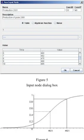
In Fig. 4 index 2 is input node and 1 is inner node. If node is an input node, then instead of giving the initial value we give the input data. There are three types to add new input data: using

• table, we can set input data by our self in every time period.

• Algebraic functions, (sin, cos, exp, sigmoid, etc.), calculate the selected function values.

• Generate Noise: we generate random numbers by normal distribution between 0.5 ,0 .5 (default: 0.1),

which is simulated noise.

See Fig. 5.

The input values are transformed into [0,1] with the sigmoid function:

f_sig 1

1 e ^{x x0 ,}

where

x

₀is the basic value (the expectation level), and

λ

is the sharpness of the function. It is reasonable to set

min max

4 x

x −

λ =

, because

λ

is the slope of the sigmoid function., where

x

_max,(x_min)is the largest (smallest) value.

Figure 5 Input node dialog box

Figure 6

The next step is to connect the nodes. To add a new edge, we give

• the index of the source node

• the index of the destination node

• the influence (positive or negative)

• the expectation value(

ν

).

7 Simulation Process

So we have the system. Now we can start the simulation. In one cycle the following calculation are made:

1 For all edges we calculate the influences.

i We find the source of the edge

ii We transform the source value by the intensity:

) (

) ( 1

1 1

1

value node

value f

_edge

− node

+ −

=

ν

ν

^,

where is the edge expectation value.

iii We calculate the edge influence with a conjunctive function. If

=1

λ

then the influence is positive If

λ

=−1 then the influence is negative. We use the conjunctive function, since in the real world the influences never reach extreme values, i.e.: 0 and 1.

2 Calculate the new value of the nodes.

i We collect the influences that lead to the node ii We transform the influences, and multiply all of them

f_inftr 1 f_{inf value}

i

f_{inf value}

i

iii We use the following function to get the actual value:

) (

) ( 1 1

1

inf )

(

value node

value f node

f

tr value

nodenew

= + −

,

which is an aggregation.

3 Set the actual value of input node.

In the future, for the real world applications we invent learning processes to find the best parameter. This leads to a nonlinear problem.

8 Results

Now we can run the dynamic system and check whether the developed PCM concept fulfills the basic properties.

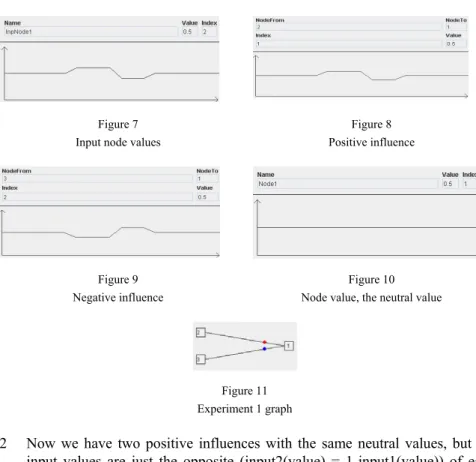
1 We have two input nodes with the same υ value. They always take the same values, but the influences are opposite, one is positive and the other is negative. These two input nodes have one common inner node. The result should be the neutral value (0.5). See Figs. 7, 8, 9, 10, 11.

Figure 7 Input node values

Figure 8 Positive influence

Figure 9 Negative influence

Figure 10 Node value, the neutral value

Figure 11 Experiment 1 graph

2 Now we have two positive influences with the same neutral values, but the input values are just the opposite (input2(value) = 1-input1(value)) of each other. The result should be also a neutral value. We can also check this by using sin(x) and cos

(

x+

π

/2

)

. See Figs. 12, 13, 14.

Figure 12 Positive influences of sin(x)

Figure 13

Positive influences of cos

(

x+

π

/2

)

Figure 14

The result of the aggregation of two positive influences

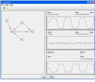
3 It is a small complex system with three inputs and two inner nodes. Two input nodes generate noises with different intensity; the third one is a periodical function. See Fig. 15.

Figure 15 Small complex system

Conclusions

We propose a new type of numerical calculus to model complex systems based on positive and negative influences. This concept is similar to FCM, but the functions and the aggregation procedures are quite different. It is based on acontinuous

valued logic and all the parameters have semantic meaning. We are working on a real world application and on an effective learning of the parameters of the system.

References

[1] Kosko B.: A dynamic system approach to machine intelligence, Neural networks and fuzzy Systems, 1992

[2] Kosko B., Dickerson J.: Fuzzy virtual worlds, AI Expert, 1994

[3] Kosko B.: Fuzzy Cognitive Maps, nt. Journal of Man Machine Studies, Vol. 24, 1986, pp. 65-75

[4] Dombi J.: Basic concept for a theory of evaluation: the aggregation operator, Europian Journal of Operations Research, Vol. 10, 1982, pp. 282- 293

[5] Dombi J.: A general class of fuzzy operators, the De Morgan class of fuzzy operators and fuzziness measures induced by fuzzy operators, Fuzzy Sets and Systems, Vol. 8, 1982, pp. 149-163