Single-shot extreme-ultraviolet wavefront measurements of high-order harmonics

Single-shot extreme-ultraviolet wavefront measurements of high-order harmonics

H

D

,

H

C

-A

,

C

G

,

E

K

,

F

C

,

J

L

,

J

P

,

H

W

,

B

M

,

E

M

,

D

A

,

K

V

,

C

L. A

,

G

D

,

P

J

,

A

L’H

,

S

M

,

P

R

,

P

Z

1Laboratoire d’Optique Appliquée, École Nationale Supérieure de Techniques Avancées, École Polytechnique, CNRS UMR7639, Chemin de la Hunière, 91761 Palaiseau Cedex, France

2Department of Physics, Lund University, P. O. Box 118, SE-22100 Lund, Sweden

3Imagine Optic, 18 Rue Charles de Gaulle, 91400 Orsay, France

4ELI-ALPS, ELI-HU Non-Profit Ltd., Dugonics ter 13, Szeged 6720, Hungary

*hugo.dacasa@fysik.lth.se

Abstract: We perform wavefront measurements of high-order harmonics using an extreme- ultraviolet (XUV) Hartmann sensor and study how their spatial properties vary with different generation parameters, such as pressure in the nonlinear medium, fundamental pulse energy and duration as well as beam size. In some conditions, excellent wavefront quality (up toλ/11) was obtained. The high throughput of the intense XUV beamline at the Lund Laser Centre allows us to perform single-shot measurements of both the full harmonic beam generated in argon and individual harmonics selected by multilayer mirrors. We theoretically analyze the relationship between the spatial properties of the fundamental and those of the generated high-order harmonics, thus gaining insight into the fundamental mechanisms involved in high-order harmonic generation (HHG).

© 2019 Optical Society of America under the terms of theOSA Open Access Publishing Agreement

1. Introduction

High-order harmonic generation (HHG) in gases [1, 2] is a highly nonlinear process which provides spatially and temporally coherent ultrashort pulses [3, 4] in the extreme ultraviolet (XUV) and X-ray domains [5–7]. HHG has applications in many research fields, such as nonlinear XUV optics [8], attosecond physics [9, 10], XUV spectroscopy [11], and plasma physics [12, 13].

Generating high-order harmonic beams with high spatial quality is of crucial importance for applications like imaging [14], holography [15], or as a seed of a plasma amplifier [16] or a free-electron laser [17]. Good spatial quality also allows for tighter focusing [18–21], leading to higher intensities, important for experiments involving nonlinear phenomena, such as two-photon ionization of gases [22, 23]. The study of harmonic wavefronts can lead to better knowledge of the physical process of HHG, and suggest new ways of optimizing the resulting XUV beams in terms of power and spatial quality.

One of the first experiments performed to study the wavefronts of high-order harmonics made use of the technique of point diffraction interferometry [24] with, however, limited precision in the wavefront measurements. Furthermore, only the defocus was characterized, without measuring other aberrations such as astigmatism or coma. Other similar techniques include lateral shearing interferometry [25] and slit diffraction, also called spectral wavefront optical reconstruction by diffraction (SWORD) [26, 27]. The latter involves measuring the radiation diffracted from a slit scanned in front of a spectrometer, thus measuring the wavefronts and intensity profiles along

#349968

Journal © 2019 https://doi.org/10.1364/OE.27.002656

Received 2 Nov 2018; revised 19 Dec 2018; accepted 19 Dec 2018; published 28 Jan 2019

one direction for all harmonic orders simultaneously. This method is well suited for sources where rotational symmetry can be assumed, which is not the case in the present work. Complete two-dimensional measurements of the wavefront can be achieved by rotating the measurement setup by 90^◦. In either case, this technique always requires many laser shots per measurement.

XUV Hartmann wavefront sensors (WFS), while lacking the spectral resolution found in SWORD, provide high accuracy and allow for the measurement of the two-dimensional wavefront and intensity profile of a light pulse simultaneously [28]. Previous measurements of the wavefronts of high-order harmonics with this method use multiple shots [29, 30], required for HHG with infrared (IR) lasers with pulse energies in the few mJ range, repetition rates of the order of kHz, and short focal lengths. Thousands of shots are typically needed to be accumulated in order to record usable wavefront and intensity maps, thus providing only averages and no information on shot-to-shot stability. Hartmann sensors have, however, the potential for single-shot acquisitions provided that the measured pulse carries enough energy.

In HHG, a spectrum of several odd-order harmonics of the fundamental is obtained, corre- sponding in the time domain to an attosecond pulse train (APT). Depending on the application, it is interesting to measure the wavefront of the APT or of the individual harmonic components. The latter measurements require separation or selection of the harmonics, e.g. with multilayer mirrors, or the use of spectrally-resolved techniques such as SWORD or the Hartmann sensor-based method developed in [31]. Full beam APT wavefront measurements are useful to optimize and characterize the focus of attosecond pulses [21].

In this paper, we report the results of an experiment carried out at the intense XUV beamline at the Lund Laser Centre, with the main goal of investigating how the harmonic wavefront relates to the spatial properties of the driving IR beam. Another goal was to study in detail how it varies depending on the generation parameters, such as pressure of the nonlinear medium, diameter of the fundamental beam, and its pulse energy and duration. This is, to the best of our knowledge, the first systematic study of the effects these parameters have on the wavefronts of APTs based on single-shot measurements. Such measurements were made possible by the high throughput of this beamline, and provide useful information about the shot-to-shot variations of the XUV wavefronts. Additionally, we used multilayer mirrors to measure how the spatial properties change with the harmonic order. The obtained data can thus give insight on the fundamental mechanisms involved in HHG. We then present a new theoretical model of the wavefront transfer from the fundamental pulse to the harmonics, as well as numerical simulations based on it to explain the data from the experiment. Lastly, we use a deformable mirror (DM) on the IR beampath to modify the wavefront of the driving beam, and we studied its influence on the harmonic wavefronts. We found that using it led to significant improvement of the spatial quality of the high-order harmonics as well as the conversion efficiency.

2. Experimental setup

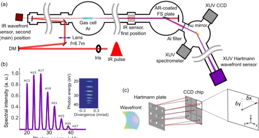
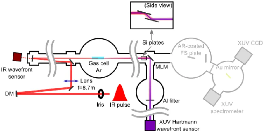
The setup used in this experiment is shown in Fig. 1(a). The Ti:Sapphire laser emits linearly polarized 40-fs pulses of 800-nm wavelength, at a repetition rate of 10 Hz. The high-order harmonics are generated in loose focusing geometry to optimize the conversion efficiency [32], by using a lens with a focal length of 8.7 m, and a 6-cm-long cylindrical gas cell filled with argon.

The IR beam, which has a 1/e²diameter of 35 mm, can be apertured by an iris placed before the lens. Between this iris and the lens there is a DM used at normal incidence. It contains 32 actuators which can modify the IR wavefront aberrations as well as its curvature. The DM was not used for the measurements reported in sections 3 and 4.

After the cell, the harmonic and IR beams propagate towards a fused silica plate, set at a grazing angle of 10^◦. The plate reflects XUV radiation (R=50%), but transmits most of the IR energy thanks to an anti-reflective coating. The beams then propagate through a 200-nm-thick aluminum filter, that blocks the remaining IR field, and towards a gold-coated flat mirror. The

mirror can be rotated in order to reflect the harmonic beam towards a spectrometer, the XUV Hartmann WFS, or a CCD camera to record its far-field intensity profile. The camera has been calibrated so that it can measure XUV energies as well. Figure 1(b) shows a typical harmonic spectrum generated in this setup.

Iris Lens f=8.7m IR wavefront

sensor, second (main) position

XUV Hartmann wavefront sensor XUV

spectrometer

XUV CCD

Gas cell Ar

AR-coated FS plate

Au mirror Al filter

IR pulse

Divergence (mrad) 0.2

0.4 0.6 0.8

-0.3 0.3

Photon energy (eV)

Photon energy (eV)

Mask XUV CCD

Spectral intensity (a. u.) Wavefront

Hartmann plate CCD chip (a)

(b)

(c)

δx δy

H17

H19

H21

H23 H25H27 H15

H13

1.0

20 30 40 20

30 40

IR sensor, first position

z y

x DM

Fig. 1. (a) Schematic drawing of the experimental setup for the measurement of single-shot high-order harmonic wavefronts. The Au mirror can be rotated to send the beam towards the XUV CCD camera or the spectrometer as well. (b) Typical harmonic spectrum generated in argon, including raw data showing the beam divergence. (c) Working principle of the XUV Hartmann wavefront sensor. The sensor contains an array of square subpupils and a CCD camera. An incoming wavefront is diffracted in each of them and propagated in a direction depending on the local slope. The resulting diffraction pattern is recorded on the CCD camera allowing for wavefront reconstruction. AR: Anti-reflective, FS: fused silica.

The working principle of the XUV Hartmann WFS is illustrated in Fig. 1(c). The WFS consists of a mask, also called a Hartmann plate, containing an array of holes, subsequently referred to as subpupils, placed before a CCD camera at a known distance. The direction of propagation of the beamlets upon diffraction by the subpupils is given by the local slope of the wavefront at the plane of the plate. The resulting diffraction patterns are recorded by the CCD camera, and their positions are then compared to reference positions, obtained via a previous calibration of the WFS, in order to reconstruct the wavefront [33].

The sensor used in this experiment was built and calibrated by the Laboratoire d’Optique Appliquée and Imagine Optic. The Hartmann plate contains 34x34 square subpupils of side 110 µm, separated by 387µm. They are rotated by 25^◦to prevent adjacent diffraction patterns from overlapping each other on the CCD camera [28], which is placed 211 mm after the Hartmann plate. Due to the low divergence of the harmonic beam, of the order of 0.2 mrad (see Fig. 1(b)), the sensor had to be placed as far as possible from the gas cell, about 9.5 m, in order to illuminate enough subpupils for an accurate wavefront reconstruction. The leakage from a flat mirror was used to monitor the wavefront of the driving IR beam with a Shack-Hartmann WFS [34].

It is important to note that the harmonic beam is reflected by two mirrors before being measured by the WFS. These optics introduce additional aberrations in the wavefront which might be significant, and must then be taken into account. To do so, we calibrated the optics by spatially filtering the high-order harmonic beam with a 100-µm pinhole placed in the beam path. This creates a beam with a known reference wavefront which is then reflected by the optics and measured by the WFS. Any aberrations present on this beam are thus solely caused by the optics.

3. Full-beam wavefronts

3.1. Single-shot high-order harmonic wavefronts

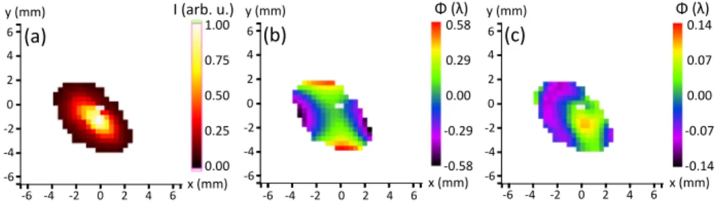
Throughout this experiment, we measured single-shot wavefronts for different values of the generation parameters. Figure 2 shows one such measurement, taken in the same generation conditions as the spectrum presented in Fig. 1(b). The measured quantity is the spatial phase variation perpendicular to the propagation axis. The obtained wavefront is compared to a perfect parabolic wavefront, and the difference is expressed in units of the central wavelength λ, where oneλcorresponds to a 2πradian phase variation. The quality of the wavefront is characterized by the root mean square (RMS) of the difference. In our case, the central wavelength isλ=λ_H19=42 nm, corresponding to the 19^thharmonic order. All RMS values are given as averages of five shots, together with the corresponding standard deviation, in order to show the shot-to-shot stability of the high-order harmonic beam.

As shown in Fig. 1(b), our HHG spectrum comprises mainly five harmonics. Using a theoretical model described in [42], in the conditions used in the present work, we find that the curvature difference between the harmonic wavefronts stays lower than 5% and close to the curvature of the full beam. In general, the full beam wavefront is expected to be an average of that of the individual harmonics.

Figures 2(a) and 2(b) show the intensity distribution and wavefront, respectively, of a single APT, after filtering out the defocus (i.e. the Zernike polynomial 2r²−1) and tilt components. In this case, the generated wavefront has an RMS value of(0.287±0.064)λ, close toλ/4, averaged over five separate single-shot measurements.

It is dominated by astigmatism at 0^◦, which is consistent with previous experiments carried out at high repetition rates [29]. The contribution of astigmatism to the wavefront can be numerically filtered out, resulting in Fig. 2(c). In this case, the RMS is only(0.062±0.006)λ, indicating the much lower contribution of all other aberrations, such as coma or spherical aberration.

x (mm) 1.00 0.75 0.50 0.25 0.00 I (arb. u.) y (mm)

(a)

-6 -4 -2 0 2 4 6 6

4 2 0 -2 -4 -6

y (mm)

(b)

Φ (λ) 0.58 0.29 0.00 -0.29 -0.58 -6 -4 -2 0 2 4 6

y (mm)

(c)

Φ (λ) 0.14 0.07 0.00 -0.07 -0.14 6

4 2 0 -2 -4 -6

-6 -4 -2 0 2 4 6 6

4 2 0 -2 -4

x (mm) -6 x (mm)

Fig. 2. Typical single-shot intensity distribution (a) and wavefront (b) of the harmonic beam, along with the resulting wavefront after numerically ruling out astigmatism (c).

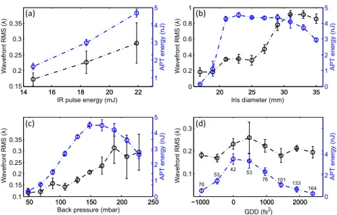
The main results obtained during the experiment are summarized in Fig. 3, where the harmonic wavefront RMS values are plotted with the energies of the APTs, measured with the calibrated CCD camera, when varying the IR pulse energy, the aperture diameter, the argon pressure, and the IR pulse duration (and with it the IR intensity). The latter is modified by introducing group delay dispersion (GDD) to the pulse with the compressor of the Ti:Sapphire laser chain. In each set of measurements, one parameter was varied, while the other ones were kept constant. All data points represent the average of five consecutive single-shot measurements, and the error bars represent the standard deviation.

The wavefront RMS was observed to vary significantly as a function of the generation conditions, even becoming as low asλ/10 or as high asλin some cases. It is also interesting to note that high APT energies are often paired with larger wavefront aberrations, so that a compromise must be made between having higher energies or better wavefronts. In all cases,

14 16 18 20 22 0.15

0.2 0.25 0.3 0.35

IR pulse energy (mJ)

14 16 18 20 22

1 2 3 4 5

−1000 0 1000 2000

0.1 0.2 0.3

53 42

76 133

53

76 101

164

GDD (fs²)

−1000 0 1000 2000 0

2 4

20 25 30 35

0 0.2 0.4 0.6 0.8 1

Iris diameter (mm)

20 25 30 35 0

1 2 3 4 5

50 100 150 200 250

0.1 0.15 0.2 0.25 0.3 0.35

50 100 150 200 2500

1 2 3 4 5

Back pressure (mbar)

APT energy (nJ)

APT energy (nJ)APT energy (nJ) APT energy (nJ)

(a) (b)

(c) (d)

Wavefront RMS (λ)Wavefront RMS (λ) Wavefront RMS (λ)Wavefront RMS (λ)

Fig. 3. Main data obtained in the experiment, representing the average wavefront RMS (black) of a single APT as well as its average energy (blue) as a function of (a) IR pulse energy, (b) iris diameter, (c) argon back pressure, and (d) GDD. The latter includes the calculated FWHM (full width at half maximum) duration of the IR pulses for each case, in fs, next to each data point.

however, the harmonic wavefronts were dominated by astigmatism, which may be corrected with appropriate focusing optics [21, 35, 36]. Additionally, the relative standard deviation for the wavefront RMS takes values between 15% and 20% in most cases, thus revealing a relatively good source stability, except for the most extreme cases such as those where the pressure was too high, or the iris was fully open.

The astigmatism always has similar directions, with only slight variations. We investigated the possibility that this direction is defined by the polarization of the IR beam by measuring harmonic wavefronts with three different IR polarization angles: vertical, horizontal, and at 45^◦. The direction of astigmatism, as well as the wavefront itself, remained constant, showing that the IR polarization has barely any influence on it or none at all. The calibration wavefront measured prior to the experiment has an RMS of(0.022±0.005)λ, around 10 times smaller than the full wavefront, indicating that the optics do not introduce any significant aberrations.

3.2. Relation between the IR and harmonic wavefronts

Being a secondary source of radiation, the spatial properties of harmonic radiation are expected to be influenced by those of the driving pulse. For this reason, the IR wavefront was measured prior to the experiment, by placing the IR Shack-Hartmann WFS 1.5 m after the gas cell (see Fig. 1).

This step was carried out at atmospheric pressure and without argon in the gas cell. Several neutral-density filters were placed before the focus to protect the sensor and to avoid nonlinear effects in air. A single-shot IR wavefront is shown in Fig. 4, obtained with typical beamline conditions. After these measurements, the sensor was placed behind a mirror to monitor the IR wavefront during generation through a leak in a mirror. Both positions of the IR sensor are equivalent in terms of distance to the focusing lens.

The IR beam is slightly elliptical, and the measured wavefront has an average RMS value of(0.095±0.003)λ_IR, better thanλ_IR/10. Astigmatism, which largely dominates every XUV wavefront measured throughout the experiment, is much less significant in the driving beam.

1.00

0.75

0.50

0.25

0.00

I (arb. u.) Φ (λIR)

x (mm) x (mm)

y (mm) y (mm)

0.27

0.12

0.00

-0.12

-0.27

-2.5 -1.5 -0.5 0 0.5 1.5 2.5 3

2 1 0 -1 -2 -3

-2.5 -1.5 -0.5 0 0.5 1.5 2.5 3

2 1 0 -1 -2 -3

(b) (a)

Fig. 4. Intensity distribution (a) and wavefront (b) of the direct IR beam in typical working conditions (λ_IR=800nm).

Additionally, the IR wavefront was observed to be constant throughout the experiment.

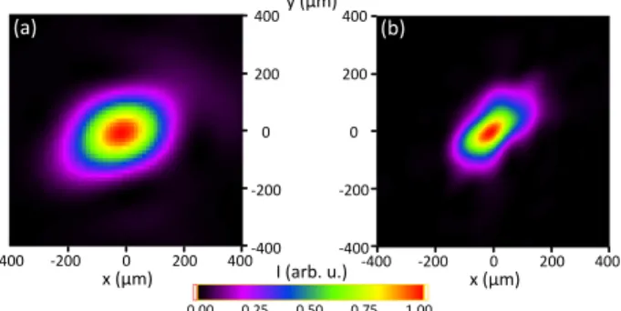
The IR focal spot in the gas cell reconstructed via back propagation of the measured far-field wavefront can be seen in Fig. 5(a). It has a slightly elliptical shape as well, and the average FWHM size was 239±1µm along the major axis and 178±1µm along the minor axis. Figure 5(b) presents the calculated harmonic source shape, obtained through back propagation of the measured spatial profile for typical generation conditions (see Fig. 2). Its average FWHM size was 211±5µm and 104±3µm along both axes. The size of the harmonic source was observed to vary depending on the generation conditions used, being smaller than the IR focal spot. This, in turn, is most likely caused by the nonlinearity of the HHG process, since the outer parts of the IR focus are not intense enough to efficiently generate XUV radiation.

x (μm)

-400 -200 0 200 400

(a)

x (μm)

-400 -200 0 200 400 400

200

0

-200

-400

(b)

0.00 0.25 0.50 0.75 1.00 400

200

0

-200

-400 y (μm)

I (arb. u.)

Fig. 5. Side by side comparison between the reconstructed infrared focus (a) and high-order harmonic source (b). Both images represent typical generation conditions.

4. Wavefronts of single harmonic orders

Different harmonic orders have been found to contain differences in their wavefronts [27]. For this reason, we used three dielectric multilayer mirrors, with peak reflectivities at different wavelengths, in order to isolate single harmonic orders in different parts of the spectrum and compare their wavefronts to each other and to that of the full beam. The optics were placed before the silica plate and the XUV Hartmann WFS was moved to a new position, as shown in Fig. 6. Since the silica plate is no longer used to filter the IR beam, two flat silicon mirrors at

Brewster’s angle are placed instead shortly before the mirrors. The multilayer mirrors consist of alternating layers of Al/Mo/SiC on fused silica substrates. They are all made for optimal use at 45^◦incidence, providing reflectivities around 35% for the wavelengths 41.4 nm (H19), 35 nm (H23) and 23.9 nm (H33). A 200-nm-thick aluminum filter is placed before the WFS. A calibration procedure such as the one described in section 2 was performed with each mirror, in order to rule out any aberrations they might introduce on the beam upon reflection [37].

Iris IR wavefront

sensor

XUV spectrometer

XUV CCD

Gas cell Ar

AR-coated FS plate

Au mirror

IR pulse

XUV Hartmann wavefront sensor MLM

(Side view)

Al filter DM

Lens f=8.7m

Si plates

Fig. 6. Experimental setup for the measurement of single harmonic orders with the use of multilayer mirrors, showing the new placement of the XUV WFS. Inset shows a side view of the silicon plates used to attenuate the IR beam. MLM: multilayer mirror.

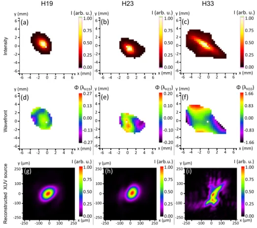
Although only one harmonic order was reflected by each mirror, the APTs had enough energy to allow for single-shot wavefront acquisitions, mostly due to the higher reflectivities of the involved optics, as well as the beam being smaller on the sensor due to the shorter distance to the cell, close to 7 m. As was done previously, five single-shot measurements were taken and averaged, to account for instabilities. Harmonics 19 and 23 were generated with very similar conditions. However, in order to observe a sufficient intensity of harmonic 33, the pressure and the aperture diameter had to be significantly increased. The XUV intensity profiles obtained with the three mirrors are presented in Figs. 7(a)-7(c). In general, the beam profiles are very similar for single harmonics and for the full beam shown above, except for the 33^rdorder, which is more elongated. This shape was also observed for the full beam at high pressures, which were required in order to generate this order efficiently.

The obtained wavefronts are presented in Figs. 7(d)-7(f), each represented in terms of its corresponding wavelength (denoted asλ_H19,λ_H23, andλ_H33). The aberrations introduced by the mirrors were calibrated and subtracted from these measurements. It can be seen that the 19^thorder presents no astigmatism, in contrast with the full beam, where astigmatism at 0^◦was always present. Slight astigmatism appears in the 23^rdorder, but it is still very low compared to the full beam. The 33^rdorder, on the other hand, is completely dominated by astigmatism at 0^◦. In particular, its angle of astigmatism is, on average, 8.0^◦, very close to the typical values observed in the full beam.

The average RMS values corresponding to the three orders were 0.062λ_H19=λ_H19/16, 0.084λ_H23=λ_H23/12, and 0.715λ_H33=λ_H33/1.3. In terms of units of length, these RMS values are 2.57 nm, 2.94 nm, and 17.09 nm, respectively. The relative standard deviation is close to 10% in all cases. In comparison, the full-beam wavefronts seen in Fig. 3 present values typically aroundλ_H19/4 andλ_H19/3 for conditions similar to those used for harmonics 19 and 23, which are observed to have much better wavefronts when isolated. Harmonic 33 is not generally observed in the setup, so the generation conditions were different from the other two orders. In particular,

x (mm) 1.00 0.75 0.50 0.25 0.00 I (arb. u.) y (mm)

(a)

-6 -4 -2 0 2 4 6 6

4 2 0 -2 -4

-6 x (mm)

y (mm)

(b)

I (arb. u.) 1.00 0.75 0.50 0.25

0.00

-6 -4 -2 0 2 4 6 x (mm)

y (mm)

(c)

I (arb. u.) 1.00 0.75 0.50 0.25 0.00 6

4 2 0 -2 -4 -6

-6 -4 -2 0 2 4 6 6

4 2 0 -2 -4 -6

x (mm) Φ (λH19) y (mm)

(d)

-6 -4 -2 0 2 4 6 x (mm)

y (mm)

(e)

Φ (λ_H23)

-6 -4 -2 0 2 4 6 x (mm)

y (mm)

(f)

Φ (λ_H33)

-6 -4 -2 0 2 4 6 4

6

2 0 -2 -4 -6

6 4 2 0 -2 -4 -6 6

4 2 0 -2 -4 -6 0.27 0.13 0.00 -0.13 -0.27

0.20 0.10 0.00 -0.10 -0.20

1.66 0.83 0.00 -0.83 -1.66

1.00 0.75 0.50 0.25 x (μm) 0.00

1.00 0.75 0.50 0.25 0.00 I (arb. u.) y (μm)

250 (g)

100 0 -100

-250

-250 -100 0 100 250 x (μm)

1.00 0.75 0.50 0.25 0.00 I (arb.u.) y (μm)

250 (h)

100 0 -100

-250

-250 -100 0 100 250 x (μm)

I (arb. u.) y (μm)

250 (i)

100 0 -100

-250

-250 -100 0 100 250

H19 H23 H33

IntensityWavefrontReconstructed XUV source

Fig. 7. Single-shot high-order harmonic intensity distributions (a-c), wavefronts (d-f), and reconstructed harmonic sources (g-i) for the 19^th, 23^rd, and 33^rdharmonic orders. Note that the wavefronts are expressed in terms of each order’s particular wavelength.

the pressure and IR pulse energies had to be increased, leading to distortions of the IR pulse in the medium via nonlinear effects [38], which may account for the more aberrated wavefront found in this harmonic order.

Lastly, the harmonic sources for each harmonic order, obtained via back propagation, are also presented in Figs. 7(g)-7(i). As expected from the measured wavefronts, the calculated sources for the 19^thand 23^rdorders are regular and slightly elliptical, similar to the best cases measured for the full harmonic beam, while it is slightly larger and highly distorted for the 33^rd. This order has, however, much lower intensity than the other two in typical working conditions, so it will not provide a large contribution to the shape of the full beam.

5. Theoretical interpretation

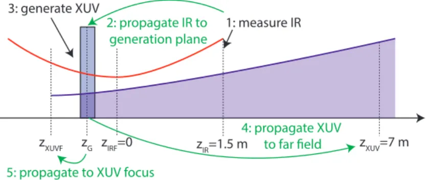
In order to better understand the spatial properties of high-order harmonics, we develop a simple model based on propagation by means of diffraction integrals and on a semi-classical description of the HHG process, neglecting propagation effects. The fundamental field evaluated in a certain planez_IR(see Fig. 8) can be written as a product of an amplitude and a phase term, as

E(x,y,z_IR) ∝ |E(x,y,z_IR)|exp(−iφ(x,y,z_IR)). (1) This field is then propagated to the generation position by calculating [39]

E(x,y,z_G)=FT⁻¹

E(k˜ _x,k_y,z_IR)exp

−i(z_G−z_IR) q

k²−k²_x−k_y² , (2) where ˜E_q(k_x,k_y,z_IR)is the spatial Fourier transform of the IR fieldE(x,y,z_IR).z_Gwas chosen to be -80 mm for H19 and H23 in the simulations presented below, and -130 mm for H33, in order to be consistent with the experimental measurements shown above.

1: measure IR 2: propagate IR to

generation plane 3: generate XUV

4: propagate XUV to far field

z_IR=1.5 m z_XUV=7 m z_G

z_XUVF z_IRF=0 5: propagate to XUV focus

Fig. 8. Principle of the simulations. The IR field is obtained from the experimental wavefronts and intensity maps recorded at positionz_IR. It is back propagated to the position z_G, where the harmonics are generated. The harmonic field is then propagated to the position z_XUV, where it is analyzed. Finally it can also be back propagated to its focusz_XUVF.

The generatedq^thharmonic field is approximated by

E_q(x,y,z_G) ∝ |E(x,y,z_G)|^pexp[−iqφ(x,y,z_G) −iφ_d(x,y,z_G)]. (3) The amplitude is assumed to vary slowly with the amplitude of the fundamental field, with a powerptypically of the order of 4 [40]. The phase of the harmonic field is the sum ofqtimes the phaseφ(x,y,z_G)of the IR field and the dipole phaseφ_d(x,y,z_G)originating from the generation process. Note that this simple model does not take into account propagation in the nonlinear medium or phase-matching effects. Considering only the short trajectory of the electron in the continuum, assumed to be classical, and neglecting spatially-independent terms, this phase can be approximated as [41, 42]

φ_d(x,y,z_G)=γ_s(q−q_p)²ω²

I(x,y,z_G) , (4)

whereγ_s =1.030×10⁻¹⁸s²Wcm⁻² for 800 nm wavelength andI(x,y,z_G)is the IR intensity.

The intensity is chosen to be 3×10¹⁴W/cm²for H19 and H23, and 4×10¹⁴W/cm²for H33, in order to replicate the experimental conditions. The quantityq_pis defined asI_p/~ω, whereI_pis the ionization potential andωis the IR frequency. The harmonic field is then propagated to a plane where it is spatially characterized (z_XUV) as in Eq. (2). It can also be back propagated to its focus (z_XUVF).

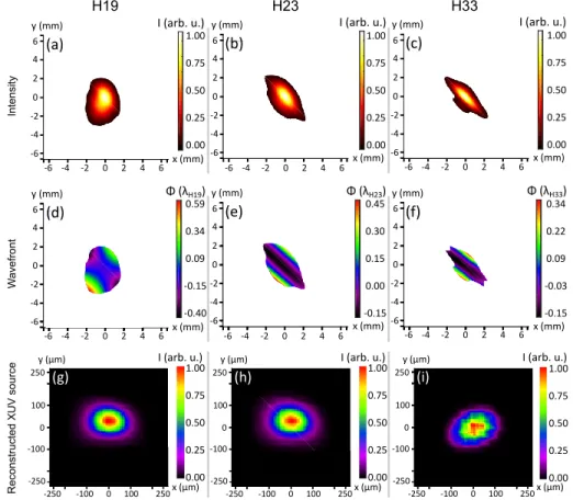
Figure 9 presents calculations of the 19^th, 23^rdand 33^rdharmonic fields using the measured IR field presented in Fig. 4. These simulated results can be compared with the experimental results in Fig. 7. In each case, we present the far field profile calculated atz=z_XUV=7 m, the wavefront and the reconstructed XUV source, calculated via back propagation. Experiments and simulations agree reasonably well for the far field intensity profiles. The beams were quite astigmatic around the XUV focal region in the simulations. The presented results are those obtained at approximately the medial focus. Finally, the XUV wavefronts are found to be

x (mm) 1.00 0.75 0.50 0.25 0.00 I (arb. u.) y (mm)

(a)

-6 -4 -2 0 2 4 6 6

4 2 0 -2 -4

-6 x (mm)

y (mm)

(b)

I (arb. u.) 1.00 0.75 0.50 0.25 0.00

-6 -4 -2 0 2 4 6 x (mm)

y (mm)

(c)

I (arb. u.) 1.00 0.75 0.50 0.25 0.00 6

4 2 0 -2 -4 -6

-6 -4 -2 0 2 4 6 6

4 2 0 -2 -4

H19 H23 -6 H33

x (mm) Φ (λH19) y (mm)

(d)

-6 -4 -2 0 2 4 6 x (mm)

y (mm)

(e)

Φ (λ_H23)

-6 -4 -2 0 2 4 6 x (mm)

y (mm)

(f)

Φ (λ_H33)

-6 -4 -2 0 2 4 6 4

6

2 0 -2 -4 -6

6 4 2 0 -2 -4 -6 6

4 2 0 -2 -4

-6 H33

H19 H23

0.59 0.34 0.09 -0.15 -0.40

0.45 0.30 0.15 0.00 -0.15

0.34 0.22 0.09 -0.03 -0.15

x (μm) I (arb. u.) y (μm)

250 (g)

100 0 -100

-250

-250 -100 0 100 250 x (μm)

I (arb. u.) y (μm)

250 (h)

100 0 -100

-250

-250 -100 0 100 250 x (μm)

I (arb. u.) y (μm)

250 (i)

100 0 -100

-250

-250 -100 0 100 250

H19 H23 H33

1.00 0.75 0.50 0.25 0.00

1.00 0.75 0.50 0.25 0.00

1.00 0.75 0.50 0.25 0.00

IntensityWavefrontReconstructed XUV source

H19 H23 H33

Fig. 9. Simulations of high-order harmonic intensity distributions (a-c), wavefronts (d-f), and reconstructed harmonic sources (g-i) for the 19^th, 23^rd, and 33^rdharmonic orders.

dominated by astigmatism, as in the experiment. The simulations reproduce qualitatively the measured wavefront.

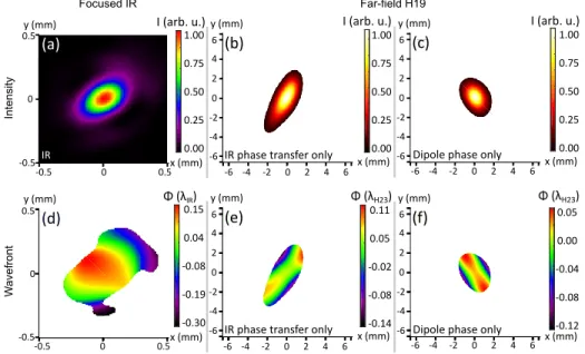
In Fig. 10, we show the respective influence of the IR phase aberrations which are transferred to the XUV and the effect of the dipole phase, which depends on the elliptical intensity profile of the IR, on the spatial properties of the 19^thorder. Comparing the wavefronts plotted in Figs. 10(e) and 7(d), we can conclude that the wavefront of the 19^thharmonic, which exhibits astigmatism at'45^◦, is mostly influenced by the IR phase. However, the harmonic intensity profile (see Fig. 9(a)) cannot be reproduced by considering only the IR phase transfer, and shows a strong influence of the dipole phase. In conclusion, both effects must be taken into account in order to understand the spatial properties of the generated harmonics, since they have a similar order of magnitude. Note that the interplay between IR phase transfer and dipole phase strongly depends on the generation conditions.

6. Using IR adaptive optics to improve the XUV wavefronts

Having demonstrated that the spatial properties of the high-order harmonics are strongly influenced by the wavefront and focusing of the driving pulses, it should then be possible to improve them by modifying the IR focus by means of adaptive optics. In this study, we analyzed how the spatial properties of the high-order harmonic beam, as well as the conversion efficiency, are modified with the use of the IR DM.

DMs have been used in the past to modify the wavefront of the driving beam for HHG in

x (mm) 1.00 0.75 0.50 0.25 0.00 I (arb. u.) y (mm)

(a)

-0.5 0 0.5 0.5

0

-0.5 x (mm)

y (mm)

(b)

I (arb. u.) 1.00 0.75 0.50 0.25

0.00 -6 -4 -2 0 2 4 6

x (mm) y (mm)

(c)

I (arb. u.) 1.00 0.75 0.50 0.25 0.00 6

4 2 0 -2 -4 -6

-6 -4 -2 0 2 4 6 6

4 2 0 -2 -4

IR IR-phase transfer only -6 Dipole phase only

Φ (λIR) y (mm)

(d)

x (mm) y (mm)

(e)

Φ (λH23)

-6 -4 -2 0 2 4 6 x (mm)

y (mm)

(f)

Φ (λ_H23)

-6 -4 -2 0 2 4 6 6

4 2 0 -2 -4 -6 6

4 2 0 -2 -4

-6 Dipole phase only

IR IR-phase transfer only

0.15 0.04 -0.08 -0.19 -0.30

0.11 0.05 -0.02 -0.08

-0.14 -0.5 0 0.5

0.5

0

-0.5

0.05 0.00 -0.04 -0.08 -0.12 x (mm)

0

IR phase transfer only

IR phase transfer only

Dipole phase only

Dipole phase only

Focused IR Far-field H19

IntensityWavefront

Fig. 10. Simulations of intensity distributions (a-c) and wavefronts (d-f) for the focused IR beam and far-field 19^thharmonic with the IR-phase transfer only and with dipole phase only.

setups with high repetition rates. This has been done to modify the astigmatism in the harmonic wavefront [29], and also to improve phase matching and thus the energy in the resulting APTs [43].

In the present work, we investigate the influence of the IR wavefront on the spatial properties of single high-order harmonic APTs, including all generated harmonic orders.

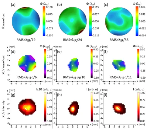
We simultaneously measured IR and harmonic wavefronts for different DM configurations, while all other previously mentioned generation parameters were kept unchanged. Figure 11 presents several measurements of the IR wavefront and the wavefront of the full harmonic beam, taken while modifying the DM in order to improve the latter. Each wavefront is normalized to its corresponding wavelength, with the RMS values included in the figure. The harmonic spectrum did not change significantly when varying the settings on the DM (see Fig. 1(b)).

Each column of Fig. 11 shows the IR and harmonic wavefronts, as well as the harmonic intensity distribution for one of the three cases presented. The first IR wavefront, seen in Fig. 11(a), has larger IR astigmatism than the rest. The resulting harmonic wavefront presents large astigmatism as well, but at 45^◦. The beam is also larger and has low energy. Figure 11(b) presents an intermediate case, where the DM configuration improves the IR wavefront and thus both the conversion efficiency and the harmonic wavefront. The resulting harmonic beam is smaller and less elliptical than observed in Figs. 2 and 7, as well as three times more energetic.

However, consistently with previous measurements, the harmonic wavefront is mainly astigmatic at 0^◦, whereas the IR wavefront presents more astigmatism at 45^◦. In the final configuration, shown in Fig. 11(c), the IR wavefront presents less aberration than in both 11(a) and 11(b).

However, this improvement does not significantly change the harmonic wavefront, which is only slightly better, having an RMS ofλ/11. The energy was not further increased from the previous measurement. In summary, by tweaking the DM to improve the IR wavefront, we were able to reduce the average XUV wavefront aberrations fromλ/4 toλ/11, as well as to increase the energy of the APTs by a factor of 3.

These results again show the importance of the IR beam’s spatial properties on the HHG process, since it affects not only the high-order harmonic beam wavefront, but also its shape and size, as well as the conversion efficiency. The experimental results clearly show that the

x (mm) Φ(λH19) y (mm)

(d)

-6 -4 -2 0 2 4 6 x (mm)

y (mm)

(e)

-6 -4 -2 0 2 4 6 x (mm)

y (mm)

(f) ^0.50

0.25 0.00 -0.25 -0.50 -6 -4 -2 0 2 4 6 0.50

0.25 0.00 -0.25 -0.50 0.50

0.25 0.00 -0.25 -0.50 4

6

2 0 -2 -4 -6

6 4 2 0 -2 -4 -6 6

4 2 0 -2 -4 -6

Φ(λH19) Φ(λH19) 0.064 0.032 0.000 -0.032 -0.064 Φ(λIR) 0.115

0.057 0.000 -0.057 -0.115 Φ(λIR) 0.150

0.075 0.000 -0.075 -0.150

Φ(λIR) (b) (c)

(a)

x (mm) 1.00 0.75 0.50 0.25 0.00 y (mm)

(g)

-6 -4 -2 0 2 4 6 6

4 2 0 -2 -4 -6

y (mm)

(h)

-6 -4 -2 0 2 4 6 x (mm)

y (mm)

(i) ^1.00

0.75 0.50 0.25 0.00 6

4 2 0 -2 -4 -6

-6 -4 -2 0 2 4 6 6

4 2 0 -2 -4 -6 1.00 0.75 0.50 0.25 0.00 x (mm)

RMS=λIR/19 RMS=λIR/24 RMS=λIR/53

RMS=λH19/6 RMS=λH19/10 RMS=λH19/11

Ix10 (arb. u) I (arb. u) I (arb. u)

IR wavefrontXUV wavefrontXUV intensity

Fig. 11. Direct comparison between the IR wavefronts measured with three different DM configurations (a-c) and the corresponding full-spectrum single-shot XUV wavefronts (d-f) and far-field intensity distributions for each case (g-i). The RMS values are included under each wavefront. Note that the intensity scale is different in (g) to make the beam more visible due to its lower energy.

XUV wavefront results from more than a just a direct transfer from the IR to the XUV, which is confirmed by the model presented above. The IR wavefront, however, is especially important due to how it affects its focusing. The use of the DM provided significant wavefront improvement with respect to the values typically found in previous measurements performed without it. The control it provides on the XUV wavefront is complex, since changing the IR wavefront modifies the intensity distribution at focus and thus the dipole phase during HHG (see previous section).

Nonetheless, using an IR DM provides a cheaper alternative to the use of less accessible DMs for the XUV domain [44].

7. Conclusions

The XUV Hartmann sensor provides a versatile tool for spatial metrology of pulsed XUV beams.

The single-shot harmonic wavefronts measured in this experiment had typical RMS values of the order ofλ/4. The high XUV energies obtained in this beamline allowed us to take single-shot high-order harmonic wavefront measurements, in turn providing information on the shot-to-shot wavefront stability. The relative standard deviation of the wavefront RMS takes values between 15% and 20% in most cases, thus revealing a relatively good source stability, except for the most extreme cases such as those with the highest pressures, or where the iris was fully open. It is also interesting to note that high XUV energies are often paired with larger wavefront aberrations.

The results of our single-shot wavefront measurements are similar to previously published

studies involving multishot measurements in beamlines with high repetition rates, in that the harmonic wavefront always presents a very prominent astigmatism, which was not observed in the IR beam. The fact that astigmatism is also observed in other high-order harmonic beamlines can be attributed to the difficulty in focusing the IR beam in a perfectly symmetrical manner.

The observed predominant direction of astigmatism, around 0^◦, might be due to the optics used to handle the IR beam. These include in particular a compressor at the end of the amplification chain, which has a similar geometry in most Ti:Sapphire laser systems and might introduce small aberrations that cause the focal spot to deviate from a perfect Gaussian profile. Other aberrations such as coma or spherical aberration are much less significant. In fact, if the astigmatism is corrected with appropriate focusing optics, RMS values lower thanλ/10 can be obtained, even diffraction-limited beams in some of the cases reported here before the use of the DM. It was found, however, that the best wavefronts are generally obtained at the cost of low harmonic energies. During this experiment, we also confirmed that the direction of polarization of the IR pulse has no influence on the harmonic wavefront. Additionally, the study of single harmonic orders by means of multilayer mirrors suggests that not all orders carry the same amount of astigmatism.

The experimental data indicate that the full spatial profile (amplitude and phase) of the IR affects the harmonics, rather than just its wavefront. We thus propose a theoretical model which describes the transfer of the spatial profile from the IR to the harmonics through two effects, the direct transfer from IR wavefront to XUV wavefront by frequency upconversion and the transfer from the IR intensity profile to the XUV wavefront through the dipole phase. The curvature induced by the dipole phase is generally comparable in magnitude to that due to the IR beam curvature, so it must be taken into account as well. It must be noted that the model does not account for phase matching effects or propagation of the IR pulse in the gas, so its results are not perfectly accurate at this stage. The simulations presented here show a satisfactory agreement with the experimental data when using typical generation conditions.

In conclusion, while the generation parameters affect the harmonic wavefront RMS, the shape of the IR focus was found to have a larger impact on the spatial properties of the XUV beam. We demonstrate that they can be improved to a large extent by using IR adaptive optics to modify the IR wavefront, and thus its focus. This also had a significant effect on the APT energy, increasing it by a factor of up to three compared to previous measurements without the DM. Being able to tailor the spatial properties of the harmonics with this method provides a useful alternative to the use of a more expensive DM for the XUV domain, which would also provide lower reflectivity.

Furthermore, a computerized closed-loop program could be implemented in the beamline, which would use data from the XUV sensor to find the DM configuration which provides the best harmonic wavefront, the highest energy, or the most circular beam shape.

Future steps involve improving the theoretical model as well as performing further experiments to learn more about the transfer of spatial properties in order to improve the quality of the generated XUV beams, as well as to compare the experimental results with the simulations. This, in turn, will lead to better focusing and thus higher XUV intensities.

Funding

Svenska Forskningsrådet Formas; Stiftelsen för Strategisk Forskning; Knutoch Alice Wallen- bergs Stiftelse; H2020 European Research Council (339253 PALP); LASERLAB-EUROPE (LLC002276); European Cooperation in Science and Technology (MP1203 and CM1204);

Horizon 2020 Framework Programme (665207); H2020 Marie Skłodowska-Curie (641789 MEDEA); European Regional Development Fund.

References

1. A. McPherson, G. Gibson, H. Jara, U. Johann, T. S. Luk, I. A. McIntyre, K. Boyer, and C. K. Rhodes, “Studies of multiphoton production of vacuum-ultraviolet radiation in the rare gases," JOSA B4(4), 595–601 (1987).

2. M. Ferray, A. L’Huillier, X. F. Li, L. A. Lompré, G. Mainfrays, and C. Manus, “Multiple-harmonic conversion of 1064 nm radiation in rare gases,” J. Phys. B21(3), L31–L35 (1988).

3. R. A. Bartels, A. Paul, H. Green, H. C. Kapteyn, M. M. Murnane, S. Backus, I. P. Christov, Y. Liu, D. Attwood, C.

Jacobsen, “Generation of spatially coherent light at extreme ultraviolet wavelengths,” Science297(5580), 376–378 (2002).

4. C. Lyngå, M. B. Gaarde, C. Delfin, M. Bellini, T. W. Hänsch, A. L’Huillier, and C.-G. Wahlström, “Temporal coherence of high-order harmonics,” Phys. Rev. A60(6), 4823 (1999).

5. Z. Chang, A. Rundquist, H. Wang, M. M. Murnane, and H. C. Kapteyn, “Generation of coherent soft X rays at 2.7 nm using high harmonics,” Phys. Rev. Lett.79(16), 2967 (1997).

6. M. Schnürer, Ch. Spielmann, P. Wobrauschek, C. Streli, N. H. Burnett, C. Kan, K. Ferencz, R. Koppitsch, Z. Cheng, T. Brabec, and F. Krausz, “Coherent 0.5-keV X-ray emission from helium driven by a sub-10-fs laser,” Phys. Rev.

Lett.80(15), 3236 (1998).

7. T. Popmintchev, M.-C. Chen, D. Popmintchev, P. Arpin, S. Brown, S. Ališauskas, G. Andriukaitis, T. Balčiunas, O. D.

Mücke, A. Pugzlys, A. Baltuška, B. Shim, S. E. Schrauth, A. Gaeta, C. Hernández-García, L. Plaja, A. Becker, A.

Jaron-Becker, M. M. Murnane, H. C. Kapteyn, “Bright coherent ultrahigh harmonics in the keV X-ray regime from mid-infrared femtosecond lasers,” Science336, 1287-1291 (2012).

8. D. Descamps, L. Roos, C. Delfin, A. L’Huillier, and C.-G. Wahlström, "Two-and three-photon ionization of rare gases using femtosecond harmonic pulses generated in a gas medium,” Phys. Rev. A64(3), 31404 (2001).

9. Y. Mairesse, A. de Bohan, L. J. Frasinski, H. Merdji, L. C. Dinu, P. Monchicourt, P. Breger, M. Kovačev, R. Taïeb, B.

Carré, H. G. Muller, P. Agostini, P. Salières, “Attosecond synchronization of high-harmonic soft x-rays,” Science 302(5650), 1540–1543 (2003).

10. E. Goulielmakis, M. Schultze, M. Hofstetter, V. S. Yakovlev, J. Gagnon, M. Uiberacker, A. L. Aquila, E. M. Gullikson, D. T. Attwood, R. Kienberger, F. Krausz, and U. Kleineberg, “Single-Cycle Nonlinear Optics," Science320(5883), 1614–1617 (2008).

11. S. L. Sorensen, O. Björneholm, I. Hjelte, T. Kihlgren, G. Öhrwall, S. Sundin, S. Svensson, S. Buil, D. Descamps, A.

L’Huillier, J. Norin, and C.-G. Wahlström, “Femtosecond pump-probe photoelectron spectroscopy of predissociative Rydberg states in acetylene,” J. Chem. Phys.112(18), 8038–8042 (2000).

12. W. Theobald, R. Hässner, C. Wülker, and R. Sauerbrey, “Temporally Resolved Measurement of Electron Densities (>10²³cm⁻³)with High Harmonics,” Phys. Rev. Lett.77(2), 298-301 (1996).

13. B. Kettle, T. Dzelzainis, S. White, L. Li, B. Dromey, M. Zepf, C. L. S. Lewis, G. Williams, S. Künzel, M. Fajardo, H.

Dacasa, Ph. Zeitoun, A. Rigby, G. Gregori, C. Spindloe, R. Heathcote, and D. Riley, “Experimental measurements of the collisional absorption of XUV radiation in warm dense aluminium," Phys. Rev. E94(2), 023203 (2016).

14. R. L. Sandberg, A. Paul, D. A. Raymondson, S. Hädrich, D. M. Gaudiosi, J. Holtsnider, R. I. Tobey, O. Cohen, M. M.

Murnane, H. C. Kapteyn, C. Song, J. Miao, Y. Liu, and F. Salmassi, “Lensless Diffractive Imaging Using Tabletop Coherent High-Harmonic Soft-X-Ray Beams,” Phys. Rev. Lett.99(9), 098103 (2007).

15. A.-S. Morlens, J. Gautier, G. Rey, Ph. Zeitoun, J.-P. Caumes, M. Kos-Rosset, H. Merdji, S. Kazamias, K. Cassou, and M. Fajardo, “Submicrometer digital in-line holographic microscopy at 32 nm with high-order harmonics,” Opt. Lett.

31(21), 3095–3097 (2006).

16. Ph. Zeitoun, G. Faivre, S. Sebban, T. Mocek, A. Hallou, M. Fajardo, D. Aubert, Ph. Balcou, F. Burgy, D. Douillet, S.

Kazamias, G. de Lachèze-Murel, T. Lefrou, S. le Pape, P. Mercère, H. Merdji, A. S. Morlens, J. P. Rousseau, and C.

Valentin, “A high-intensity highly coherent soft X-ray femtosecond laser seeded by a high harmonic beam,” Nature 431(7007), 426–429 (2004).

17. G. Lambert, T. Hara, D. Garzella, T. Tanikawa, M. Labat, B. Carre, H. Kitamura, T. Shintake, M. Bougeard, S. Inoue, Y. Tanaka, P. Salieres, H. Merdji, O. Chubar, O. Gobert, K. Tahara, and M.-E. Couprie, “Injection of harmonics generated in gas in a free-electron laser providing intense and coherent extreme-ultraviolet light,” Nat. Phys.4, 296–300 (2008).

18. H. Mashiko, A. Suda, and K. Midorikawa, “Focusing coherent soft-x-ray radiation to a micrometer spot size with an intensity of 10¹⁴W/cm²,” Opt. Lett.29(16), 1927 (2004).

19. C. Valentin, D. Douillet, S. Kazamias, Th. Lefrou, G. Grillon, F. Augé, G. Mullot, Ph. Balcou, P. Mercère, and Ph.

Zeitoun, “Imaging and quality assessment of high-harmonic focal spots,” Opt. Lett.28(12), 1049–1051 (2003).

20. S. Kazamias, D. Douillet, C. Valentin, Th. Lefrou, G. Grillon, G. Mullot, F. Augé, P. Mercère, Ph. Zeitoun, and Ph.

Balcou, “Optimization of the focused flux of high harmonics,” Eur. Phys. J. D26(1), 47–50 (2003).

21. H. Coudert-Alteirac 1, H. Dacasa, F. Campi, E. Kueny, B. Farkas, F. Brunner, S. Maclot, B. Manschwetus, H.

Wikmark, J. Lahl, L. Rading, J. Peschel, B. Major, K. Varjú, G. Dovillaire, Ph. Zeitoun, P. Johnsson, A. L’Huillier, and P. Rudawski, “Micro-focusing of broadband high-order harmonic radiation by a double toroidal mirror,” Appl.

Sci.7(11), 1159 (2017).

22. T. Nakajima and L. A. A. Nikolopoulos, “Use of helium double ionization for autocorrelation of an xuv pulse,” Phys.

Rev. A66(4), 041402(R) (2002).

23. B. Manschwetus, L. Rading, F. Campi, S. Maclot, H. Coudert-Alteirac, J. Lahl, H. Wikmark, P. Rudawski, C. M.

Heyl, B. Farkas, T. Mohamed, A. L’Huillier, and P. Johnsson, “Two-photon double ionization of neon using an intense