Simonyi Károly Faculty of Engineering, Wood Sciences and Applied Arts
József Cziráki Doctoral School of Wood Sciences and Technologies Infocommunication Technologies in Wood Sciences
Some Performance Analysis Applications of Stochastic Modeling
Ph.D. Dissertation of
Ádám Horváth
Research Supervisors:
Károly Farkas, PhD.
Tien Van Do, DSc.
Sopron
2014
tem, és abban csak a megadott forrásokat használtam fel. Minden olyan részt, ame- lyet szó szerint, vagy azonos tartalomban, de átfogalmazva más forrásból átvettem, egyértelm¶en, a forrás megadásával megjelöltem.
I, the undersigned Ádám Horváth hereby declare that this Ph.D. dissertation was made by myself, and I only used the sources given at the end. Every part that was quoted word-for-word, or was taken over with the same content, I noted explicitly by giving the reference of the source.
Sopron, March 31st, 2014
. . . . Ádám Horváth
Abstract
Models which have been used for a long time to understand and analyze processes, try to capture the essence of problems, and as far as possible simply describe the operation of these processes. In this dissertation, we deal with two main topics. First, we investigate the spreading of services (applications), model the spreading process, and evaluate the models. Then, we propose a model for modeling the opportunistic spectrum access and analyzing its eects.
Nowadays, mobile applications became even more popular with the proliferation of smart phones. Applications can be purchased usually through a web shop. However, there exist decentralized technologies like self-organized or ad hoc networks, in which users can download and try out applications directly from each other (secure payment in this environment is still a challenging issue today, therefore, direct application download concerns only the trial versions of the applications) [16]. The possibility of trying out an application can give additional motivation to purchase it. Moreover, there are other advantages like the community experience in case of a multi-player game. This approach can better motivate the users to purchase an application than they would have seen only some advertisements [1, 2, 3, 4, 5]. Since one of the goals in this work is to point out the relation of this area and the wood industry, we also modeled the production process of a company producing wooden windows. Using the model, the leaders of the company can nd answers for questions like determining the bottleneck in the producing process [7].
Our other topic is also a novel one. However, the basic idea of the opportunistic spectrum access is not a novelty [17]. Nowadays, it is widely recognized that spectrum management reform and dynamic spectrum access can provide a solution to an exist- ing problem (the shortage of usable radio frequencies and the under-utilization of the licensed spectrum) [18,19,20], the application of dynamic and opportunistic spectrum access is rarely found in practice. A lot of issues [18, 19, 20,21] must be solved before the widespread application of opportunistic spectrum access. Amongst these issues, a question concerning the investment (on the licensed frequencies and technology) pro- tection of the incumbent operators plays an important role regarding the acceptance of opportunistic spectrum access.
In both areas, we made an eort to reconsider the inexible structure of the existing approaches and give alternative solutions for the main questions of the investigated top- ics. In the rst part of the dissertation, we investigate the mobile application spreading.
In the proposed model, the application spreading process is based on the direct (ad hoc) communication between the users. In case of the mobile cellular networks, we can observe also an inexible structure: the service providers can get exclusive right to certain frequency bands on auctions held by the government. The exclusiveness involves the bad utilization of the means, although utilization becomes a key factor with the increasing demand for the bandwidth in this area. In the second part of the dissertation, we propose the introduction of the opportunistic spectrum access.
Kivonat
A folyamatok megértéséhez és elemzéséhez régóta használunk modelleket, amelyek egy probléma lényegét próbálják megfogni, s lehet®ség szerint egyszer¶en leírni a fo- lyamatok m¶ködését. Jelen értekezésben két f® területet vizsgálunk meg: az egyik a szolgáltatások (alkalmazások) terjedése, a terjedés modellezése, valamint a modellek ki- értékelése; a másik az opportunista spektrum hozzáférés modellezése és elemzése mobil cellás hálózatokban.
Napjainkban az okostelefonok térhódításával méginkább népszer¶bbek lettek a mo- bil alkalmazások, melyeket hagyományosan egy webes áruházon keresztül szerezhetünk meg. Léteznek azonban már olyan decentralizált technológiák, mint az önszervez®d®
vagy ad hoc hálózatok, melyekben a felhasználók egymástól közvetlen módon tudnak alkalmazásokat letölteni, és kipróbálni azokat (a biztonságos vásárlás ebben a kör- nyezetben még nem megoldott, ezért itt csak az alkalmazások próba verziójáról van szó) [16]. Az alkalmazás kipróbálásának lehet®sége további motivációt nyújthat a vá- sárláshoz, nem beszélve olyan el®nyökr®l, mint például a közösségi élmény egy többfel- használós játék esetében. Ez a szemlélet több motivációt jelenthet a vásárláshoz, mint ha valaki csak megnéz egy hirdetést [1, 2, 3, 4, 5]. Mivel a dolgozat céljai között az is szerepel, hogy rámutassunk a terület faiparhoz kapcsolódó pontjaira, elkészítettük egy ablakgyártó cég gyártási folyamatának modelljét is. A modell segítségével olyan kérdésekre kaphatunk választ, mint a sz¶k keresztmetszet meghatározása a gyártási folyamatban [7].
Másik témánk is újszer¶ területet ölel fel, habár az opportunista spektrum hoz- záférés alapötlete nem újkelet¶ [17]. Ma már széles körben felismert tény, hogy a spektrum menedzsment reformja és a dinamikus spektrum hozzáférés megoldást nyúj- tana egy létez® problémára: a felhasználható rádió spektrum hiányára és a már ki- osztott spektrum alacsony kihasználtságára [18, 19, 20]. Ennek ellenére a dinamikus vagy opportunista spektrum hozzáférés nem terjedt el a gyakorlatban, mivel számos feladatot [18,19,20,21] kell megoldani ahhoz, hogy az említett eljárások széles körben alkalmazhatóak legyenek. Ezen feladatok közül kiemelt szerepet játszik a kizáróla- gos használatba befektetett vagyon védelmének kérdése, ha el akarjuk fogadtatni az opportunista spektrum hozzáférést.
Munkánk során mindkét területen arra törekedtünk, hogy a meglév® rendszerek sokszor merev struktúráját újragondolva alternatív megoldásokat adjunk a vizsgált terület f® kérdéseire. Az alkalmazások terjedésének vizsgálatakor a központosított ter- jedéssel szemben egy olyan modellt állítottunk fel, amelynek alapja a felhasználók közötti közvetlen, ad hoc kommunikáció, err®l szól a dolgozat els® része. A mobil cellás hálózatok esetén szintén egy merev struktúrát gyelhetünk meg: a szolgáltatók a kor- mányzat által kiírt aukciókon szerezhetnek licenszet adott frekvencia sávok kizárólagos használatára. Ez a kizárólagosság viszont az er®források rossz kihasználtságát vonja maga után, pedig az egyre növekv® sávszélesség igény mellett a hatékony kihasználtság kulcsfontosságú tényez® lesz ezen a területen. Javaslatunk az opportunista spektrum hozzáférés bevezetése, melyet munkánk második részében tárgyalunk.
Acknowledgments
I am thankful to my supervisors: Dr. Károly Farkas and Prof. Tien Van Do, Department of Networked Systems and Services, Budapest University of Technology and Economics, for the professional support and guidance during the preparation of this dissertation.
I would like to thank Prof. László Jereb, Institute of Informatics and Economics, University of West Hungary, for the support and encouragement provided so many years, without which this work would not have been born.
I also thank my former co-authors, especially Do Hoai Nam and Dr. András Horváth, who helped me a lot in my research.
Last but not least, I am heartily thankful to my family for supporting my studies.
This research was supported by the European Union and the State of Hungary, co-nanced by the European Social Fund in the framework of TÁMOP 4.2.4. A/2-11- 1-2012-0001 'National Excellence Program'.
Contents
1 Introduction 1
1.1 Motivation . . . 1
1.2 Research problem statement . . . 2
1.3 Results . . . 3
1.4 Outline. . . 5
2 Research Methodology 7 2.1 Queuing Networks . . . 7
2.2 Continuous-Time Markov Chains . . . 9
2.2.1 The Formal Denition of CTMC . . . 9
2.2.2 Homogeneity . . . 9
2.2.3 Transition Rates . . . 9
2.2.4 Transient and Steady State Solution . . . 10
2.2.5 A Two-State Example for CTMCs . . . 11
2.3 The Relationship Between Continuous-Time Markov Chains and Stochastic Petri Nets . . . 12
2.4 Deterministic and Stochastic Petri Nets . . . 14
2.5 Simulation . . . 15
2.5.1 Discrete-Event Simulation . . . 15
2.5.2 Generating Random Variables . . . 17
2.5.3 The Precision of Simulation . . . 17
3 Two Performance Analysis Applications Based on Deterministic and Stochastic Petri Net Models 19 3.1 Application Spreading in Mobile Ad hoc Environments . . . 19
3.1.1 Related Works . . . 20
3.1.2 The Application Spreading Process using Mobile Ad Hoc Con- nections . . . 21
3.1.3 Communication Model and User Types . . . 22
3.1.4 Modeling with Closed Queuing Networks . . . 23
3.1.5 Modeling with Stochastic Petri Nets . . . 28
3.2 Usability of Stochastic Models in the Wood Industry: a Case Study . . 38
3.2.1 DSPN formalism . . . 39
3.2.2 The Manufacturing Process of Wooden Windows . . . 40
3.2.3 An Operation Model for the Manufacturing Process of Wooden Windows . . . 41
3.2.4 Evaluation of the Production Process . . . 43
3.3 Summary . . . 46
4 Opportunistic Spectrum Access in Mobile Cellular Networks 47 4.1 Overview. . . 47
4.1.1 Related Works . . . 48
4.1.2 A Possible Realization for the Spectrum Pooling Concept . . . 49
4.2 An Opportunistic Spectrum Access Model . . . 50
4.2.1 Notations and Assumptions . . . 51
4.2.2 Model Description . . . 52
4.2.3 The Computation of the Steady State Probabilities . . . 55
4.2.4 Performance Measures . . . 56
4.3 Numerical Results. . . 58
4.3.1 A Simulation Model with Log-normally Distributed Holding Times 58 4.3.2 Impact of Opportunistic Spectrum Access . . . 59
4.3.3 Balancing the Forced Blocking Probability and the Blocking Probability of Calls . . . 60
4.3.4 The Eect of Opportunistic Spectrum Access to the Average Prot Rate . . . 63
4.4 Summary . . . 67
Conclusion 70
Appendix 70
References 73
List of Figures
2.1 An example of open queuing networks . . . 8
2.2 An example of closed queuing networks . . . 8
2.3 The M/M/1/1 system. . . 11
2.4 The SPN model of shared memory system. . . 13
2.5 The state transition rate diagram of the CMTC associated with the SPN in Fig. 2.4. . . 14
2.6 The innitesimal generator matrix of the CTMC in Fig. 2.5. . . 14
2.7 The ow chart of discrete-event simulation process. . . 16
3.1 Change of application usage when a susceptible user purchases the ap- plication.. . . 23
3.2 The proposed CQN model. . . 24
3.3 The basic SPN model. . . 31
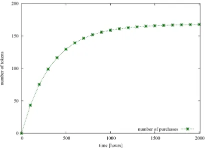
3.4 The expected value of the number of application purchases as the func- tion of elapsed time. . . 34
3.5 The expected value of the number of users who lost the interest in using the application. . . 35
3.6 The extended SPN model. . . 36
3.7 The expected value of the number of application purchases as the func- tion of elapsed time. . . 37
3.8 The expected value of the number of users who lost the interest in using the application. . . 37
3.9 The proposed operation model for the Manufacturing Process of Wooden Windows. . . 41
3.10 The number of tokens in places Coated and Joined. . . 45
3.11 The number of tokens in places Coated and Joined. . . 45
4.1 Resource contention and spectrum renting. . . 53
4.2 Illustration of state transition diagram. . . 54
4.3 Comparison with simulation (n1 =n2 = 6, 1/µ1 = 1/µ2 = 53.22s) . . . 59
4.4 Performance measures for n1 =n2 = 6, 1/µ1 = 180s and ρ2 = 0.7 . . . 60 4.5 Performance measures for n1 =n2 = 6, 1/µ1 = 180s and ρ1 = 0.8 . . . 61 4.6 Performance measures for n1 = n2 = 6, 1/µ1 = 1/µ2 = 53.22s and
ρ2 = 0.7 . . . 63 4.7 Performance measures forn1 =n2 = 6,1/µ1 = 1/µ2 = 53.22s,ρ1 = 0.85
and ρ2 = 0.7 . . . 64 4.8 Performance measures forn1 =n2 = 6,1/µ1 = 1/µ2 = 53.22s,ρ1 = 0.85
and ρ2 = 0.7 . . . 65 4.9 The APR for n1 =n2 = 3 and 1/µ1 = 1/µ2 = 108.25s . . . 66 4.10 The APR for n1 =n2 = 3, 1/µ1 = 1/µ2 = 108.25s and ρ2 = 0.575 . . . 66
List of Tables
2.1 The reachability set of SPN model of Fig. 2.4 . . . 13
3.1 The state transitions of the proposed CQN model . . . 25
3.2 Comparison of the analytical and simulation results using the CQN model 28 3.3 The state transitions of the basic SPN model. . . 32
3.4 The transitions of the DSPN model . . . 43
3.5 The token distribution of the DSPN model after one year . . . 44
4.1 Notations . . . 52
Chapter 1 Introduction
In the last few years, the number of mobile devices equipped with wireless commu- nication interfaces has increased signicantly (the ratio of the smart phones reached 26% in Hungary at the end of 2012 [22]). Besides, the number of mobile applications and the demand for broadband spectrum access show an increasing tendency, too. The change of the typical user behavior demands innovative solutions from the researchers:
alternative directions have to be oered for mobile users, which were designed according to the current trends. Accordingly, we propose a novel approach for mobile application spreading in the rst part of this dissertation; and describe our opportunistic spectrum access model for mobile cellular networks in the second part.
1.1 Motivation
In spite of the above mentioned tendency, mobile application spreading is not a frequently investigated research topic today. Traditionally, mobile applications are spread via a central entity, like an Internet web shop. Users can browse the web site of the merchant (or use a mobile market application), select, purchase and download the application they like. However, decentralized technologies such as self-organized or mobile ad hoc networks allow the users to get the application software directly from each other [16]. Hence, direct application download can change the characteristics of traditional application spreading. The participants of this direct communication can even try out the applications and be motivated to purchase the ones they liked (purchasing is available only via a traditional way, because secure payment in this environment is still a challenging issue today). In this type of communication, a lot of factors can change the characteristics of the spreading process, especially from economic viewpoint, which have not taken into consideration yet (e.g., community experience when playing a multi-player game). These factors can give more motivation to the users to purchase the application than they would have seen only some advertisements [1,2,
3, 4,5].
Another promising topic is the spectrum sharing in mobile cellular networks, typ- ically in Global System for Mobile Communications (GSM) networks, where the in- creasing demand for broadband spectrum access results in the scarcity of the available spectrum. At present, the exclusive access right to certain radio frequency bands is licensed to mobile network operators by the governments. The license of the fre- quency bands is guaranteed based on the result of spectrum auctions. However, it is already recognized that this exclusive access may lead to an inecient use of the spectrum [23, 24]. Network operators can utilize spectrum renting to increase the ef- ciency of the spectrum usage [23, 24, 25, 26, 27, 28] and to relieve the temporary capacity shortage of a particular cell in a mobile cellular network. For example, when the number of calls increases in a specic area, a network operator could decide to rent a frequency band from another operator to keep or enhance the grade of service of calls. From the service providers' point of view, it is crucial to show that besides improving the technical parameters, the cooperation is also nancially benecial for each cooperating party.
1.2 Research problem statement
With the spreading of the smart phones, more and more opportunities are oered for the users, which have been exploited only in part yet. The engineers and the developers nd innovative solutions and applications, what can open new directions in the future. However, there are still open questions, which need to be answered. In this dissertation, we deal with two problem sets.
Problem 1. Application spreading in mobile ad hoc environments. The actual form of application spreading is a centralized one. However, the distributed approach oers new ways of communications, which must not be ignored: exploiting the direct connections between the mobile devices could aect the application spreading process.
Being aware of the characteristics of application spreading is important for the appli- cation provider not only from technical, but also from economic point of view. The application provider has to know or at least assess how much money he can earn from the purchases of a given application; how much time is needed to realize it; and which factors inuence the spreading process and how [1, 2, 3, 4, 5].
Problem 2. Bottlenecks in the manufacturing process of wooden windows. In many manufacturing processes, the work can be divided into dierent disjoint phases having deterministic holding times. If a company wants to increase its production, it is advantageous to do it by the expansion of a single work phase, which is a bottleneck in the system. Therefore, it is necessary to identify the bottleneck of the manufacturing
process. Moreover, it is also desirable to determine the measure of the expansion for the elimination of the main bottleneck [7].
Problem 3. Opportunistic spectrum access in mobile cellular networks. The cur- rent regulation of spectrum licensing guarantees exclusive access to certain frequency bands for the mobile telecommunication service providers. As some recent research pa- pers have pointed out [23, 24], the exclusiveness has a negative eect on the eciency.
For the realization of a spectrum sharing system, several obstacles must be beaten o. Many researchers work in this area to solve the physical/technical problems, such as identifying the idle spectral ranges, interference problems, time and frequency syn- chronization [21]. Besides, there are still open questions if the physical diculties are got over. Since the service providers pay license fee for using the spectrum, a basic requirement is to show that another approach can protect their investments. Moreover, even an extra prot can be achieved by using spectrum sharing. The other interesting question is the quality of the service, which is mainly the mobile subscribers' interest.
Finally, the scarcity of the available spectrum will be sooner or later a great challenge for the governments.
1.3 Results
In the following, we briey present the contributions of this dissertation. We ad- ditionally give the corresponding publications and chapters of the dissertation that describe a particular contribution in detail.
Two Performance Analysis Applications Based on Deterministic and Stochastic Petri Net Models
• We proposed a Closed Queuing Network (CQN) model which can be simply used for giving an analytical lower and upper bounds on the number of application purchases.
Related publications: [1], [2], [3], [4], [5]
Chapter: 3
• We demonstrated that the mean eld based methodology can be applied for obtaining the transient solution of a Stochastic Petri Net (SPN), if the underlying Markov chain of the SPN is density dependent.
Related publications: [5], [6]
Chapter: 3
• We applied the mean eld based methodology for obtaining the transient solution of our basic SPN model, and we gave an analytical approximation on the number
of application purchases in the order of seconds.
Related publications: [5], [6]
Chapter: 3
• We proposed an extended version of the basic SPN model, for which the main properties of the application spreading process can be determined by running transient simulation.
Related publications: [5]
Chapter: 3
• Using a Deterministic and Stochastic Petri Net (DSPN) model, we identied the bottleneck of the wooden window production process and determined the measure of the extension for eliminating the main bottleneck.
Related publications: [7]
Chapter: 3
Opportunistic spectrum access in mobile cellular networks
• We elaborated a spectrum sharing policy based on the idea of opportunistic spectrum access. In the model, a high level of cooperation is realized between the mobile service providers. Besides, the model considers the current technical constraints, too, which were ignored by most of the related works.
Related publications: [8], [9], [10]
Chapter: 4
• We demonstrated via simulations that the service quality can be improved ap- plying the elaborated spectrum sharing policy. Moreover, we also demonstrated that the cooperating parties can realize more prot using our model than in the current environment.
Related publications: [8]
Chapter: 4
• We elaborated the mathematical model of the above mentioned spectrum sharing policy. We used a two-dimensional Continuous-Time Markov Chain (CTMC) to get the numerical results of the model. Since the results correspond to the simulation results, the Markovian mathematical model can be considered as a good approximation of the original model, where the channel holding times and the interarrival times are log-normally distributed.
Related publications: [10]
Chapter: 4
• We identied and measured the main drawback of our model, the forced termi- nation phenomenon. In a heavily loaded system, the forced termination increases to a level that is annoying for the mobil subscribers. To handle this problem, we elaborated a method for the protection of the ongoing calls based on the Adaptive Random Early Detection (ARED) rule [30].
Related publications: [8], [10]
Chapter: 4
1.4 Outline
The outline of this dissertation is as follows.
Chapter 2: This chapter provides a summary of the applied research methodology in the dissertation, such as queuing networks, continuous-time Markov chains and stochastic Petri nets.
Chapter 3: In this chapter, we present two performance analysis applications based on deterministic and stochastic Petri net models. In Section 3.1, we investigate application spreading in mobile ad hoc environments. We give an overview of the related works concerning application spreading in Section 3.1.1. Section3.1.2 presents a short description about how the application spreading process using ad hoc networks takes place. In Section3.1.3, we describe the communication model and dene the user behavior types. We present two techniques to investigate the application spreading process, thus our CQN and SPN models together with some results in Section 3.1.4 and Section 3.1.5, respectively. To point out the applicability of the mentioned modeling processes, we describe the operation model of a wooden window producing company and present some proposal to improve the eectiveness of the production in Section3.2. Finally, we summarize the results of the chapter in Section 3.3.
Chapter 4: This chapter describes our work in the area of opportunistic spectrum access. In Section 4.1, we give an overview about the topic with the most rele- vant related works. In Section 4.2, we present the opportunistic spectrum access model, while we describe the numerical results of the model in Section4.3. To al- leviate the negative eect of the proposed scheme, we rened the model, in which we increased the protection of the ongoing calls against the forced termination.
The rened model is discussed in Section 4.3.3. We summarize the chapter in Section 4.4.
Chapter 2
Research Methodology
This chapter provides the short overview of methodology applied to solve the prob- lems covered in the dissertation. It is worth to emphasize that performance evaluation can be carried out by dierent methods [31]:
• using a simulation software;
• by mathematical analysis with numerical procedures;
• by building the system and then measure its performance.
In this dissertation, we applied the rst and the second method for model evaluation.
Although simulation allows us to construct more sophisticated models, mathematical analysis generally needs lower computational eort [32], and produces exact solution.
2.1 Queuing Networks
Queuing networks are used for modeling systems, which can be considered as a set of interacting services.
An Open Queuing Network (OQN) can be considered as a service, which has cus- tomers from the outside world. Customers will be transferred also to the outside world after getting the service [33]. This approach is based on the fact that the arrival process can be approximately described assuming innite customer population if the number of customers is very large. In these models, the number of customers being under service does not inuence the arrival intensity of the system. Fig. 2.1 shows an example of OQNs.
A CQN has a constant number of customers circulating throughout the system.
In this model, the number of idle customers determine the arrival intensity (Fig.2.2).
This approach ensures a more precise model, and appropriate even for smaller customer
Figure 2.1: An example of open queuing networks
population. On the other hand, the analysis of these models is more challenging than in case of OQNs.
Figure 2.2: An example of closed queuing networks
In the area of queuing networks, many results were obtained in the last century [34].
These results are either exact analytical ones [35, 36] or approximations [37].
For OQNs, the Jackson networks [38, 39] have an ecient product-form solution.
For CQNs, the Gordon-Newell theorem [40] and the mean value analysis [35] can be used to obtain the exact solution. However, the above mentioned processes assume that the queuing network is well-formed, i.e., the following criteria hold [33]:
• every station is reachable from any other with a non-zero probability in case of a CQN;
• in case of an OQN, add a virtual station 0that represents the external behavior that generates external arrivals and absorbs all departing customers, so obtaining a CQN, for which the rst criterion can be applied.
In our application spreading models, the user population is nite. Therefore, using CQNs to obtain the behavior of our system is an obvious idea. However, the acyclicity of our model does not allow the use of the mentioned traditional processes, since our CQN is not well-formed (if a user purchases an application, he will never lose it again).
Therefore, we have to use other methods. By exploiting the special characteristics of the CQN model, we present an approximate analytical solution in this dissertation, while we validate the results via simulations.
2.2 Continuous-Time Markov Chains
In this dissertation, we often refer to CTMCs [41] as a fundamental modeling tool for stochastic processes. In Chapter 4, we use a CTMC for modeling opportunistic spectrum access in mobile cellular networks. In Section2.3, we will show the relation- ship between CTMCs and SPNs, which are used in Chapter3for modeling application spreading in mobile ad hoc networks. In this section, we collected the main denitions of CTMCs which are important in the remaining chapters of the dissertation.
2.2.1 The Formal Denition of CTMC
A CTMC is a stochastic process X(t)| t ≥0, t∈R such that for all t0, ..., tn−1, tn, t ∈ R,0≤t0 < ... < tn−1 < tn < t, for all n∈N
P(X(t) =x | X(tn) =xn, X(tn−1) = xn−1, ..., X(t0) =x0) =
P(X(t) =x | X(tn) = xn) (2.1)
2.2.2 Homogeneity
If we consider a discrete state space, and we denote
pij(t, s) =P(X(t+s) =j | X(t) = i) (2.2) fors >0, a CTMC is called homogenous if
pij(t, s) =pij(s) (2.3) for all t≥0.
2.2.3 Transition Rates
In a homogeneous CTMC,pij(s)is the probability of jumping from stateito statej during an interval time of duration s. The instantaneous transition rate from state i
to state j can be dened as
qij = lim
∆t→0
pij(∆t)
∆t , (2.4)
and the exit rate from state i as−qii, where qii=−X
j6=i
qij = lim
∆t→0
pii(∆t)−1
∆t . (2.5)
Q= [qij] is called innitesimal generator matrix or transition rate matrix.
2.2.4 Transient and Steady State Solution
In the following, we briey describe how to obtain the transient and the steady state probabilities of a CTMC.
• Let denoteπi(t) = P(X(t) = i)the distribution at time instantt, in matrix form P(t) = [pij(t)]. Then,π(t) = π(u)P(t−u)for u < t.
• Substituting u=t−∆t and subtracting π(t−∆t) we get
π(t)−π(t−∆t) = π(t−∆t)[P(∆t)−I], (2.6) where I is the identity matrix.
• Dividing by ∆t and taking the limit we get d
dtπ(t) =π(t) lim
∆t→0
P(∆t)−I
∆t . (2.7)
• Then, using denition of Q= [qij], we obtain the Kolmogorov dierential equa- tion [42]
d
dtπ(t) = π(t)Q. (2.8)
• The transient solution for the state probabilities π(t)can be expressed as
π(t) =π0eQt. (2.9)
• Since π(t)e = 1 with e = (1,1, ...,1), if lim
t→∞π(t) exists, then taking the limit of Kolmogorov dierential equation we get the equation for the steady state probabilities:
πQ= 0
πe= 1 (2.10)
2.2.5 A Two-State Example for CTMCs
In the second half of the last century, CTMCs were used for modeling many known systems in telecommunications. In this section, we show an example system known as M/M/1/1 system (Fig.2.3). In this simple two-state system, we assume
• innite user population with arrival rate λ,
• single server with service rate µ, and
• no buer capacity.
Figure 2.3: The M/M/1/1 system.
The corresponding innitesimal generator matrix of this system is
Q=
"
−λ λ µ −µ
#
, (2.11)
while the Kolmogorov dierential equation yields d
dtπ0(t) = −λπ0(t) +µπ1(t) d
dtπ1(t) = λπ0(t)−µπ1(t) π0(t) +π1(t) = 1
(2.12)
Given thatπ0(0) = 1, we get the transient solution as π0(t) = µ
λ+µ + λ
λ+µe−(λ+µ)t π1(t) = λ
λ+µ− λ
λ+µe−(λ+µ)t
(2.13)
Using equation (2.10), the steady state probabilities can be obtained as π0 = µ
λ+µ π1 = λ
λ+µ
(2.14)
Note that equation (2.14) can also be obtained by taking the limits as t → ∞ of equation (2.13).
2.3 The Relationship Between Continuous-Time Markov Chains and Stochastic Petri Nets
The work of several authors helped the evolution of Petri net models that led to the proposal of SPNs [43, 44]. A SPN is a Petri net extended with time handling, that makes the Petri net suitable for performance analysis purposes. The ring delays in a SPN are exponentially distributed, which is a memoryless distribution.
As we will see later in this section, it is relatively easy to show that SPNs are isomorphic to the CTMCs [45]. Therefore, the standard approach for analyzing SPNs is to construct the CTMC corresponding to the underlying stochastic behavior of the SPN [41] and perform the steady state or transient analysis analytically [46] or by simulation. The association can be obtained by applying the following rules [45]:
• The CTMC state spaceS =si corresponds to the reachability setRS(M0)of the PN associated with the SPN (Mi ↔si).
• The transition rate from state si (corresponding to markingMi) to statesj (Mj) is obtained as the sum of the ring rates of the transitions that are enabled in Mi and whose rings generate marking Mj.
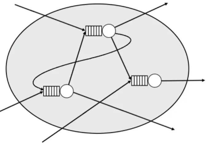
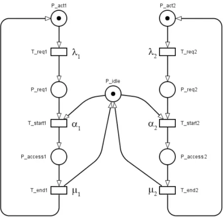
Based on these rules, the innitesimal generator (or the state transition rate matrix) of the isomorphic CTMC can be automatically constructed from the description of the SPN [45]. An example of the association is illustrated in the following. In Fig.2.4, the SPN model of shared memory system is shown, in which two processors use a common shared memory.
Omitting the detailed description, the reachability set of this system can be de- termined starting from the initial marking M0. The reachability set is presented in Table 2.1.
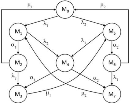
The reachability graph of a SPN denotes how the dierent markings concerning to dierent system states can be accessed. Knowing the reachability graph and the transition intensities of the SPN, it is straightforward to obtain the state transition rate diagram of the corresponding CTMC (Fig.2.5). Finally, Fig.2.6shows the innitesimal generator matrix of the system.
However, the above mentioned approach becomes unfeasible due to the size of the state space if we consider a network composed of a large number of components. In this dissertation, we describe the mean eld approach, which is a uid approximation
Figure 2.4: The SPN model of shared memory system.
Table 2.1: The reachability set of SPN model of Fig.2.4 .
M0 = P_act1 + P_idle + P_act2
M1 = P_req1 + P_idle + P_act2
M2 = P_access1 + P_act2
M3 = P_access1 + P_req2
M4 = P_req1 + P_idle + P_req2
M5 = P_act1 + P_idle + P_req2
M6 = P_act1 + P_access2
M7 = P_req1 + P_access2
method for model evaluation. Applying this method, the analysis will terminate within a few seconds, even when the state space explodes due to the high number of tokens.
This method is based on [29], while we present it in a form that is directly related to the applied denition of SPN [6]. Besides, we provide a formal relation between the CTMC and its uid approximation in Chapter3.
Unfortunately, if a SPN model contains inhibitor arcs, the uid approximation method is not feasible. Instead, simulation can be used to evaluate the model. The simulation of stochastic Petri nets is supported by many known tools, like the ones presented in [47, 48, 49].
Figure 2.5: The state transition rate diagram of the CMTC associated with the SPN in Fig. 2.4.
Figure 2.6: The innitesimal generator matrix of the CTMC in Fig. 2.5.
2.4 Deterministic and Stochastic Petri Nets
In a manufacturing process, the work phases have deterministic delay. A process, in which the delays of the transitions are either exponentially, or deterministically distributed, can be appropriately described by a DSPN [50]. DSPNs are similar to SPNs, except that deterministically delayed transitions are also allowed in the Petri net model.
Although DSPNs have greater modeling strength than SPNs, there are some re- strictions in the model evaluation phase. However, Lindemann and Shedler [51], and Lindemann and Thümmler [52] showed that in some special cases, the DSPNs can be
handled analytically even with concurrently enabled deterministic transitions, the nu- merical analysis of DSPNs are generally limited to the case when there is at most one enabled deterministic transition in each marking (for further details, see Section3.2).
In these cases, simulation can be used to get the steady state or the transient solution of the DSPN. The simulation of DSPNs is supported by many known tools, e.g. by TimeNet [47].
2.5 Simulation
In this dissertation, several simulation results are presented. This section provides a short overview about the simulation of stochastic processes.
2.5.1 Discrete-Event Simulation
Discrete-event simulation is used for modeling a system which can change at only a countable number of points in time. Events occur in these points, where an event is dened as an instantaneous occurrence that may change the state of the system [53].
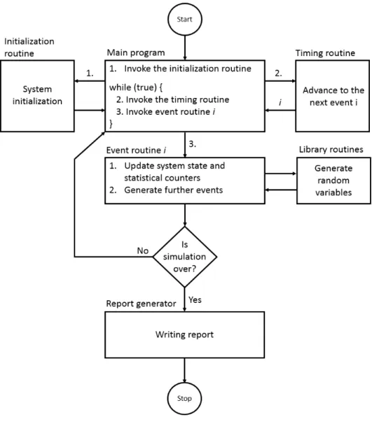
In each discrete-event simulation, a variable called simulation clock stores the cur- rent value of the simulated time. In this dissertation, we follow the next-event time- advance approach. The simulation clock is initialized to zero, and we determine the future events and their times of occurrence. Then, the simulation clock is advanced to the rst future event, when the system is updated, the future events and their times of occurrence are determined again, and so on. The simulation process terminates when an investigated variable reaches a predened value (e.g. the simulation clock reaches its predened maximal value).
In most discrete-event simulation software, the following components can be found [53].
• System state: The set of state variables, which describe the system.
• Simulation clock: A variable for storing the current value of simulated time.
• Event list: A list of events containing the next time of occurrence of each event.
• Statistical counters: Variables for storing statistical information about the sys- tem.
• Initialization routine: A function for initialize the system before the simulation starts.
• Timing routine: A function that determines the next event in the event list and advances the simulation clock to the time of occurrence of that event.
• Event routine: A function for updating the system when a particular type of event occurs.
• Library routines: A set of functions for generating random observations from probability distributions.
• Report generator: A function for producing a report when the simulation termi- nates.
• Main program: The main program invokes the timing routine, checks for termi- nation and invokes the report generator when the simulation is over.
The discrete-event simulation process is illustrated in Fig.2.7 [53].
Figure 2.7: The ow chart of discrete-event simulation process.
2.5.2 Generating Random Variables
Usually, simulation processes have random aspects, which involves the demand for generating random variables from probability distributions. For this task, it is essen- tial to have a reliable pseudo-random number generator function producing random numbers with uniform distribution inU[0,1). Then, random numbers with the desired probability distribution can be generated as follows:
• Generate a pseudo-random number in U[0,1).
• Let ξ a variate with probability distribution Fξ(x) = P(ξ < x).
• If U ∈[0,1)has uniform distribution, then the ξ =Fξ−1(U) variate is a random variable with probability distribution Fξ(x).
Example: Let be Fξ(x) =P(ξ≤x) = 1−e−λx. Then
ξ =Fξ−1(U) =
ln( 1 1−U)
λ =
ln( 1 U1)
λ , (2.15)
whereU1 ∈[0,1)is a variate with uniform distribution.
2.5.3 The Precision of Simulation
For determining the precision of simulation, interval estimation is a commonly used technique.
P(|¯γ(n)−E[γ]| ≤∆) = 1−α, (2.16) where
• 1−α is the condence level,
• ∆ is the half-width of the condence interval, and
• = ∆/¯γ is the relative precision.
Ifn is suciently large, then
∆(n) = z1−α/2σˆγ(n), (2.17) wherez1−α/2 is the (1−α/2)quantile of the standard normal distribution.
It is also known, that if the deviation of variate γ is σγ, then the deviation of n experiment σγ(n):
σγ(n) = σγ
√n (2.18)
Therefore, in case of n2 experiments,
• the deviation of the result decreases to its nth,
• the width of the condence interval also decreases to its nth.
Chapter 3
Two Performance Analysis
Applications Based on Deterministic and Stochastic Petri Net Models
But innovation comes from people meeting up in the hallways or call- ing each other at 10:30 at night with a new idea, or because they realized something that shoots holes in how we've been thinking about a problem.
(Steve Jobs)
In this chapter, we oer an alternative approach for the application providers to spread an application exploiting the direct communication between the users. Based on our proposed communication model and user types, we present dierent models and techniques for obtaining results regarding to the application spreading process. Besides, we show that our applied modeling techniques can be used in the wood industry, too, where we describe a wooden window manufacturing process with a DSPN model.
The outline of the chapter is as follows. Section 3.1 presents a CQN and two SPN models for application spreading in mobile ad hoc environments. In the evaluation of these models, dierent techniques are used depending on the complexity of the models.
In Section 3.2, we model the wooden window manufacturing process with a DSPN to demonstrate that the stochastic models can be applied in the wood industry. Finally, we summarize this chapter in Section3.3.
3.1 Application Spreading in Mobile Ad hoc Environ- ments
In this section, we present our mobile application spreading models. We emphasize that our communication model described in Section 3.1.3 works in an environment,
which possibly will exist, since the proliferation of ad hoc networks is not guaranteed today. Therefore, the validation of our results is also a dicult question. However, our approach will surely not exist if no one shows that it can work (the situation is similar to the chicken-and-egg problem). On the other hand, some innovative proposals like the multi-touch screen of the smart phones had also seemed meaningless for many experts until someone built them and met with success. In the current phase, our work described in this section can be considered as a pioneer one, which can be a base of further works in this area.
In Section3.1.1, we give a short overview about the related works. In Section3.1.3, we describe our communication model and present the user types, which we assume in our models. Section3.1.4presents the CQN model, which can be simply used for giving an analytical estimation on the number of application purchases. For obtaining more sophisticated results, we present two SPN models in Section 3.1.5. In the rst SPN model, the underlying CTMC must be density dependent in order to apply a mean eld based methodology, which provides an analytical approximation of the transient solution of the SPN. In the second model, we can handle a ner model, since the underlying CTMC of the SPN does not have to be density dependent. However, we have to use simulation to obtain the solution of the SPN.
3.1.1 Related Works
With the proliferation of modern communication paradigms, the investigation of application spreading using new ways becomes more and more important. However, it has not got too much attention so far. Besides our previous contributions [1, 2, 3, 4, 5, 6], only a few papers touch even the commercial use of ad hoc networks and direct communication.
On the other hand, epidemic spreading is a popular research topic today and this area is similar to the context of application spreading. In [54], the authors present a model, by which they investigate the propagation of a virus in a real network. In [55], the authors present scale-free networks for modeling the spreading of computer viruses and also give an epidemic threshold, which is an infection rate. Information spreading is also investigated by using epidemic spreading models, such as the Susceptible-Infected- Resistant (SIR) model [56], or other models based on the network topology [57, 58].
In [59], malicious software spreading over mobile ad hoc networks is investigated. The authors propose the use of the Susceptible-Infected-Susceptible (SIS) model based on the theory of Closed Queuing Networks. In [60], the authors propose the commercial use of ad hoc networks and present a radio dispatch system using mobile ad hoc com- munication. In the proposed system, the connectivity of the nodes is the key element of information dissemination.
In our models, we do not consider the network topology as a key element of appli- cation spreading, since no real-time information dissemination is needed between the users. For the same reason, we do not deal with mobility models such as random walk model, which are well presented in many contributions [61, 62, 63].
Although the above mentioned proposals show some similarities with our work, none of them deals with application spreading and, except [60], they do not touch the commercial benets of direct communication. Moreover, the authors in [60] consider information dissemination as a tool, and not as a goal.
3.1.2 The Application Spreading Process using Mobile Ad Hoc Connections
Nowadays, nearly all mobile devices have got at least one wireless interface (e.g.
Wi-Fi), which is appropriate for ad hoc communications. Ad hoc networks oer a good opportunity to communicate even when no central infrastructure is available. However, this advantageous property implies some diculties, too. First, the communication range is limited due to the limited strength of the emitted signal in the Industrial, Scientic and Medical (ISM) band. Furthermore, the lack of business interest (no internet service provider is needed) does not facilitate the software development for ad hoc environments. Finally, the lack of central entities makes the network conguration more dicult.
On the other hand, the short communication range involves some advantages, too.
For example, the community experience of a multi-player game is signicantly increased in a Local Area Network (LAN) environment, where the players can hear and/or see each other. However, LAN games are popular even now, they are available mostly in a pre-congured environment with xed location, typically using desktop computers.
Our approach is a more general extension of LAN applications, since the location is not xed. However, the above mentioned conguration problem still exists. To ease the network management in ad hoc networks, a service provisioning framework is proposed in [16]. Using the framework, the nodes discover each other, and have the opportunity to make services available for other nodes. Besides, the framework can alleviate the conguration diculties.
Our approach assumes that meeting points will be formed, where people who want to use multi-user applications can nd each other, and can form ad hoc networks. The network can be maintained even with low number of users, too, and is not sensitive to the relatively frequent topology changes caused by the appearing and disappearing of nodes.
3.1.3 Communication Model and User Types
In this section, we present the communication model which we use in our investi- gations. Moreover, we introduce three user types based on dierent user behaviors.
Communication Model
We refer to the individuals who are interested in the use of the application as users. The population that we investigate is composed of users only, and we do not take uninterested users into consideration, because they do not inuence the spreading process. Therefore, we assume a closed user population.
We investigate the spreading of a given multi-user application having two versions, a trial and a full version. The users can be categorized into dierent classes depending on whether they do possess any version of the given application or do not. We named the classes after the terminology of epidemics, since our model shows similarity to the epidemic spreading models. A user is called i)infected, if he has got the full version of the application; ii)susceptible, if he possesses only the trial version of the application;
and iii) resistant, if he has got none of them, or he has already lost the interest of using the application.
Users with their mobile devices form self-organized networks from time to time, in which direct communication takes place. The trial version of the application is free and available in these networks, so users can download it and even try it out. However, it has some restrictions (see later), so the users have to purchase the application for unrestricted usage via a traditional way of purchasing. Later, also these users can spread the trial version of the purchased application further.
Since application providers want susceptible users to be motivated in purchasing the full version of the application, some limitations must be made in using the trial version.
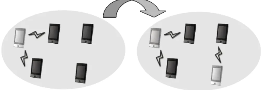
Therefore, we apply a limit (leech1 limit) that restricts how many nodes possessing the trial version (leech1) can connect to a node possessing the full version (seed1). In this sense, the seeds can be considered as servers, which can serve a limited number of clients. A seed is always an infected user, while a leech may be either infected or susceptible. Fig.3.1depicts the case when a susceptible user purchases the application.
The devices form an ad hoc network, in which the dark devices depict susceptible users, while the light ones depict infected users. In this example, the leech limit is two, so two susceptible users can peer to the only infected user, while the other two have to wait (the connection symbol represents application level peering). After one of them purchased the application, they can also use it, as shown in the right side of Fig. 3.1.
1After the terminology of BitTorrent [64]
Figure 3.1: Change of application usage when a susceptible user purchases the appli- cation.
User Types
Beyond the basic communications, we distinguish three dierent user types based on the users' behavior.
• T ypeA users are interested in using the given application. Therefore, they are its potential buyers even without trying it out.
• T ypeB users also purchase the application very likely, but they will do it with a given intensity, only if they cannot nd a seed from time to time which they can connect to.
• T ypeC users instead will never purchase the application but still they inuence the spreading process because they decrease the probability that other users nd an available seed to connect to.
In our CQN model, all the three types of users are present, and we can give a lower and an upper bound for the expected number of application purchases analytically. In our basic Petri net model, we use the mean eld approach to obtain analytical results.
However, our basic Petri model cannot handle theT ypeB users, since their behavior's description results in the violation of the density dependent property in the underlying CTMC of the SPN. Therefore, we omit T ypeB users from the basic model. In our extended Petri net model, we can handle the presence of T ypeB users, too, but only using transient simulation. Of course, additional user types can be introduced, too.
However, the more user types we capture the more complex model we get, which can make the handling of the model dicult.
3.1.4 Modeling with Closed Queuing Networks
In self-organized networks, where spontaneous communication takes place, the net- work topology can change rapidly due to the high degree of mobility. These topology
changes can be modeled by stochastic processes [65]. We can appropriately describe a stochastic process in a closed population, which is interesting from our point of view, using CQNs [34]. Moreover, ordering transition intensities to the state changes we can capture the time behavior of the application spreading process, too.
Spreading Model
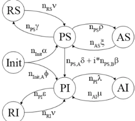
For modeling the application spreading with CQNs, we propose the model depicted in Fig. 3.2. In this CQN model, the dierent states represent the whole user popula- tion. Each user is in one state depending on his current user class. Resistant users which possess neither the full version nor the trial version of the application are in state Init. We call also resistant the users, who have already lost the interest in using the application. However, they possess either its trial (state RS) or its full version (state RI). The susceptible users are in state P S and AS, depending on that they are currently using the application (Active Susceptibles, AS) or not (Passive Suscep- tibles, P S). Similarly, the active and passive infected users are in state P I and AI, respectively.
Figure 3.2: The proposed CQN model.
The Greek letters in Fig.3.2denote transition intensities regarding to a single user, nx represents the number of users in state x, while nx,A, nx,B and nx,C represent the number of T ypeA,T ypeB and T ypeC users in state x, respectively (nx =nx,A+nx,B+ nx,C). The transition intensity is a real number assigned to the state transition, which denotes how many times a state transition takes place during a given time interval.
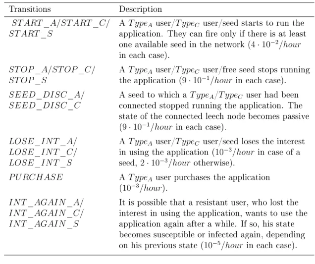
These transitions are described in Table 3.1.
Usage of the Spreading Model
We can unambiguously describe the state of the system with the user distribution (nInit, nP S, nAS, nP I, nAI, nRS, nRI). The transition intensities (α, β, γ, δ, , φ, λ,
Table 3.1: The state transitions of the proposed CQN model
Transitions Description
P S →AS A susceptible user starts to run the application and tries to connect to a seed in the network. If he cannot nd one, he has to wait.
AS →P S A susceptible user stops running the application.
P I →AI An infected user starts to run the application, then either he tries to connect to an available seed, or will be a seed himself to which leeches can connect.
AI →P I An infected user stops running the application.
Init→P S A resistant user downloads the trial version of the application.
P I→RI An infected user becomes resistant losing the interest in using the application.
P S →RS A susceptible user becomes resistant losing the interest in using the application.
Init→P I A resistant user purchased the application without trying it out.
P S→P I A susceptible user becomes infected by purchasing the application.
A susceptible user purchased the application. nP S,A and nP S,B denote the number ofT ypeA and T ypeB users in state P S, respec- tively. This transition is enabled only for T ypeB users when there is no free seed available in the network which they can connect to.
Therefore, the indicator variablei is zero if there is no free seed available, and one otherwise. T ypeC users never purchase the application, so this state transition is not allowed to take place for T ypeC users. However,T ypeC users can also connect to seeds, so decreasing the probability that other users nd a free seed which they can connect to.
RS →P S It is possible that a resistant user, who lost the interest in using the trial version, wants to use the application again after a while.
If so, his state becomes susceptible again.
RI →P I Similarly, if a resistant user possessing the full version of the application wants to use it again, his state changes to infected.
µ, ν,ρ and ξ) regarding to a single user are the system parameters, which are hard to be determined theoretically. In this dissertation, we set the system parameters based on common sense. The parameter setting can be ne-tuned experimentally, what is beyond the scope of this dissertation.
In each system state, we can generate the holding timeh(the time that the system is expected to spend in a given system state) as an exponentially distributed random
variable2 in the following way:
h= −lnRN D X
∀state x
outx
, (3.1)
where 0 ≤ RN D < 1 is a pseudo-random number, and outx denotes the sum of the intensities for each transition with source state x. We must compute h after each state change, because the user distribution changes when a transition takes place. We generate the next system state based on the ratio of the current transition values. After we generated the transition that takes place, we move one user from its source to its destination state, then compute the holding time of the new system state, and so on.
At the beginning, each user is in stateInit, which is the initial state of the system.
The users will leave this state and change their states from time to time. After a while, a user will lose the interest in the application usage (reaches state RS or RI), but it does not mean that he cannot be interested again later on. Thus, the state transitions RS →P SandRI →P Iare also enabled, however, it is allowed only with low intensity values for them. Therefore, we will reach a system state (rest state) at time instant τ, in which each user is either in stateRS orRI. The rest state can be dened as follows:
Denition 1 The system is in rest state, if for ∀state x6∈ {RS, RI}, nx = 0.
The rest state is not the steady state, however, our investigation will stop here.
Taking into account the asymmetry of this system (if someone purchases the applica- tion, he will never lose it), each user will be in one of state RI, P I or AI by reaching the steady state (even product-form solution exists). However, it is meaningless to consider this state in the model investigation, since after reaching the rest state, the holding times become extremely large, so the system changes very slowly. Hence, our investigations are always transient and consider only a time period which is interesting from the merchant's point of view.
We can determine how many pieces of the application were sold, upon reaching the rest state, by summing the number of P S →P I and Init→P I transitions. Running simulations and evaluating the results, we can observe the time characteristics of the spreading process, too.
Results Derived from CQN
In this section, we describe some analytical results [4] and validate them via simu- lations.
2Using exponentially distributed holding times is a usual modeling simplication in this context [59, 66]
Analytical solutions of CQNs can be obtained, e.g., with the well-known Mean Value Analysis (MVA) [35]. However, we investigate the transient behavior of the system, in which case this method is not feasible.
After a while, each user will leave the initial state, since we do not take the un- interested individuals into consideration. Based on the intensity value of transition Init → P I and Init → P S, we can determine how many users will expectedly pur- chase the application without trying it out (direct purchases, DP(τ)) in the following way:
DP(τ) = nInit,A· φ
α+φ, (3.2)
where nInit,A denotes the initial number of T ypeA users in state Init, i.e., the total number of T ypeA users, and τ denotes that the number of direct purchases concerns to the time instantτ, when the system reaches its rest state. As we mentioned before, we consider onlyT ypeA users when computing DP(τ). All nodes (users) that did not purchase the application without trying it out will change their state to susceptible.
Susceptible states are state P S and AS, and there are two possibilities for the users to leave these states: a user can become either (1) resistant (transition P S→RS); or (2) infected (transition P S → P I). Moreover, it is also allowed to return from state RS, but the intensity of transition RS → P S is very low, since losing the interest and being interested again after a while is not a typical user behavior. Therefore, we estimate the number of indirect purchases (purchase after trying out) based on the ratio of transitionP S→P I and P S→RS. In case of the rest ofnA−DP(τ)T ypeA users, IDPA(τ)concerning to the time instant τ can be computed as
IDPA(τ) =nInit,A· α
α+φ · δ
δ+γ, (3.3)
while we can give an upper bound on the purchases of T ypeB users concerning to the time instant τ as
IDPB(τ)≤nB· β
β+γ, (3.4)
where equality holds only if the indicator variable i is equal to one.
Summing equations (3.2) and (3.3), we can give a lower bound on the total number of purchasesT P(τ), while we can give an upper bound onT P(τ)by summing equations (3.2), (3.3) and (3.4):
DP(τ) +IDPA(τ)≤T P(τ)≤DP(τ) +IDPA(τ) +IDPB(τ), (3.5) whereτ denotes that this result also concerns to the rest state of the system.
To validate the analytical results we ran simulations. Table 3.2 compares the an-
alytical results to the average of 10000 individual simulation runs with the following parameters: nInit,A = nInit,B = nInit,C = 500, α = 10−3, β = 10−3, γ = 2 ·10−3, δ = 10−3, = 10−3, φ = 10−5, λ= ρ= 4·10−2, µ=ξ = 9·10−1, ν = 10−9, while the leech limit was one.
Table 3.2: Comparison of the analytical and simulation results using the CQN model
Description Analytically By simulation
DP(τ) 4.95 4.95
IDPA(τ) 165.02 164.99
IDPB(τ) IDPB(τ)≤166.67 36.74 T P(τ) 169.97≤T P(τ)≤336.64 206.68
Further properties, such as the time behavior of the spreading process can be in- vestigated also via simulations.
3.1.5 Modeling with Stochastic Petri Nets
In this section, we present the description and the analysis of two SPN models after introducing the fundamentals of Stochastic Petri Nets [45]. With the basic and the extended SPN model, we will be able to handle also T ypeB andT ypeC users' presence.
SinceT ypeA users are present in all of our models (including the CQN model), we compare the models from the viewpoint of this simple user behavior, see Section 3.3.
SPN Formalism
In this section, we provide a brief introduction to SPNs, while a detailed introduc- tion with applications can be found in [45].
SPNs are bipartite directed graphs with two types of nodes: places and transitions.
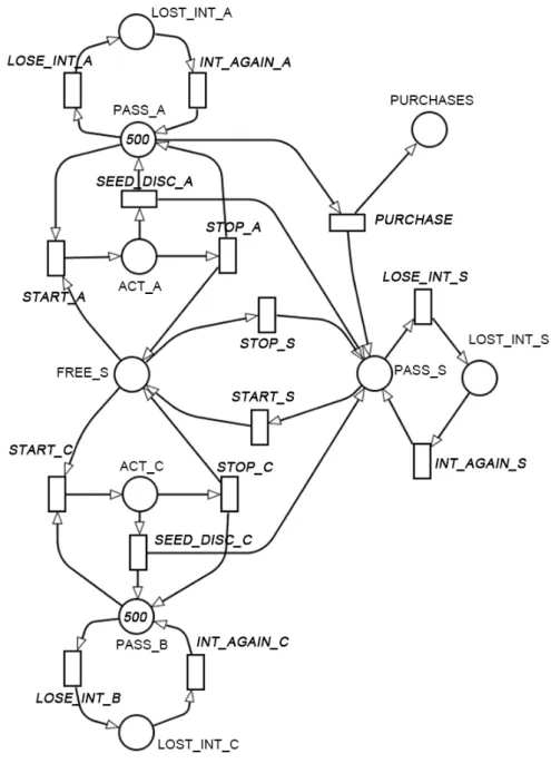
An example of a SPN is the one depicted in Fig. 3.3. The places, graphically repre- sented as circles, correspond to the state variables of the system; while the transitions, graphically represented as boxes, correspond to the events that can induce a state change. Examples of places for the SPN in Fig. 3.3 are ACT_A and ACT_B; while examples of transitions are ST OP_A and ST OP_B. The arcs connecting places to transitions and vice versa express the relation between states and event occurrence.
Places can contain tokens drawn as black dots within places. The state of a SPN, called marking, is dened by the number of tokens in each place. In this dissertation, we use the notation M to indicate a marking in general. We will denote by M(p) the number of tokens in place p in marking M. Now we recall the basic denitions that are necessary for the rest of the chapter.
Denition 2 An SPN system is a 6-tuple
(P, T, I, O, λ, M0),
where:
• P ={pi} is the set of places of cardinality k;
• T ={ti} is the set of transitions of cardinality m;
• I, O :T ×P →IN are the input and output functions that dene the arcs of the net and their multiplicities;
• λ :T →IR is the function that assigns to each transition its ring intensity;
• M0 is the initial marking of the net.
A transition is enabled if each of its input places contains the necessary amount of tokens where necessary is dened by the input function I. Formally, transition t is enabled in marking M if for all places p of the net we have M(p) ≥ I(t, p). For example, transition ST ART_A in Fig. 3.3 is enabled if the current marking contains at least one token in place P ASS_A and at least one token in place F REE_S. An enabled transition can re and the ring removes tokens from the input places of the transition and puts tokens into the output places of the transition. The new marking M0 after the ring of transition t is formally given M0(p) = M(p) +O(t, p)−I(t, p),
∀p∈P.
The ring of a transition occurs after a random delay. The random delay associated with a transition has exponential distribution whose parameter depends on the ring intensity of the transition and on the actual marking. In this section, we assume that the more tokens enable a transition the faster the transition res. This concept, called innite server policy, is captured formally by the denition of the enabling degree.
Denition 3 The enabling degree of transition t in marking M, denoted by ed(t, M), isd i ∀p∈P, M(p)≥dI(t, p) and ∃p∈P :M(p)<(d+ 1)I(t, p).
For instance, if there are three tokens in place P ASS_A and four tokens in place F REE_S then the enabling degree of transition ST ART_A is three. The random delay associated with transition t in markingM is exponentially distributed with pa- rameter λ(t)ed(t, M). When a marking is entered, a random delay is chosen for all enabled transitions by sampling the associated delay distribution. The transition with the lowest delay res and the system changes marking.