3 Spreading linear triple system

Spreading linear triple systems and expander triple systems

Zoltán L. Blázsik^∗, Zoltán Lóránt Nagy^†

MTA–ELTE Geometric and Algebraic Combinatorics Research Group Eötvös Loránd University, Budapest, Hungary

Department of Computer Science

H–1117 Budapest, Pázmány P. sétány 1/C, Hungary blazsik@caesar.elte.hu, nagyzoli@cs.elte.hu

Abstract

The existence of Steiner triple systems STS(n)of ordern containing no nontrivial sub- system is well known for every admissible n. We generalize this result in two ways. First we define the expander property of3-uniform hypergraphs and show the existence of Steiner triple systems which are almost perfect expanders.

Next we define the strong and weak spreading property of linear hypergraphs, and de- termine the minimum size of a linear triple system with these properties, up to a small constant factor. This property is strongly connected to the connectivity of the structure and of the so-called influence maximization. We also discuss how the results are related to Erdős’

conjecture on locally sparseSTSs, influence maximization, subsquare-free Latin squares and possible applications in finite geometry.

Keywords: linear hypergraph, Steiner triple system, expander, connectivity, extremal graphs, partial linear space

1 Introduction

A Steiner triple system S of order n, briefly STS(n), consists of an n-element set V and a collection of triples (or blocks) of V, such that every pair of distinct points in V is contained in a unique block. It is well known due to Kirkman [19] that there exists an STS(n) if and only ifn≡1,3 (mod 6), these values are calledadmissible. Steiner triple systems correspond to triangle decompositions of the complete graphG=K_n. In the context of triangle decompositions of a graph G, an edge will always refer to a pair of vertices which is contained in one triple of a certain triple system, E(G) denotes the edge set of G, while |S| is the number of triples in the system, which obviously equals ¹₃|E(G)|in the case of triple systems obtained from triangle decompositions of a graph G.

A triple system induced by a proper subsetV⁰ ⊂V consists of those triples whose elements do not contain any element ofV \V⁰. A nontrivial Steiner subsystem ofS is anSTS(n⁰)induced by a proper subset V⁰ ⊂V, with|V⁰|=n⁰ >3. Speaking about any triple system’s subsystem, we always suppose that it is of order greater than3. Similarly but not analogously, we call a subset

∗The research was supported by the Hungarian National Research, Development and Innovation Office, OTKA grant no. SNN 132625.

†The author is supported by the Hungarian Research Grants (NKFI) No. K 120154 and SNN 132625 and by the János Bolyai Scholarship of the Hungarian Academy of Sciences

V⁰ ⊂V of the underlying set of a triple systemF nontrivial if it has size at least 3and it is not an element of the triple system. Our aim is to generalize and strengthen the results concerning the subsystem-free property of Steiner triple systems, and in general, linear triple systems. This general concept in incidence geometry is also studied and they are called partial linear spaces.

This paper is devoted to the study of two main features of linear triples systems in an extremal hypergraph theory aspect. The first property is the expander property while the second is the so-calledspreading property.

In 1973, Erdős formulated the following conjecture.

Conjecture 1.1 (Erdős, [13]). For every k ≥ 2 there exists a threshold nk such that for all admissible n > n_k, there exists a Steiner triple system of order n with the following property:

every t+ 2 vertices induce less thant triples of S for 2≤t≤k.

This conjecture is still open, although recently Glock, Kühn, Lo and Osthus [17] and indepen- dently Bohman and Warnke [5] proved its asymptotic version. In other words, this conjecture asserts the existence of arbitrarily sparse Steiner triple systems.

One should note here that it is also a natural question whether typical Steiner triple systems are sparse in a very robust sense, namely that they do not contain Steiner subsystems. Indeed, this is equivalent to avoiding a set of t < n vertices inducing quadratically many, ¹_{3 2}^t

triples.

The first result in this direction was due to Doyen [10], who proved the existence of at least onesubsystem-free STS(n)for every admissible order n. In the language of triangle decomposi- tions of the edge set, a subsystem-free STSmay be seen as a decomposition where every subset V⁰ ⊂V(G) contains at least one edge which belongs to a triangle not induced by V⁰. In order to capture this phenomenon and its generalisation, we require some notation and definitions.

Definition 1.2. Given a3-uniform linear hypergraph F (i.e. linear triple system), let E(F) be the collection of vertex pairs (x, y) for which there exists a triple (x, y, z) from the system F, containing x and y. The corresponding graph G(F) is referred to as the shadow or skeleton of the system.

Definition 1.3 (Closure and spreading property). Consider a graph G =G(V, E) that admits a triangle decomposition. This decomposition corresponds to a linear triple system F. For an arbitrary set V⁰ ⊂V,N(V⁰) denotes the set of its neighbours:

z∈N(V⁰)⇔z∈V \V⁰ and ∃xy∈E(G[V⁰]) :{x, y, z} ∈ F.

The closure cl(V⁰) of a subset V⁰ w.r.t. a (linear) triple system F is the smallest set W ⊇ V⁰ for which |N(W)|= 0 holds. Note that the closure uniquely exists for each set V⁰. We call a (linear) triple system F spreading if cl(V⁰) =V for every nontrivial subsetV⁰ ⊂V.

Consequently, a STS(n) is subsystem-free if and only if |N(V⁰)| > 0 holds for all nontrivial subsetsV⁰ of the underlying setV of the system. Note that Doyen used the termnon-degenerate plane for STSs with the spreading property [10, 11].

Two natural extremal questions arise here. The first one concerns the lower bound on |N(V⁰)|

in terms of|V⁰|in the case of Steiner triple systems, while the second one seeks for edge-density conditions on triangle decompositions of general graphs G=G(V, E), i.e. linear triple systems, where the condition|N(V⁰)|>0 must hold for all nontrivial subsets ofV.

Problem 1.4 (Expander STSs). Let us call a Steiner triple system ε-expander if there exists someε >0 such that for every nontrivial V⁰ ⊂V(G), ^|N(V_|V0|^0)| ≥ε holds provided that|V⁰| ≤ ^|V₂^|. Does there exist an infinite family of ε-expander Steiner triple systems STS(n) for some ε >0?

How large ε >0 can be?

This can be interpreted as the analogue of the expander property of graphs and the vertex isoperi- metric number [1]. Similar generalized concepts for expanding triple systems were introduced very recently by Conlon and his coauthors [7, 8], see also the related paper [15]. Observe however that their definition is slightly different for a triple system to be expander, as Conlon defines the edge-, resp. triple-neighbourhood of a subsetF to be the edges of the skeleton not contained in F which determine a triple with a point in F, or triples not induced byF which has a point in F, respectively.

Problem 1.5 (Sparse spreading linear triple systems). What is the minimum size ξsp(n) of a linear spreading triple systemF on n vertices?

For these triple systems, the closure of any nontrivial subset with respect to the underlying graph of the triple system is the whole system.

Note that one might require only a weaker condition, namely that the closure of any nontrivial subset of the triple systemF(i.e. consisting of at least two triples) should be the whole system. In applications this condition is equally important, since it models whether every set of hyperedges has a direct influence on the whole system. For this concept, we introduce the following notation.

Notation 1.6. A triple system F is weakly spreadingif cl(V⁰) =V holds for every V⁰ =V F⁰

: F⁰ ⊆ F, |F⁰|>1.

It is easy to see that one gets the same concept if the conditioncl(V⁰) =V is required for every V⁰ = V (F⁰) for which ∃F⁰ ⊆ F, |F⁰| = 2. On the other hand, the condition cl(V⁰) = V is essential in the sense that cl(V⁰)⊃V is a much weaker property, see Construction 4.6.

Problem 1.7(Sparse weakly spreading linear triple systems). What is the minimum sizeξwsp(n) of a linear weakly spreading triple system F on n vertices?

Our main results are as follows.

Theorem 1.8. For odd prime number p, there exists a Steiner triple system STS(3p) of order 3p, for which

|N(V⁰)| ≥ |V⁰| −3 for every V⁰ ⊂V(G) of size|V⁰| ≤ ^|V₂^|.

The result is clearly sharp sinceV⁰ can be chosen to be the elements of a triple.

Corollary 1.9. For every sufficiently large n, there exists a Steiner triple system STS(n) of order n, for which

|N(V⁰)| ≥ |V⁰| −3

for every V⁰ ⊂ V(G) of size |V⁰| ≤ ^|V₂^|, where n ∈ [n−n^0.525, n] due to the result of Baker, Harman and Pintz on the difference between consecutive primes [3]. Consequently, for every n one can find a Steiner triple system S of size |S| = (1 +o(1))ⁿ₆² which is almost 1-expander.

Indeed, we may simply take a construction via Theorem 1.8 for a prime p∈[n−n^0.525, n].

As we will see, much smaller edge density compared to that ofSTSs still enables us to construct spreading linear triple systems.

Theorem 1.10. For the minimum size of a spreading linear triple system, we have 0.1103n²−O(n)< ξsp(n),

while

ξsp(n)<

5

36 +o(1)

n²≈0.139n²

holds for infinitely many n.

Surprisingly, the weak spreading property does not require a dense structure at all.

Theorem 1.11. For the minimum size of a weakly spreading linear triple system, we have n−3≤ξ_wsp(n)< 8

3n+o(n).

The paper is organised as follows. Section 2 is devoted to the expander property of Steiner triple systems and related questions. In Section 3, we make a connection between k-connectivity of 3-graphs and the spreading property, and prove Theorem 1.10 and Theorem 1.11. Finally, in Section 4 we discuss related problems concerning Latin squares and influence maximization, and possible applications, notably in the field of finite geometry.

2 Expander property of Steiner triple systems

In order to prove Theorem 1.8, we recall first the STS construction of Bose and Skolem for n = 6k+ 3 where 2k+ 1 is a prime number, and the well-known Cauchy-Davenport theorem with its closely related variant, the result of Dias da Silva and Hamidoune about the conjecture of Erdős and Heilbronn. We refer to the book of Tao and Vu [23] on the subject.

Theorem 2.1 (Cauchy-Davenport). For any prime p and nonempty subsets A and B of the prime order cyclic group Zp, the size of the sumset A+B ={a_i+bj | ai ∈ A, bj ∈ B} can be bounded as |A+B| ≥min{p, |A|+|B| −1}.

Theorem 2.2 (Erdős-Heilbronn conjecture, Dias da Silva and Hamidoune ’94). For any prime p and any subset A of the prime order cyclic group Zp, the size of the restricted sumset A+A˙ = {a_i+aj |ai 6=aj ∈A} can be bounded as |A+A| ≥˙ min{p, 2|A| −3}.

Construction 2.3(Bose and Skolem, casen= 6k+ 3). Let the triple systemS be defined in the following way. The underlying set is partitioned into three sets of equal sizes,V(S) =A∪B∪C, where |A|=|B|=|C|= 2k+ 1. Elements of each partition class are indexed by the elements of the additive group Z2k+1. The systemS contains the triple T, if

• T ={a_i, bi, ci}, i∈Z2k+1, or

• T ={a_i, a_j, b_k}, i6=j ∈Z2k+1, k= ¹₂(i+j), or

• T ={b_i, b_j, c_k}, i6=j∈Z2k+1, k= ¹₂(i+j), or

• T ={c_i, cj, a_k},i6=j∈Z2k+1, k= ¹₂(i+j).

See [22] for further details and generalisations.

Proof of Theorem 1.8. Let us apply Construction 2.3 with p= 2k+ 1prime. Consider a subset V₀=A₀∪B₀∪C₀ of the underlying setV(S) =A∪B∪C, where|V₀| ≤ ⁿ₂. In order to bound N(V0), we prove a lower bound onV0∪N(V0). Observe that a vertexv belongs toN(V0)if and only if there exist two elements of V0 together with which it forms a triple of S. Let us denote by A^∗, B^∗, C^∗ the restrictions of V₀∪N(V₀) to the partition classes A, B, C. The structure of Construction 2.3 and Theorems 2.1 and 2.2 in turn implies the following sets of inequalities of Cauchy-Davenport and Erdős-Heilbronn type, respectively.

|A^∗| ≥min{p, | −A0|+|B₀| −1} if |A₀|,|B₀|>0,

|B^∗| ≥min{p, | −B0|+|C₀| −1} if |B₀|,|C₀|>0,

|C^∗| ≥min{p, | −C₀|+|A₀| −1} if |C₀|,|A₀|>0.

(2.1)

|A^∗| ≥min{p, 2|C₀| −3},

|B^∗| ≥min{p, 2|A₀| −3},

|C^∗| ≥min{p, 2|B₀| −3}.

(2.2)

Note that in the Erdős-Heilbronn type inequalities (2.2), the lower bound can be improved by one if the set consists of a single element. We distinguish several cases according to the sizes of the sets A0, B0, and C0.

First suppose that two of these partition sets are empty. In this case, one Erdős-Heilbronn type inequality (2.2) provides the desired bound.

Next suppose that exactly one of these sets, say C0, is empty. Thus we may apply two Erdős- Heilbronn type and one Cauchy-Davenport type inequality to obtain

|(A^∗\A₀)∪(B^∗\B₀)∪(C^∗\C₀)| ≥

min{p, |A₀|+|B₀| −1} − |A₀|+ min{p, 2|A₀| −3} − |B₀|+ min{p, 2|B₀| −3}.

Hence it is enough to show that

min{p, |A₀|+|B₀| −1}+ min{p, 2|A₀| −3}+ min{p, 2|B₀| −3} ≥2(|A₀|+|B₀|)−3 holds when both sets consist of at least two elements, otherwise the proof is straightforward.

Then, depending on the relation betweenp,|A₀|and|B₀|, we may apply either3p≥2(|A₀|+|B₀|) which comes from|V₀| ≤ ⁿ₂ or p≥ {|A₀|,|B₀|} ≥2to get the desired bound.

Finally, suppose that none ofA₀, B₀,C₀ are empty, i.e., we can apply all the inequalities of (2.1) and (2.2). In order the finish the proof, consider the following proposition, the proof of which is straightforward.

Proposition 2.4. Suppose that z ≥ min{p, q₁} and z ≥ min{p, q₂} holds for z, q₁, q₂ ∈ Z. Then

z≥min{p, dλq₁+ (1−λ)q2e}

also holds for λ∈[0,1].

We apply Proposition 2.4 where |A^∗|,|B^∗| and |C^∗| takes the role of z with the corresponding lower bounds of (2.1) and (2.2) and λ= ¹₃, which provides

|A^∗| ≥min

p, 1

3(2|C₀| −3) + 2

3(|A₀|+|B₀| −1)

|B^∗| ≥min

p, 1

3(2|A₀| −3) +2

3(|B₀|+|C₀| −1)

|C^∗| ≥min

p, 1

3(2|B₀| −3) +2

3(|C₀|+|A₀| −1)

(2.3)

Note that our assumption |V₀| ≤ n/2 implies immediately that the latter expressions in the minimums are always less thanp.

By summing them up, this would imply a slightly weaker bound

|A^∗∪B^∗∪C^∗| ≥2(|A₀|+|B₀|+|C₀|)−5.

However, it is impossible to have equality in all the inequalities of (2.3). Indeed, suppose that C₀ has the least size among the three sets A₀, B₀, C₀. Then we could have use a better lower bound (|A₀|+|B₀| −1) for |A^∗| instead of ¹₃(2|C₀| −3) + ²₃(|A₀|+|B₀| −1) in the first line of (2.3), which would yield an improvement of at least ⁴₃ except when |C₀| ≥ |A₀| −1 and

|C₀| ≥ |B₀| −1 moreover one of these inequalities is strict, say the one corresponding to B₀. But in the latter exceptional case, we still get an improvement of ²₃ corresponding to |A^∗| ≥ min{p, ¹₃(2|C₀| −3) + ²₃(|A₀|+|B₀| −1)}, and we similarly get another improvement of ²₃ corresponding to |C^∗| ≥ min{p, ¹₃(2|B₀| −3) + ²₃(|C₀|+|A₀| −1)}, as B₀ is a set of least size among the three setsA₀, B₀,C₀as well. Thus by taking the ceiling, we get the desired bound.

3 Spreading linear triple system

3.1 Proofs – lower bounds

Doyen [10] proved the existence of spreading Steiner triple systems for every admissible ordern, and applied the namenon-degenerate planefor such systems. In this section, we investigate how much sparser a linear triple system can be to keep its spreading property. It follows immediately that such a system F should be dense enough compared to a STS(n). Indeed, the complement of the shadow G(F) must be triangle-free, which in turn implies ₁₂¹n² < |F | according to the theorem of Mantel and Turán.

Proof of Theorem 1.10, lower bound. Our aim is to obtain an upper bound onE(G), the number of edges not covered by the triples of a linear spreading system that is denoted by F. We start with three simple observations. Suppose that |V(F)|>5. Then

(1) Gdoes not containK₃.

(2) For every subgraph K1,3 inG, the leaves cannot determine a triple ofF.

(3) For every pair of triples of F which share a vertex, the corresponding 5-vertex graph inG cannot contain more than3 edges.

These statements follow from the definition of spreading, i.e. that apart from the triples of the system, there are no subsets V0 ⊂ V(F) coinciding with their closure, of size |V₀| = 3,4,5, respectively.

LetF denote a4-vertex subgraph of the shadowG obtained from a tripleT of F and a vertex adjacent to exactly one vertex of the triple inG. Such a vertex is called theprivate neighbourof T. Counting the pairs of edges ofG, we get that the number ofF subgraphs of Gis

X

v

d(v) 2

where d denotes the degree function on the vertices of G. Indeed, every such pair of adjacent non-edges vu, vu⁰ spans an edge hence determines the triple {u, u⁰, u⁰⁰} by observation (1), and vu⁰⁰ must be an edge inGin view of observation (2).

On the other hand, every subgraph F can be determined by a triple T and one of its private neighbours. Let thevalue of the tripleT,Val(T)denote the number of private neighbours of the tripleT, i.e., the number of F subgraphs corresponding to the triple. We thus obtain

X

v

d(v) 2

= X

T∈F

Val(T). (3.1)

Observe that |F | = ¹₆(2 ⁿ₂

−P

vd(v)), moreoverVal(T) ≤ n−3 clearly holds for every triple T_√. By the application of the bound Val(T) ≤ n −3, one would directly derive E(G) ≤

13−1

12 n² + O(n) ≈ 0.21n² from Equation 3.1, using the AMQM inequality. However, this upper bound on Val(T) cannot be sharp for every triple: if the value of a triple is much larger than ⁿ₂, then many triples have value less than ⁿ₂. To better understand this situation, take a triple T = {v₁, v2, v3}, and denote by N_i^∗ the vertices which are adjacent only to vi from the triple{v₁, v2, v3}, for i∈ {1,2,3}.

Observation 3.1. G[N₁^∗∪N₂^∗∪N₃^∗]is a complete graph.

Proof. Indeed, since every pair of vertices from this class has a common non-neighbour, thus they must be joined inG to avoid aK3 inG.

Now we define a new graph G=G(F) as follows: we assign a vertex to every triple T ∈ F, and we join T and T⁰ if a pair from each span a C₄ in G. Note that Observation (2) implies that such a pair is unique if T ∼T⁰. These vertex pairs are called thesupporting pairsof theC₄, and denoted bySupp(T, T⁰) andSupp(T⁰, T) for the pair inT and inT⁰, respectively.

Proposition 3.2. Suppose that T ∼T⁰ in G. ThenVal(T) + Val(T⁰)≤n.

Proof. Without loss of generality, we may suppose by observation (2) that T = {v₁, v₂, v₃}, T⁰ ⊃ {u, w}, and {u, w} ⊂ N₁^∗. Observe that Val(T) = |N₁^∗ ∪N₂^∗∪N₃^∗|. On the other hand, Observation 3.1 implies that each vertex of the private neighbourhood set N₁^∗ ∪N₂^∗ ∪N₃^∗ is adjacent inGto at least 2 vertices ofT⁰, henceVal(T⁰)≤n−Val(T).

We partition the vertex set of G to vertices with Val(T) ≥ ⁿ₂ (class A) and with Val(T) < ⁿ₂ (classB). Consider now the bipartite graph G[A, B]. We obtain lower and upper bounds on the degreesdeg(T) (T ∈A∪B)in this auxiliary bipartite graph as follows.

Proposition 3.3.

deg(T)≥3 ₁

3Val(T) 2

if T ∈A,

deg(T⁰)≤

n−Val(T)−1 2

if T⁰ ∈B, T ∼T⁰.

Proof. To prove the first bound, we apply Proposition 3.2, observation (2) and Observation 3.1.

Note that every neighbour of T ={v₁, v₂, v₃} inG[A, B]corresponds to a pair of vertices in one of the setsN_i^∗ (i= 1,2,3)that supports aC4 inG, so

deg(T) = X

i∈{1,2,3}

|N_i^∗| 2

≥3 ₁

3Val(T) 2

by Jensen’s inequality.

To prove the second bound, observe that if T⁰ and an arbitrary triple T⁰⁰ span a C4 v₁⁰v₁⁰⁰v₂⁰v₂⁰⁰ in GwhileT⁰ andT also span a C4 inGthen the supporting pairSupp(T⁰⁰, T⁰) =v₁⁰⁰v⁰⁰₂ of the first C₄ must be disjoint from S

iN_i^∗.

Indeed, the vertices of Supp(T⁰, T) are private neighbours of T \Supp(T, T⁰) in view of Ob- servation (2). On the other hand, Supp(T⁰, T⁰⁰) has a common vertex with Supp(T⁰, T), thus the vertices of Supp(T⁰⁰, T⁰) are not adjacent to a vertex of S

iN_i^∗. However, S

iN_i^∗ induces a complete graph according to Observation 3.1, thus every triple T⁰⁰ which is joined to T⁰ in the auxiliary graph G has pair of points (i.e. a skeleton edge) outsideS

iN_i^∗. Hence the number of neighbour triples T⁰⁰ is at most the number of possible supporting pairsSupp(T⁰⁰, T⁰), bounded above by ^n−Val(T₂ ⁾

. Moreover, if Supp(T, T⁰) = {v₁, v₂}, then T \Supp(T, T⁰) =: v₃ must be a private neighbour of two vertices from T⁰, namely Supp(T⁰, T) due to Observation (2). But this implies that supporting pairs Supp(T⁰⁰, T⁰) cannot contain v3 either, which completes the proof.

Proposition 3.2 and 3.3 enable us to improve the upper bound on the average value of the triples beyondVal(T)≤n−3. This is carried out in the following lemma.

Lemma 3.4. Suppose that a weighted bipartite graph G(A, B)is given with an integer parameter n >5 under the set of conditions

• Val :A→[ⁿ₂, n−3]and Val :B →[0,ⁿ₂) holds for the weight function;

• Val(v) + Val(v⁰)≤n∀vv⁰ ∈E(G) ;

• deg(v)≥3 ^13Val(v)₂

ifv∈A;

• deg(v⁰)≤ ^{n−Val(v)−1}₂

if v⁰ ∈B, vv⁰∈E(G).

Then

X

v∈V(G)

Val(v)≤τ n· |V(G)|, (3.2)

where τ ≈ 0.51829 is the unique local extremum of the rational function z(1−z)(3−2z)

4z²−6z+3 in the

interval z∈[¹₂,1].

We finish the proof by applying Lemma 3.4, and then return to the proof of Lemma 3.4. Equality (3.1) and the bound (3.2) together gives

X

v∈V(G)

d(v) 2

= X

T∈F

Val(T)<0.5183·n|F | (3.3)

On the other hand, since |F |= ¹₆(2 ⁿ₂

−P

v∈V(G)d(v)), this provides

n P

v∈V(G)d(v) n

!2

+

0.5183n 3 −1

X

v∈V(G)

d(v)≤ 0.5183

3 (n³−n²) by the AMQM inequality. Introducing E(G) = ¹₂P

v∈V(G)d(v), we get a quadratic inequality for E(G) in terms of n, which gives the desired boundE(G)<0.169n²+O(n).

Proof of Lemma 3.4. Instead of considering it as an involved convex optimisation problem, the general idea is to obtain a biregular bipartite graph in which the vertices have larger average value and optimise the average in the class of biregular bipartite graphs. The proof is carried out in three main steps.

First take a vertex v₀ of maximal value. We claim that for all of its neighbours v⁰ ∈ B, the inequalities corresponding to them in Lemma 3.4 would hold with equalities:

(i) Val(v⁰) =n−Val(v0), (ii) deg(v⁰) = ^n−Val(v₂ ⁰⁾⁻¹

,

or else the average value could be increased. The claim for (i) is straightforward, while for (ii) suppose that v⁰ ∈ N(v0) has smaller degree. Then one could take d3 ^13Val(v₂ ⁰⁾

e disjoint copies of G, add a new vertexv^∗₀ (of value Val(v₀)) and join to every copy of v⁰. Hence the conditions were fulfilled, while the average value would be increased.

Similar argument shows that for each u∈Afor whichN(v₀)∩N(u)6=∅,deg(u) =d3 ^13Val(u)

2

e.

Suppose it is not the case. Then for any v⁰ ∈N(v0)∩N(u) one could delete the edgeuv⁰ inG, then take d3 ^13Val(v₂ ⁰⁾

e disjoint copies of the derived graph and finally add a new vertex v₀^∗ (of valueVal(v₀)) and join to every copy of v⁰.

Without loss of generality we can assume that for eachu∈Afor which |N(v₀)∩N(u)|=λ_u >0 with a maximum value vertex v₀, every neighbour v⁰ of u is adjacent to a vertex of maximum value. Consider the following construction. We take m·deg(u) disjoint copies of G for an arbitrarily chosenm∈Z⁺ and redistribute the neighbours of the copies of u in such a way that m·λ_u copies of u are each joined to deg(u) distinct vertices from the copies of N(v₀)∩N(u), and the rest of the copies of u are each joined to deg(u) distinct vertices from the copies of N(u)\N(v₀). Sincemcan be chosen arbitrarily, this step can be performed at the same time for each such vertexu(asm can be chosen as the least common multiple of all of the corresponding degrees).

In order to maximize the average value of the vertices, we can clearly delete all but one connected components of the graph, and hence by the argument in the last paragraph we assume that every vertexv⁰ ∈B is adjacent to a vertex of maximum value. Now let us rewrite the average value as

1

|V(G)|

X

v∈V(G)

Val(v) = 1

|V(G)|

X

v∈A



Val(v) + X

v⁰∈N(v)

Val(v⁰) deg(v⁰)



.

Observe that the contribution of each vertex v ∈A to the average in the weighted sum can be measured by the proportion of the weighted values corresponding tovand the sum of the weights

corresponding tov, that is,

Val(v) +P

v⁰∈N(v) Val(v⁰) deg(v⁰)

1 +P

v⁰∈N(v) 1

deg(v⁰)

.

We show that these values must be maximal in the maximum value of the average, or else one could make an improvement. According to our previous considerations, we may assume that for allv⁰ ∈B, we haveVal(v⁰) =n−Val(v₀)and moreoverdeg(v⁰) = ^n−Val(v₂ ⁰⁾⁻¹

. In order to show that all the vertices ofAhave the same degree we may compare the corresponding contributions of a vertex v₀ of maximum value and some other vertex u ∈ A which has the second largest value.

Clearly either

Val(v₀) + (n−Val(v₀))^deg(v_deg(v⁰0)⁾

1 +^deg(v_deg(v⁰0)⁾

≥ Val(u) + (n−Val(v₀))_deg(v^deg(u)0)

1 +_deg(v^deg(u)0)

, or

Val(v₀) + (n−Val(v₀))^deg(v_deg(v⁰0)⁾

1 +^deg(v_deg(v⁰0)⁾

< Val(u) + (n−Val(v₀))_deg(v^deg(u)0)

1 +_deg(v^deg(u)0)

.

In both cases once again we can apply the above argument of copying the graph, eliminating vertices of a certain degree (namely deg(v₀) or deg(u)) and redistributing its neighbourhood between new vertices of another fixed degree (namely deg(u) or deg(v0), respectively). The number of copies of the graph is chosen in terms of deg(v₀) deg(u), such that each vertex in partite class B gets the same number of vertices, which is deg(v⁰) = ^n−Val(v₂ ⁰⁾⁻¹

, by joining them to new vertices instead of the deleted ones.

This way we eliminate either the vertices of maximum degree or of second maximum degree, while the average value is monotonically increasing. Doing so repeatedly, after a suitable number of steps we end up with a bipartite graph where all verticesv∈Ahave the same degree.

The argument implies that in order to determine the maximum of the average value under the constraints of Lemma 3.4, it is enough to determine the maximum average value in the class of biregular subgraphs as the third step to finish the proof.

To this end, consider the maximum of the function

w→ w ^n−w−1₂

+ (n−w)3 ¹³₂^w

n−w−1 2

+ 3 ¹³₂^w

in the interval w ∈ [ⁿ₂, n], which is an equivalent reformulation of the problem. Introducing z= ^w_n, we obtain the function

z→n z(1−z)(3−2z−¹²_n) + ^6z_n2

4z²−6z+ 3− ⁶_n(1.5−z− ¹_n) on the domainz∈[¹₂,1]. One can verify that

n z(1−z)(3−2z−¹²_n) + ^6z_n2

4z²−6z+ 3− ⁶_n(1.5−z− ¹_n) ≤nz(1−z)(3−2z) 4z²−6z+ 3

holds forz∈[¹₂,1)and n >5which in turn implies the statement of the lemma.

Proof of Theorem 1.11, lower bound. Take an arbitrary tripleT1 of the weakly spreading system F. Observe that there must exist a triple T₂ sharing a common vertex with T₁, otherwise the union ofT1 and any other triple would violate the weakly spreading property. From now on, the weakly spreading condition guarantees the existence of an ordering of the triples T1, T2, . . . Tm

of F, such that

|T_k∩

k−1

[

i=1

T_i| ≥2 (∀k: 3≤k≤m).

This in turn implies the lower bound. By case analysis one can prove that it is sharp for 5≤n≤10.

3.2 Upper bounds – construction for sparse spreading systems

We will construct a spreading triple systemF on n= 6p+ 3 vertices for everyp such thatp is an odd prime number, with |E(G(F))| ≈ ₁₂⁵ n².

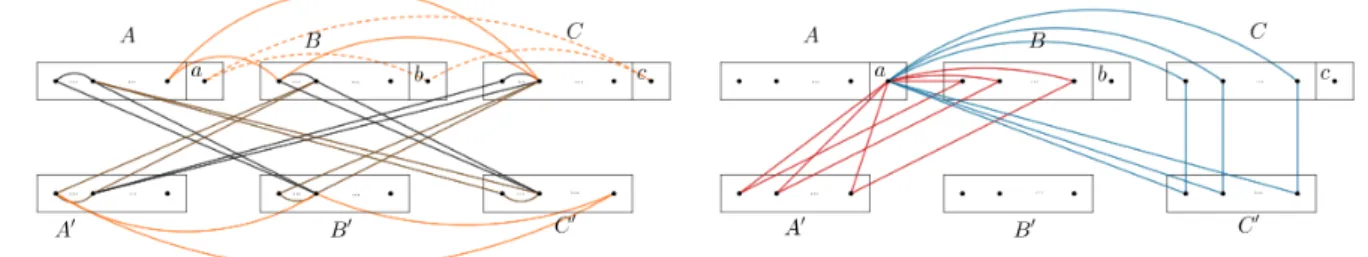
Construction 3.5. The vertex set of F is the disjoint union of 6 smaller subsets (we refer to them as classes), namely V = A∪B∪C∪A⁰∪B⁰∪C⁰, where |A| = |B| = |C|= p+ 1 and

|A⁰| = |B⁰| = |C⁰| = p. Denote the elements of A with a₀, a₁, . . . , ap−1 and a special vertex a. Similarly B = {b₀, b₁, . . . , bp−1, b} and C = {c₀, c₁, . . . , cp−1, c}. For A⁰, B⁰, C⁰ we note the corresponding vertices by α, β, γ respectively, and index their elements again from 0 up to p−1.

The set of triples in F are defined as follows:

• black triples:

– between A and B⁰: {a, a_j, βj} (for 0 ≤ j ≤ p−1); and {a_i, a_{2j−i (modp)}, βj} (for 0≤i6=j ≤p−1)

– between B and C⁰: {b, b_j, γ_j} (for 0 ≤ j ≤ p−1); and {b_i, b_{2j−i (modp)}, γ_j} (for 0≤i6=j ≤p−1)

– between C and A⁰: {c, c_j, α_j} (for 0 ≤ j ≤ p −1); and {c_i, c_{2j−i (modp)}, α_j} (for 0≤i6=j ≤p−1)

• brown triples:

– betweenA⁰ andB: {α_i, α_{2j−i (modp)}, b_j} (for 0≤i6=j≤p−1) – betweenB⁰ and C: {β_i, β_{2j−i (modp)}, c_j} (for 0≤i6=j ≤p−1) – betweenC⁰ and A: {γ_i, γ_{2j−i (modp)}, a_j} (for 0≤i6=j ≤p−1)

• orange triples:

– betweenA\ {a}, B\ {b} andC\ {c}: {a_i, b_j, c_{i+j (modp)}} (for0≤i, j≤p−1) – betweenA⁰,B⁰ andC⁰: {α_i, β_j, γ_{i+j+1 (modp)}} (for 0≤i, j≤p−1)

– {a, b, c}

• red triples:

{a, α_j, bj}, {b, β_j, cj} and {c, γ_j, aj} (for0≤j ≤p−1)

• blue triples:

{a, γ_j, cj}, {b, α_j, aj} and{c, β_j, bj} (for0≤j ≤p−1)

Proposition 3.6. The triple system F defined above has the spreading property.

(a) Black, brown and orange triples and{a, b, c} (b) Red and blue triples througha

Figure 1: Overview of the triple types in Construction 3.5

The proof requires some case analysis. The main goal is to show that cl(V⁰) 6= V⁰ ⊂ V(F) for nontrivial subsets. Our tool is the Cauchy–Davenport theorem (see Theorem 2.1), which simplifies the analysis to those cases where apart from the special verticesa, b, c, we have |V⁰∩ (A∪B∪C)| ≤3 and|V⁰∩(A⁰∪B⁰∪C⁰)| ≤3. For the sake of completeness the proof is carried out in the Appendix.

We continue with a construction which shows a linear upper bound on the minimum size of weakly spreading systems. This will be derived from the upper bound of Theorem 1.10 and completes the proof of the upper bound of Theorem 1.11.

Construction 3.7(Crowning construction). Consider a linear spreading systemF onnvertices andξ_sp(n) = ¹₃ ⁿ₂

−Cn²

triples, with the appropriate constant C. Assign a new vertexv(xy) to every not-covered edge xy of the underlying graph G= G(F), and add newly formed triples by taking {{x, y, v(xy)}:xy6∈G}.

Proposition 3.8. Construction 3.7 provides a weakly spreading system onn+Cn² vertices with

1 3

n 2

+ 2Cn²

triples, hence we obtain

ξ_wsp(N)≤ 2

3N+ 1 6CN.

The deletion of an arbitrary subset of the new vertices of form v(xy) provides also a weakly spreading system.

Proof. It is easy to verify that any two triples, whose underlying set is denoted byV⁰, determine at least three vertices which are not newly added such that they do not form a triple inF. By the spreading property of F, we get that cl(V⁰) contains all points besides the new ones. Through the newly formed triples we get that actually every vertex is contained in cl(V⁰).

Proof of Theorem 1.11, upper bound. Let us choose the smallest odd primepsuch that the sum of the number of vertices and uncovered edges in Construction 3.5 is at least N. Consider Construction 3.7 built on this spreading system and delete a subset of new vertices to obtain a triple system onnvertices. The bound thus follows from the application of Proposition 3.8 with C = ₁₂¹, if we take into account the result on the gaps between consecutive primes [3], similarly to Corollary 1.9.

4 Related results and open problems

In this section we point out several related areas. First we discuss the connection to the topic of Latin squares, a message of which is that similar structures often provide constructions for the problem in view.

4.1 Latin squares

A Latin square of ordernis ann×nmatrix in which each one ofnsymbols appears exactly once in every row and in every column. A subsquare of a Latin square is a submatrix of the Latin square which is itself a Latin square. Note that Latin squares of order nand 1-factorizations of complete bipartite graphsK_n,n are corresponding objects. We will apply the following theorem due to Maenhaut, Wanless and Webb [20], who were building on the work of Andersen and Mendelsohn [2].

Theorem 4.1 (Maenhaut, Wanless and Webb, [20]). Subsquare-free Latin squares exists for every odd order.

Note that for prime order the statement follows from the Cauchy–Davenport theorem, since the Cayley-table of group of prime order gives an instance. The construction presented below not only gives a simple weakly spreading construction, but it may provide an ingredient to a possible extension of Construction 3.5, where the triangle decomposition of the balanced complete tripartite graph, denoted by the set of orange triples, were obtained by a Cauchy–Davenport argument in the prime order case.

Construction 4.2. Take a subsquare-free Latin square of odd order n with row set U, column set V and symbol set W. We assign a triple system T on U ∪V ∪W to the Latin square as follows. Let T = {u_i, v_j, w_k} ∈ T if and only if w_k is the symbol in position (i, j) in the Latin square.

Proposition 4.3. Construction 4.2 yields that the minimum size of a weakly spreading triple system is at mostξwsp(n)≤ ⁿ₉² for n≡3 (mod 6).

Proof. Observe first that every pair of elements from different classes is contained exactly once in the system T. Thus we have to show that there does not exist a subsystem of T spanned by U⁰ ⊆ U, V⁰ ⊆ V and W⁰ ⊆ W for which every pair or elements from different classes is contained exactly once in a triple of the subsystem. Clearly the existence would only be possible if 1 < |U⁰|= |V⁰| =|W⁰| < n but such a system would be equivalent to a Latin subsquare, a contradiction.

4.2 Influence maximization

A social network represented by the graph of relationships and interactions in a group of indi- viduals plays a fundamental role as a medium for the spread of information, ideas, and influence among its members. Models for the processes where some sort of influence or information prop- agate through a social network have been studied in a number of domains, including sociology, psychology, economics and computer science. The influence of a set of nodes is the (expected) number of active nodes at the end of the propagation process in the model and the influence maximization question asks for the set of given size which has the largest influence. In one of the models, called the threshold model (cf. [6]) there exists a threshold value t(v) for every vertex

v∈V and in each discrete step a vertex is activated if it has at leastt(v)active neighbours. For more details we refer to the recent surveys [4, 14] and to the pioneer papers of Domingos and Richardson [9] and Kempe et. al. [18].

Mostly in models of social networks one only considers the graph of relationships, however in applications the propagation may depend more on whether an individual is influenced by the majority of the group members of social groups he or she belongs to. In that context, one has to describe the groups as hyperedges of a hypergraph, and in case of linear3-graphs, the propagation of a vertex set V would clearly influence its closure cl(V). Hence our results determine bounds on the number of3-sets needed so that every set of 3 vertices besides the triples themselves, or every pair of triples has maximum influence.

4.3 Connectivity, backward and forward 3-graphs

First we recall the concept of k-vertex-connectivity of hypergraphs (cf. [12]), which is strongly related to the properties in view, and introduce a new edge-connectivity concept for triple sys- tems.

Definition 4.4. A hypergraph F is k-vertex connected if |V(F)| ≥ k and there is no set W ⊂ V(F) of size at most k−1 such that its removal disconnects F. F is disconnected if there exist a vertex partition {U, V \U} such that the triples of F are spanned by either U or V \U.

A 3-uniform hypergraph F is strongly connected if every vertex partition {U, V \U} induces a triple T with |T ∩U|= 2, provided |U| ≥4.

The latter definition implies that if the partition classes U and V \U are large enough, then triples of type|T ∩U|= 2and |T ∩U|= 1both should appear. The condition|U| ≥4 enables us to apply this concept for linear 3-graphs. We note that the spreading property is stronger than the strong connectivity, while the weakly spreading property is weaker.

Observation 4.5. A Steiner triple system is subsystem-free, that is, spreading if and only if it is strongly connected. Every spreading linear triple system is strongly connected. Every strongly connected3-graph is weakly spreading.

Finally, we underline that the weakly spreading property is not a local one, as the condition cl(V⁰) ⊃ V⁰ restricted to every pair of triples, V⁰ =V(F⁰) with |F⁰| = 2 by no means implies weakly spreading. This follows from the construction below.

Construction 4.6. Consider the complete graph Kn on nvertices n >3, and add a vertex vij

to every graph edge v_iv_j. The obtained triple systemF_(n) ={{v_i, v_j, v_ij}|i6=j≤n} on ⁿ₂ +n vertices with ⁿ₂

hyperedges has the property that every pair of triples generate at least one further triple, but their closure will correspond to either F₍₃₎ or F₍₄₎.

We finish this subsection by mentioning a connection to directed hypergraphs. A directed hyper- edge is an ordered pair,E= (X, Y), of disjoint subsets of vertices whereX is the tail whileY is the head of the hyperedge. Backward, resp. forward 3-graphs are defined as directed3-uniform hypergraphs with hyperedges having a singleton head, resp. tail, see e.g. [16]. These objects have many applications in computer science, operations research, bioinformatics and transport networks.

It is easy to see that if one directs each triple of a linear 3-graph in all possible three ways to obtain a backward edge, then the strong connectivity, described above, of the triple system and the connectivity of the resulting directed hypergraph are equivalent (cf. [16]).

4.4 Further results and open problems

We also mention the recent related work of Nenadov, Sudakov and Wagner [21] on embedding partial Steiner triple system to a small completeSTS, and in general, embedding certain partial substructures to complete structures. In the spreading problem of linear 3-graphs, one may consider the triples of the hypergraph as a collinearity prescription for triples of points. Under this condition the aim would be to describe those affine or projective planes of given order q in which the prescription can be fulfilled, i.e. the corresponding partial linear space can be embedded into the geometry in view. This is closely related to the problem of embedding partial geometries to a given geometry but we allow collinearity prescriptions for triples concerning the same line.

While our Theorem 1.8 on the expander property was sharp, our results Theorem 1.10 and 1.11 concerning spreading and weakly spreading determined the corresponding parameter only up to a small constant factor. The authors believe that if n is large enough, then neither of the bounds are sharp; however it seems a hard problem to asymptotically determine the exact values, similarly to many other extremal problems in hypergraph theory. We finish our paper with several open problems.

Problem 4.7. Is the asymptotically best upper bound on the minimum size ξ_wsp(n) of a lin- ear weakly spreading triple system obtained by the Crowning Construction 3.7 from an optimal construction for ξsp(n)?

Although the lower boundξ_wsp(n) is tight forn≤10, we conjecture that this might be the case, meaning that(C+o(1))n≤ξ_wsp(n) for some C >1.

Problem 4.8. Generalize the results to r-uniform (linear) hypergraphs F.

In order to do this, one should define the neighbourhood and closure accordingly: a vertex z in the neighbourhood of V⁰, if and only if there exist a hyperedgeF ∈ F containingz such that

• either|F∩V⁰| ≥ ^r₂ (majority rule)

• or |F ∩V⁰| ≥t,t < r fixed (large intersection).

Problem 4.9. Prove the existence of a Steiner triple system STS(n) of arbitrary admissible order n, for which

|N(V⁰)| ≥ |V⁰| −3 for every V⁰ ⊂V(G) of size|V⁰| ≤ ^|V₂^|.

AcknowledgementThe authors are grateful to Kristóf Bérczi for his comments and for pointing out several related areas. We also gratefully thank the anonymous referees for their useful suggestions.

References

[1] Alon, N., Boppana, R., Spencer, J. (1998). An asymptotic isoperimetric inequality, Geom.

and Funct. Anal., 8, 411–436.

[2] Andersen, L. D., Mendelsohn, E. (1982). A direct construction for Latin squares with- out proper subsquares. In North-Holland Mathematics Studies (Vol.65, pp. 27–53). North- Holland.

[3] Baker, R. C., Harman, G., Pintz, J. (2001). The difference between consecutive primes, II.

Proceedings of the London Mathematical Society, 83(3), 532–562.

[4] Banerjee, S., Jenamani, M., Pratihar, D. K. (2018). A Survey on Influence Maximization in a Social Network. arXiv preprint arXiv:1808.05502.

[5] Bohman, T., Warnke, L. (2018). Large girth approximate Steiner triple systems. Manuscript, arXiv:1808.01065.

[6] Chen, N. (2009). On the approximability of influence in social networks. SIAM J. Discrete Mathematics, 23(3), 1400–1415.

[7] Conlon, D. (2019). Hypergraph expanders from Cayley graphs. Israel J. Math. 233, 49–65.

[8] Conlon, D., Tidor, J., Zhao, Y. (2018). Hypergraph expanders of all uniformities from Cayley graphs. arXiv preprint arXiv:1809.06342.

[9] Domingos, P., Richardson, M. (2001). Mining the network value of customers. In Proceedings of the seventh ACM SIGKDD international conference on Knowledge discovery and data mining (pp. 57–66). ACM.

[10] Doyen, J. (1969). Sur la structure de certains systemes triples de Steiner. Mathematische Zeitschrift, 111(4), 289–300.

[11] Doyen, J. (1970). Systèmes triples de Steiner non engendrés par tous leurs triangles. Math- ematische Zeitschrift, 118(3), 197–206.

[12] Drewes, F. (1993). Recognising k-connected hypergraphs in cubic time. Theoretical Com- puter Science, 109(1-2), 83–122.

[13] Erdős, P. (1973). Problems and results in combinatorial analysis. In Colloq. Internat. Theor.

Combin. Rome 3–17.

[14] Li, Y., Fan, J., Wang, Y., Tan, K. L. (2018). Influence maximization on social graphs: A survey. IEEE Transactions on Knowledge and Data Engineering, 30(10), 1852–1872.

[15] Fox, J., Gromov, M., Lafforgue, V., Naor, A., Pach, J. (2011). Overlap properties of geo- metric expanders. In Proceedings of the twenty-second annual ACM-SIAM symposium on Discrete algorithms (pp. 1188–1197). Society for Industrial and Applied Mathematics.

[16] Gallo, G., Longo, G., Pallottino, S., Nguyen, S. (1993). Directed hypergraphs and applica- tions. Discrete applied mathematics, 42(2-3), 177–201.

[17] Glock, S., Kühn, D., Lo, A., Osthus, D. (2018). On a conjecture of Erdős on locally sparse Steiner triple systems. arXiv preprint arXiv:1802.04227.

[18] Kempe, D., Kleinberg, J., Tardos, É. (2003). Maximizing the spread of influence through a social network. In Proceedings of the ninth ACM SIGKDD international conference on Knowledge discovery and data mining (pp. 137–146).

[19] Kirkman, T.P. (1847). On a problem in combinatorics, Cambridge Dublin Math. J. 2, 191–

204.

[20] Maenhaut, B., Wanless, I. M., Webb, B. S. (2007). Subsquare-free Latin squares of odd order. European Journal of Combinatorics, 28(1), 322–336.

[21] Nenadov, R., Sudakov, B., Wagner, A. Z. (2019). Completion and deficiency problems. arXiv preprint arXiv:1904.01394.

[22] Stinson, D. R. (2007). Combinatorial designs: constructions and analysis. Springer Science

& Business Media.

[23] Tao, T., Vu, V. H. (2006). Additive combinatorics (Vol. 105). Cambridge University Press.

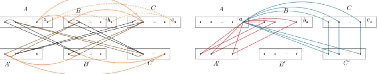
5 Appendix – Proof of Theorem 3.6

Here we prove that Construction 3.5 has the spreading property, i.e. cl(V⁰) =V for all nontrivial sets V⁰. Note that the construction corresponds to a triangle decomposition of a graphGwhich is a perturbation of K6p\(Kp,p∪K˙ _p,p∪K˙ _p,p).

The first step is to verify the statement for those setsV⁰ which have a large enough intersection with eitherA∪B∪C or A⁰∪B⁰∪C⁰, by the application of the Cauchy–Davenport theorem.

(a) Black, brown and orange triples and{a, b, c} (b) Red and blue triples througha

Figure 2: Overview of the triple types in Construction 3.5

Observation 5.1. Let us denote the set (A\ {a})∪(B\ {b})∪(C\ {c}) by U. If|V⁰∩U|>3 or |V⁰∩(A⁰∪B⁰∪C⁰)|>3, and V⁰ intersects with at least two different classes thencl(V⁰) =V. Indeed, without loss of generality, suppose to the contrary that there exists a set |V⁰ ∩(A⁰∪ B⁰∪C⁰)|>3 withA₀ =V⁰∩A⁰, B₀ =V⁰∩B⁰, C₀ =V⁰∩C⁰ from whichC₀ has the least size (smaller than p), such thatcl(V⁰) =V⁰. Apply the Cauchy–Davenport theorem (Theorem 2.1) for A0 and B0 to obtain |A₀ +B0| ≥ min{|A₀|+|B₀| −1, p} > |C₀|. Thus the orange triples with their additive structure ensure that|cl(V⁰)∩C⁰|>|C₀|, a contradiction.

In the rest of the proof we point out that no matter how we choose a nontrivial set V⁰ of 3 elements{x, y, z}, its closure contains at least4elements from either U or A⁰∪B⁰∪C⁰, coming from more than one class, thus the application of Observation 5.1 in turn completes the proof.

1. {x, y, z} ⊂A∪B∪C:

a) |{x, y, z} ∩ {a, b, c}|= 0:

a1) If the starting elements are not in the same class (A,B or C) then two of them from different classes determine a new element (moreover it cannot be the special vertex) from the third class via an orange triple and now we have 4 elements of the closure inU not from the same class.

a2) WLOG we can assume that x=ai, y =aj, z=a_k fromA\ {a}. By using black and brown triples a_i, a_j determine some β_l; a_i, a_k determine some β_m (m 6= l) andβl, βm determine some cs∈C\ {c}.

b) |{x, y, z} ∩ {a, b, c}|= 1, WLOG let’s assume that z=a:

b1) Ifx, y are in different classes then they determine a new element from the third class via an orange triple thus we have got now 4 elements: a_i, a, b_j, c_k. From a and ck we get γk due to a blue triple. If j 6=k then bj and γk determine some bm through a black triple, and the closure meets U in more than 3 elements. If

j = k then i = 0 must hold, therefore b and β0 are in the closure from black triples formed by{b, b_k, γ_k}and {a, a₀, β₀}. Now bandβ₀ determinec₀ via a red triple, and we are done unless i=j =k = 0. In that case, one can verify that the closure contains{a₀, b0, c0, α0, β0, γ0, a, b, c}and byα0 andβ0 we get thatγ1

is in the closure via an orange triple henceγ₀ andγ₁ determinea^p+1

2

via a brown triple that is the fourth element fromU.

b2) If x, y are in the same class then a, x and a, y determine different elements of the same class from A⁰∪B⁰∪C⁰ therefore these two elements determine a new element ofU hence we trace back to case a).

c) |{x, y, z} ∩ {a, b, c}|= 2, WLOG let’s assume that z=aand y=b:

c1) if x = ci ∈ C\ {c} then a and ci determine γi via a blue triple, then b and γi

determineb_i ∈B\ {b} due to a black triple therefore we trace back to case b1).

c2) if x = b_i ∈B \ {b} then b and b_i determine γ_i via a black triple, then aand γ_i determineci∈C\ {c} therefore we trace back to case b1).

c3) if x = a_i ∈ A\ {a} then b and a_i determine α_i via a blue triple, then aand α_i determineb_i ∈B\ {b} due to a red triple therefore we trace back to case b1).

2. {x, y, z} ⊂A⁰∪B⁰∪C⁰:

One can deduce that this case can be discussed precisely the same way as case 1.a).

3. |{x, y, z} ∩(A∪B∪C)|= 2:

Assume that{y, z} ⊂A∪B∪C and x∈A⁰∪B⁰∪C⁰. a) |{y, z} ∩ {a, b, c}|= 0:

a1) Ifyandzare not in the same class then they determine a new non-special element from the third class through an orange triple. Together with the element from A⁰ ∪B⁰∪C⁰ one of these elements will form a triple which gives another new element fromA∪B∪C. Either the closure meetsU in more than 3 elements or trace back to case 1.b).

a2) WLOG we can assume that z = ai and y =aj. These two elements determine some β_k due to a black triple. Now if x =β_l then from β_k and β_l we can get a c_m due to a brown triple and then apply 1.a1). Ifx=γ_l then at least one of the pairs γl, ai or γl, aj can determine a new element γm via a brown triple and we get a situation like in case 2. Ifx =α_l then α_l,β_k determine some γ_m through an orange triple and we get back the previous case.

b) |{y, z} ∩ {a, b, c}| 6= 0:

WLOG suppose thatz=a. Now atogether with the element fromA⁰∪B⁰∪C⁰ will determine a new element fromU hence we trace back to case 1.b) or 1.c).

4. |{x, y, z} ∩(A∪B∪C)|= 1:

a) If the two elements fromA⁰∪B⁰∪C⁰ are in different classes then via an orange triple they determine a new element from the third class and together with the element from A∪B∪C they can determine at least one new element which is either inA⁰∪B⁰∪C⁰ and we are done or from A∪B∪C thus trace back to case 3.

b) If the two elements fromA⁰∪B⁰∪C⁰ are in the same class then they determine a new element fromU and we trace back to case 3.