Multi-Project Optimization with Multi-Functional Resources by a Genetic Scheduling Algorithm

Multi-Project Optimization with Multi-

Functional Resources by a Genetic Scheduling Algorithm

Tibor Dulai, György Dósa, Ágnes Werner-Stark

University of Pannonia, Egyetem u. 10, H-8200 Veszprém, Hungary dulai.tibor@virt.uni-pannon.hu

dosagy@almos.uni-pannon.hu werner.agnes@virt.uni-pannon.hu

Abstract: In this paper we show how a genetic scheduler algorithm can be applied to solve a hard multi-project optimization problem with shared resources. The resources work in multiple operation modes, so they can substitute each other (but with different efficiency).

We consider processes which have quite complex structure, i.e., it allows the existence of parallel sub-processes. This problem is extremely complex, there is no chance to get the optimal solution in reasonable time. The proposed algorithm intends to find a near-optimal solution, where the goal of the optimization is the minimization of the makespan of the schedule. We present the genetic operations of the algorithm in detail. We fill the pool of populations only with feasible solutions, but making possible the discovery of the whole search space. The feasibility of a schedule is ensured by excluding time-loops regarding the sequence of the tasks both in their process and in the queue of their resource. We executed several tests for determining the (hopefully) optimal parameters of the algorithm regarding the number of generations, the population size, the crossover rate and rate of the mutation.

We applied the algorithm for many problem classes where the parameters of the input are fixed or randomly chosen from some interval.

Keywords: multi-project scheduling; genetic algorithm; multi-purpose machines

1 Introduction

Scheduling is a widespread research area of operations research. The classes of the problem differs, e.g. in the number of the resources (machines) or in the properties of the tasks to schedule. Two important versions of the problem are the flow-shop problem [5, 10] and the job-shop problem. [2, 11]

As the basic scheduling problem ‒ called job-shop scheduling problem (JSP), where a set of jobs have to be scheduled on a set of machines regarding certain criterion(s) ‒ is NP-hard [6], heuristics and more effective meta-heuristics are often used for real-life sized problems instead of exact solution methods. An

effective meta-heuristic is genetic algorithm (GA), in [15] Zhang et al. reviewed some of GA applications for flexible JSP and introduced their own problem representation and genetic operators. It was followed by the presentation of their computational results on common benchmark data sets. Next to GA other heuristics like tabu search [7] or simulated annealing [9] are also popular methods.

The application area of different scheduling problems has a wide spectrum. In computer architecture and parallel software planning tasks have to be scheduled on processors (e.g. on CPU and GPU), in industrial or business applications workflow elements have to be assigned to resources and scheduled in time, while, e.g. in software project scheduling project-tasks have to be scheduled mainly on a human-based resource set usually in a dynamic manner. The different application areas differ in their requirements and have their own specialities.

Nevertheless, the complexity of the basic problem remains, what necessitates the usage of heuristics. Votava [14] simulated two heuristic algorithms (named HEFT and CPOP) for task scheduling in a networking subsystem. Alba and Chicano [1]

shown that GA is an appropriate tool for project scheduling and can be applied efficiently for automated task assignment. Chang et al. [4] - extending their former work [3] - presented a GA with improved representation and parameters, which took into account more human resource factors. Moreover, as the representation introduced a timeline axis as a third dimension (next to tasks and resources), it made possible the suspension and resumption of tasks and the reassignment of resources.

Sadegheih used simulated annealing for determining the effect of GA parameters on the schedule [13]. In his work he dealt with 8-jobs and 7-machines problems and found the importance of mutation rate and not significant effect of crossover rate.

Joo et al. [8] dealt with multi-project scheduling with multimode resources and applied activity splitting and simulated annealing. In this paper, a genetic algorithm for scheduling in multi-project environment is presented, where resources may have multiple functions, so they can substitute each other. The representation of a schedule is shown, the developed crossover and mutation genetic operators are introduced. The algorithm is able to cover the whole feasible search space during its operation. The paper emphasizes the method for guarantying the feasibility of the schedule by eliminating possible time loops what could arise after applying genetic operators.

Pongcharoen et al. [12] dealt with similar sized problem as ours (similar number of resources and tasks), too, however, their problem had not such a complex structure. They investigated population size, generation number, mutation and crossover rates. While determining optimal parameters of GA they also described how they face and eliminate time-loop (they called it deadlock). If they got an infeasible schedule, they swapped the problematic action with a random one. In our paper we handle this problem in other way.

In Section 2 the model of the problem is introduced and described formally.

Section 3 presents the genetic algorithm and its operators we applied. In Section 4 we summarize the computational results, while Section 5 concludes our work.

2 The Example Processes and the Model of the Problem

2.1 The Basic Example Processes

This subsection introduces the problem we worked on, for illustrative purposes. In our simulations we used two kinds of processes: the tested production of 15 pieces of sensor type I and 20 pieces of sensor type II. Altogether, it means that we deal with 35 processes, parallel. The processes of producing one of each types of these products are illustrated in Figure 1.

Figure 1

The two types of our example processes

In the figure we can see the sequence of tasks in processes. Tasks without caption are transportation tasks from one resource to another. The initial and final destination is the depot. The duration time of each task depends on the resource which operates, as Table 1 shows. In the table Tr. marks transportation task, Tr.d.

holds for a transportation device followed by the abbreviated places of work phases (moreover d stands for the depot). In our example all the transportation devices have to get back to their starting place if we want to reuse them, and it takes the same time as to carry the materials to a place of work. For example, a transportation device can transfer a material from the depot to the place of temperature test in 3 time units, however, we have to wait 6 time units if we want to reuse it. The table also contains how many pieces of the different resources are available at all.

In our example we apply setup time only in case of temperature chamber and vibration chamber. If they change their operation mode between temperature test and vibration test, symmetrical setup times are used. For temperature chamber we defined 5 time units as setup time and for the vibration chamber we determined the setup time as 6 time units.

Table 1

Duration time of each task related to its resource usage /in time units/

Tr.

d-t Temp.

test Tr.

t-s

Solde- ring

Tr.

s-d Tr.

d-c Cab- ling

Tr.

c-s Tr.

t-v Vibr.

test Tr.

v-s Temperature

chamber (3 pieces)

- 6 - - - - - - - 10 -

Cable producer (2 pieces)

- - - - - - 6 - - - -

Vibration chamber (1 piece)

- 10 - - - - - - - 6 -

Solderer (2 pieces)

- - - 4 - - - - - - -

Tr.d. d-t (1 piece)

3 - - - - - - - - - -

Tr.d. d-c (1 piece)

- - - - - 5 - - - - -

Tr.d. t-s (1 piece)

- - 4 - - - - - - - -

Tr.d. t-v (1 piece)

- - - - - - - - 3 - -

Tr.d. c-s (1 piece)

- - - - - - - 3 - - -

Tr.d. v-s (1 piece)

- - - - - - - - - - 5

Tr.d. s-d (1 piece)

- - - - 4 - - - - - -

Tr: transport; Tr.d.: transportation device; d: depot; c: cable producing; t: temperature test;

v: vibration test; s: soldering

An example for a schedule can be seen in Figure 2 for a scenario where 3 processes exist: 2 of them test and produce sensor type I and 1 of them tests and produces sensor type II. In the figure (Figure 2) each rectangle of a task contains its process ID. Moreover, empty boxes represent the duration while a transportation device reaches back to its start place.

Figure 2

A simple schedule as a result of our algorithm

Several similar problems − with the same process structure, conditions and constraints − can be found in real-life practice (e.g. producing and packing a

porcelain in a manufacture requires parallel execution of tasks packaging material preparation and creation of the porcelain). There can be orders that require pure sculpted porcelain, while other orders necessitate paint. Human resources of the manufacture are specialized: there are potters and painters. Painters are better (and quicker) in paint and potters are better in sculpting. However, they can execute the task of the other specialists, too, but significantly slower. When both the porcelain and the packaging material are ready, the porcelain has to be packaged by a third type of specialist of the company.

Next to this second example, other industrial/business processes may have the same characteristics.

2.2 Difficulties of the Problem

The complexity of the algorithm showed in this paper origins from the properties of the problem that we intend to solve. The problem class is a scheduling problem where resources have to be allocated to carry out the tasks of a process and the allocations have to be ordered in the time domain. However, as common practical scheduling problems, the basic problem has some other properties:

• we deal with multiple processes parallel, which may share in the resources they use,

• each process can include parallel substructure(s) of tasks instead of a fully sequential order of its ingredient tasks,

• resources can operate in different operation modes. There are tasks, which can be carried out by more than one resources (usually with different parameters like operation time), and there are resources, which are able to do different tasks. It results in resource-substitution possibilities.

These properties make the problem extremely complex, e.g. related to the common NP-hard P_m||C_max problems.

2.3 Notations

The input is given as follows:

• P = {p₁, ..., p_n} is the set of processes.

• T_i = {t_i,1, ..., t_i,m} is the set of tasks of process p_i.

• T = ᴗⁿi=1T_i is the set of the tasks of all processes.

• Pre(t_i,j) С Ti is the subset of the tasks of process p_i (what can be an empty set) which are direct prior tasks to task t_i,j in process p_i. This set may have

more than one element because of the possible parallel structure of processes.

• allPre(t_i,j) С Ti is the subset of the tasks of process p_i (what can be an empty set) which are prior tasks to task t_i,j in process p_i. E.g. if t_i,b є Pre(t_i,c) and t_i,aє Pre(ti,b) then t_i,aє allPre(ti,c).

• R = {r₁, ..., r_o} is the set of resources.

• capable: R x T → {0,1} is a function which describes whether a resource is able to carry out a task.

• dur(t_i,j,r_k) є Nshows the duration time of carrying out task t_i,j by resource r_k, where capable(r_k,t_i,j) = 1.

The schedule-related variables are:

• allocatedRes(t_i,j) є R is the resource which is assigned by the scheduler to task t_i,j.

• start(t_i,j) є N is the start time of task t_i,j of process p_i.

• end(t_i,j) є N is the end time of task t_i,j of process p_i.

• makespan(P) = max(end(t_i,j)) - min(start(t_k,l)) for all t_i,j, t_k,lє T.

2.4 Constraints

The constraints for determining start(ti,j) and end(ti,j) for all ti,j є T are:

𝑎𝑎𝑎𝑎𝑎𝑎𝑎𝑎𝑎𝑎𝑎𝑎𝑎𝑎𝑎𝑎𝑎𝑎𝑎𝑎𝑎𝑎𝑎𝑎(𝑎𝑎_{𝑖𝑖,𝑗𝑗})≠ ∅,∀𝑎𝑎_{𝑖𝑖,𝑗𝑗}∈ 𝑇𝑇 (2.1)

So, each task has to be carried out by a resource.

𝑎𝑎𝑒𝑒𝑎𝑎(𝑎𝑎_{𝑖𝑖,𝑗𝑗}) = 𝑎𝑎𝑎𝑎𝑎𝑎𝑠𝑠𝑎𝑎(𝑎𝑎_{𝑖𝑖,𝑗𝑗}) +𝑎𝑎𝑑𝑑𝑠𝑠(𝑎𝑎_{𝑖𝑖,𝑗𝑗},𝑎𝑎𝑎𝑎𝑎𝑎𝑎𝑎𝑎𝑎𝑎𝑎𝑎𝑎𝑎𝑎𝑎𝑎𝑎𝑎𝑎𝑎𝑎𝑎(𝑎𝑎_{𝑖𝑖,𝑗𝑗})),∀𝑎𝑎_{𝑖𝑖,𝑗𝑗}∈ 𝑇𝑇 (2.2) The above constraint represents the connection between the start and finish time of a task regarding the related operation time.

𝑎𝑎𝑎𝑎𝑎𝑎𝑠𝑠𝑎𝑎�𝑎𝑎_{𝑙𝑙,𝑚𝑚}� ≥ 𝑎𝑎𝑒𝑒𝑎𝑎�𝑎𝑎_{𝑖𝑖,𝑗𝑗}�𝑎𝑎𝑠𝑠 𝑎𝑎𝑒𝑒𝑎𝑎�𝑎𝑎_{𝑙𝑙,𝑚𝑚}� ≤ 𝑎𝑎𝑎𝑎𝑎𝑎𝑠𝑠𝑎𝑎�𝑎𝑎_{𝑖𝑖,𝑗𝑗}�,∀𝑎𝑎_{𝑖𝑖,𝑗𝑗},𝑎𝑎_{𝑙𝑙,𝑚𝑚}∈ 𝑇𝑇,𝑖𝑖𝑖𝑖 𝑎𝑎_{𝑖𝑖,𝑗𝑗}≠

𝑎𝑎𝑙𝑙,𝑚𝑚 𝑎𝑎𝑒𝑒𝑎𝑎 𝑎𝑎𝑎𝑎𝑎𝑎𝑎𝑎𝑎𝑎𝑎𝑎𝑎𝑎𝑎𝑎𝑎𝑎𝑎𝑎𝑎𝑎𝑎𝑎�𝑎𝑎𝑖𝑖,𝑗𝑗� ≡ 𝑎𝑎𝑎𝑎𝑎𝑎𝑎𝑎𝑎𝑎𝑎𝑎𝑎𝑎𝑎𝑎𝑎𝑎𝑎𝑎𝑎𝑎𝑎𝑎�𝑎𝑎𝑙𝑙,𝑚𝑚� (2.3)

This constraint specifies that the tasks allocated to the same resource can not overlap each other.

𝑎𝑎𝑒𝑒𝑎𝑎(𝑎𝑎_{𝑖𝑖,𝑎𝑎})≤ 𝑎𝑎𝑎𝑎𝑎𝑎𝑠𝑠𝑎𝑎(𝑎𝑎_{𝑖𝑖,𝑏𝑏}),∀1≤ 𝑖𝑖 ≤ 𝑒𝑒,∀𝑎𝑎_{𝑖𝑖,𝑎𝑎},𝑎𝑎_{𝑖𝑖,𝑏𝑏}∈ 𝑇𝑇_𝑖𝑖,𝑖𝑖𝑖𝑖 𝑎𝑎_{𝑖𝑖,𝑎𝑎}∈ 𝑎𝑎𝑎𝑎𝑎𝑎𝑎𝑎𝑠𝑠𝑎𝑎(𝑎𝑎_{𝑖𝑖,𝑏𝑏}) (2.4) The final constraint describes that a task of a process can not start before its prior tasks of the same process are not finished.

We look for a schedule where all constraints 2.1-2.4 are satisfied and the makespan(P) is minimal.

3 The Genetic Algorithm

The scheduling of real workflows − especially in multi-project environment − requires more and more computational power regarding the increasing of the number and complexity of the processes. It is the reason for preferring heuristics to exact solvers for solving them. This paper presents a genetic algorithm which was developed for scheduling workflows/processes even if they have the properties introduced in Section 2.

Genetic Scheduler (GS):

The GS has the following steps:

Step 1. An initial population is filled up by random instances.

Step 2. Evaluation of the instances of the initial population (a fitness value is calculated for each of the instances of the population).

Step 3. Applying elitism the best x percent of the generation is copied into the new generation.

Step 4. The remaining instances of the new generation are selected and copied randomly from the previous generation.

Step 5. We apply crossover genetic operator to the new generation: a randomly selected instance of the new generation will be replaced by the resulted child instance.

Step 6. We apply mutation genetic operator to the instances of the new generation.

Step 7. Fitness value is calculated for each of the instances of the new generation.

Step 8. While the desired generation number is not reached: GOTO Step 3.

The details of the algorithm are presented in the following subsections.

3.1 Representation

The genetic algorithm requires a solution − a schedule − to be represented by a coding technique that results a coded instance, on what, it is easy to apply the genetic operators and what is unambiguous. Since an instance is unambiguously described by the resource-assignment and the sequence of the tasks at each of the resources − what clearly defines the timing of the task as we intend to minimize the makespan so start each task as soon as possible −, it is enough only to store these data as an instance representation. We chose a two dimensional data structure (PS) for this type of representation: the first dimension represents the resources while the second dimension shows the sequenced tasks assigned to the resources.

PS is a pseudo-instance of a schedule, where

𝑎𝑎𝑃𝑃𝑖𝑖𝐶𝐶 𝑇𝑇 𝑎𝑎𝑒𝑒𝑎𝑎 𝑎𝑎𝑎𝑎𝑎𝑎𝑎𝑎𝑎𝑎𝑎𝑎𝑎𝑎𝑎𝑎𝑎𝑎𝑎𝑎𝑎𝑎𝑎𝑎�𝑎𝑎𝑘𝑘,𝑙𝑙�=𝑠𝑠𝑖𝑖 ∀𝑎𝑎𝑘𝑘,𝑙𝑙∈ 𝑎𝑎𝑃𝑃𝑖𝑖,∀1≤ 𝑖𝑖 ≤ 𝑎𝑎 𝑎𝑎𝑒𝑒𝑎𝑎 𝑎𝑎𝑃𝑃𝑖𝑖≠ 𝑎𝑎𝑃𝑃𝑗𝑗 𝑖𝑖𝑖𝑖 𝑖𝑖 ≠ 𝑗𝑗,

moreover PSi,jє T means that this task is assigned to resource ri and is the j^th ordered element among the tasks assigned to ri.

Figure 3

The representation of an instance

Figure 3 illustrates a simple instance as an example for the coding we apply. As we have introduced, t_i,j signs the j^th task of the i^th process. For the sake of perspicuity, we used for the illustration of the tasks which belong to the same process the same color. As the coding schema shows, the representation includes only sequences, it has not exact timing data neither task duration.

3.2 Population

We create the initial population of the genetic algorithm populated by instances presented in subsection 3.1. The cardinality of the population is determined by an a priori set variable (populationSize).

All of the instances are created as follows:

Step 1. Select randomly one of the unscheduled processes until there exist at least one of them.

Step 2. For each task of the selected process, starting from the first one taking into account the sequence of the tasks, do the followings:

Step 2.1. Collect all the resource which are capable to carry out the task.

Step 2.2. Select randomly one of these resources.

Step 2.3. Select a random feasible position between the ordered tasks of the selected resource.

Step 2.4. Place the task at the selected position (update the instance.) Step 3. GOTO Step 1.

The result of the algorithm is an instance. The number of the instances to create is shown by the population size parameter of the genetic algorithm.

However, step 2.3 is critical: the generated instance has to be feasible. By selecting a nonlegal position for the task to insert a time-loop may evolve. It can happen in two ways:

A In the ordered sequence of the tasks of a resource a later task of a process has the position with a smaller index than an earlier task of the same process. A simple example for it can be seen in Figure 4.

Figure 4

Time-loop related to one resource

B Time-loops may occur involving more than one resource, too. Figure 5 illustrates this kind of time-loop related to two resources, however, the number of the affected resources and tasks can be higher. Since, on one hand task t_2,1 is executed by resource r_x later than task t_1,3, on the other hand task t_2,2 - what has to be executed after task t_2,1of the second process had been finished - is carried out earlier by resource r_y than task t_1,2. Although task t_1,3 should have been processed after task t_1,2 regarding the sequence of the tasks of the first process. If the insertion of a task triggers a situation similar to this, a time-loop occurs.

Figure 5

Time-loop related to one process

After the creation of the initial generation whose population is filled up by random, feasible instances, further generations are generated by using genetic operators on the actual generation. The number of generations is also given by the preset value of a variable.

3.3 Fitness Function

For being able to decide which instances are better, we have to qualify them by a numeric value. In our case the fitness value of an instance is the makespan. It shows how does it take to do all the tasks of the schedule, starting from the beginning of the earliest task until the finishing of the latest one. In this work we deal only with time aspects, however, other parameters also can be involved into the creation of the fitness functions, e.g. the cost of the applied resources, creating a multi-objective problem. For calculating the fitness value of an instance it is important to know that the instance describes the order of the tasks for each resource. This sequence and the knowledge about process-related constraints and the operation times, determine the optimal timing unambiguously. We have to

know the start and finish time of all the tasks for calculating the makespan − the fitness value of a schedule.

For timing three basic ideas have to be followed:

• Each task as to be started as early as possible.

• A task cannot be started until its direct prior task in the queue of the resource is not finished and the resource has not been transferred to the state in which it is ready for doing the new task (the latter duration is called setup time).

• A task can not be started until all of its prior tasks in its process have not been finished.

Keeping these constraints − which result a greedy scheduling − all the tasks are timed. After that the makespan can be calculated, obtaining the fitness value of the instance.

3.4 Elitism

The use of elitism on a generation of the genetic algorithm depends on a parameter of our algorithm, see subsection 3.7. When elitism is applied, then the best instances − instances with the lowest makespan − of the previous generation are copied to the next generation. The quantity of the instances which are handled as elites are set by a parameter of the algorithm. As the cardinality of a generation is unchanged, the remaining part of the new generation has to be filled up by random instances of the previous generation. In our case, other parameter signs whether any member − also the elites − can be selected during this random fill up without return.

3.5 Crossover

After the initial instances of the new generation are determined, our algorithm applies crossover genetic operation on the instances with a priori set probability. If crossover is applied, another parameter shows how percent of the population is created by crossover. Supposing that the value of this parameter is c, the following steps are iterated c times:

Step 1. Select two different instances randomly from the new generation (parent1 and parent2)

Step 2. There is a parameter of the algorithm which shows what percent of the processes are inherited from parent1 and how much from parent2. Based on the value of this parameter:

Step 2.1. Select randomly so many processes from parent1 that it meets the value of the parameter.

Step 2.2. Create a new instance, where the resource assignment for each task of the selected processes is the same as in parent1. The position of the tasks in the row of their resources is random, but taking care of avoiding the creation of time- loops.

Step 2.3. The resource assignment of the tasks of the remaining processes is the same as in parent2. The position of these tasks in the row of their resources is also random, but prevents the creation of time-loops.

The created c pieces of child instances are first put into a temporary storage, then randomly selected instances of the generation is replaced by these children, taking care of not to select an instance which was put into the generation in this phase as a child. There is a parameter of the algorithm that controls whether an elite can be replaced by a child who was created by crossover.

3.6 Mutation

After the possible crossover over the new generation, mutation genetic operator can be applied on the population of the new generation. There is a parameter which shows the probability of whether applying mutation on this generation. If it is applied, another parameter determines the probability of using mutation for each instance of the generation, separately.

Mutating an instance covers the following steps:

Step 1. Select a process randomly from the schedule.

Step 2. Delete all of the tasks of the selected process from the instance.

Step 3. Do the following steps for each task of the process - starting from the first task of the process and processing them in order:

Step 3.1. Collect all the resources which are able to carry out the task.

Step 3.2. Select randomly one from these resources.

Step 3.3. Insert the task into a random, but feasible position of the row of the selected resource.

After all of these operations, the finalized population of the new generation is created. The fitness value of each created instance has to be calculated for qualifying the instances of the new generation and being able to inherit more generations based on the presented rules.

3.7 Parameters of the Algorithm

The developed genetic algorithm has several parameters. These are:

• The size of a population (sizeofPopulation).

• The number of the generations.

• The percent of the instances of a population obtained by elitism (elites).

• When selecting the other (1-elites)*sizeofPopulation instances, whether we can reselect elites, too?

• The possibility for applying crossover on a generation.

• How percent of a generation should be resulted by crossover?

• How percent of the processes origins from the first parent in case of crossover?

• Whether only the instances with the worst fitness values should be replaced by the results of the crossover or any random instances?

• The possibility for applying mutation for a generation.

• The possibility for mutation in case of an instance of a generation which lets mutation to be applied.

• Whether crossover and mutation can influence elites, too?

In our work the execution of the algorithm always happens as long as the parameter of the generation number indicates and does not stop even if it realizes convergence of the results before the preset generation number is reached.

4 Results

The presented algorithm was applied for two kinds of problems. Both of them were based on the problem presented in subsection 2.1, but differ in the definiteness of the process number and the operation time. The first problem realizes exactly the same problem as subsection 2.1 presents. The second one applies stochastic operation time and process number.

4.1 Results for the Deterministic Problem

First, we run several times the algorithm for exactly the same problem presented in subsection 2.1 (with 35 processes) with the following parameter settings:

• sizeofPopulation: 60.

• The number of the generations: 400.

• elites: 0.2.

• When selecting the other instances, we can reselect elites, too.

• The possibility for applying crossover on a generation: 1.

• The percent of a generation should be resulted by crossover: 0.7.

• The percent of the processes origins from the first parent in case of crossover: 0.5.

• Only the instances with the worst fitness values should be replaced by the results of the crossover.

• The possibility for applying mutation for a generation: 1.

• The possibility for mutation in case of an instance: 0.18.

• Crossover and mutation can not influence elites.

Some of the parameters − e.g. 0.18 mutation rate − were based on the values Pongcharoen et al. [12] found to be optimal.

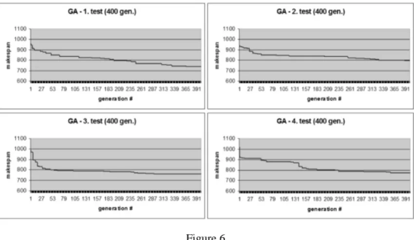
Figure 6 shows that even in case of 400 generation the results (the best makespan) differ significantly.

Figure 6

Some results in case of the deterministic problem, applying GA with 400 generation and 60 population size

After we found this fact, we intended to analyze the effect of the other important parameters both on the makespan of the resulted solution and the convergence of the results we obtained.

In the next step, we changed the value of the population size while all the other parameters of the genetic algorithm stayed unchanged. The results are illustrated in Table 2.

Table 2

Makespan results for the genetic scheduler with variable population size /in time units/

generation: 400, crossover rate: 0.7, mutation rate: 0.18, population size: p p:10 p:20 p:30 p:40 p:50 p:60 p:80 p:100 p:150

Test 1. 857 802 832 802 780 740 770 790 734

Test 2. 854 796 779 796 767 796 743 779 760

Test 3. 834 812 797 844 803 799 775 756 732

Test 4. 876 823 824 792 774 799 761 732 752

Test 5. 829 818 826 804 782 758 808 762 744

The best 829 796 779 792 767 740 743 732 732

Avg. 850 810.2 811.6 807.6 781.2 778.4 771.4 763.8 744.4 Deviation 16.96 9.97 20.26 18.70 12.09 24.69 21.30 19.96 10.61

Table 3

Makespan results for the genetic scheduler with variable crossover rate /in time units/

generation: 400, population size: 100, mutation rate: 0.18, crossover rate: c

c: 0.7 c: 0.5 c: 0.3 c: 0.1

Test 1. 790 708 723 684

Test 2. 779 689 660 710

Test 3. 756 711 683 720

Test 4. 732 708 688 704

Test 5. 762 718 684 700

The best 732 689 660 684

Avg. 763.8 706.8 687.6 703.6

Deviation 19.96 9.62 20.24 11.89

As it can be seen, the higher the cardinality of the population is the better the results we got for the same generation number, however after population size 100 the best makespan does not improve.

In the followings, we fixed the value of the population size 100 and investigated the effect of smaller crossover rates. We collected the results in Table 3.

The results show that crossover rate 0.3 resulted the best makespan and the best average makespan, too. For our further investigation we fixed crossover rate at value 0.3. At this point, we found the importance of well determined crossover rate, unlike in paper by Pongcharoen et al. [12]. The difference may origin from the difference of the design of the genetic operators. The final important parameter we dealt was the mutation rate. Its effect on the efficiency of the genetic algorithm is illustrated in Table 4.

Table 4

Makespan results for the genetic scheduler with variable mutation rate /in time units/

generation: 400, population size: 100, crossover rate: 0.3, mutation rate: m

m: 0.08 m: 0.18 m: 0.28 m: 0.38 m: 0.48

Test 1. 887 723 692 678 682

Test 2. 751 660 674 648 648

Test 3. 707 683 680 676 692

Test 4. 708 688 736 672 674

Test 5. 698 684 692 661 675

The best 698 660 674 648 648

Avg. 750.2 687.6 694.8 667 674.2

Deviation 70.83 20.24 21.75 11.17 14.59

The results show that a higher mutation rate (0.38) has positive effect on the genetic algorithm. Its reason can be that it makes the algorithm jump out of local

optimum more often, but the construction of the algorithm does not let it to leave a better part of the search space for the worse part of that.

4.2 Results for Stochastic Problem

Based on the parameters we determined in the previous subsection, we applied our genetic algorithm on a problem, where operation time and process number are stochastic. The problem includes the same type of processes presented in subsection 2.1. However, the number of processes was changed as follows: the problem produces x pieces of sensor type I where x є [10,20] and y pieces of sensor type II where y є [15,25]. For different executions we selected x and y from their interval based on uniform distribution.

Moreover, the operation times are also stochastic variables, following uniform distribution from the interval presented in Table 5.

Table 5

Duration time selection interval of each task /in time units/ in case of the stochastic problem Tr.

d-t Temp . test

Tr.

t-s Solde -ring

Tr.

s-d Tr.

d-c Cab - ling

Tr.

c-s Tr.

t-v Vibr.

test Tr.

v-s Temperatur

e chamber

- [4,8] - - - - - - - [8,12

] - Cable

producer

- - - - - - [4,8

]

- - - -

Vibration chamber

- [8,12] - - - - - - - [4,8] -

Solderer - - - [3,5] - - - - - - -

Tr.d. d-t [2,4 ]

- - - - - - - - - -

Tr.d. d-c - - - - - [3,7

]

- - - - -

Tr.d. t-s - - [3,5

]

- - - - - - - -

Tr.d. t-v - - - - - - - - [2,4

]

- -

Tr.d. c-s - - - - - - - [2,4

]

- - -

Tr.d. v-s - - - - - - - - - - [3,7

]

Tr.d. s-d - - - - [3,5

]

- - - - - -

Tr: transport; Tr.d.: transportation device; d: depot; c: cable producing; t: temperature test;

v: vibration test; s: soldering

We applied our genetic algorithm with the following parameter settings:

• sizeofPopulation: 100.

• The number of the generations: 400.

• elites: 0.2.

• When selecting the other instances, we can reselect elites, too.

• The possibility for applying crossover on a generation: 1.

• The percent of a generation should be resulted by crossover: 0.3.

• The percent of the processes origins from the first parent in case of crossover: 0.5.

• Only the instances with the worst fitness values should be replaced by the results of the crossover.

• The possibility for applying mutation for a generation: 1.

• The possibility for mutation in case of an instance: 0.38.

• Crossover and mutation can not influence elites.

For this problem the random selected values of 6 test cases are represented in Table 6 and the results of our algorithm for these cases are shown in Table 7.

Table 6

Random selected process numbers and operation time of the resources (the latter in time units, related to their actions, which are illustrated in Table 5 in case of the 6 presented stochastic examples)

1. test 2. test 3. test 4. test 5. test 6. test

sensor type I (pieces) 17 16 13 14 13 18

sensor type II (pieces) 17 23 21 22 15 21

Temperature chamber (temp./vibr. test)

8/11 6/10 6/10 8/12 5/9 6/11

Cable producer 10 11 12 10 11 9

Vibration chamber(temp./vibr.

test)

5/6 4/7 4/6 5/7 4/5 3/6

Solderer 2 4 4 2 2 2

Tr.d. d-t 5 5 5 4 5 3

Tr.d. d-c 4 5 4 3 4 3

Tr.d. t-s 3 3 5 3 4 4

Tr.d. t-v 4 7 4 8 6 6

Tr.d. c-s 2 2 4 4 4 2

Tr.d. v-s 2 2 2 4 4 3

Tr.d. s-d 7 6 3 6 4 4

Tr: transport; Tr.d.: transportation device; d: depot; c: cable producing; t: temperature test;

v: vibration test; s: soldering

The velocity of convergence of the algorithm for our tests is illustrated in Figure 7.

As the tables show, we got reasonable results. The makespan we got for the stochastic cases where the average values are the same as in case of the original problem, are around the values that we got for the original problem. Moreover, it can be seen that the results depend on the input values.

It is almost impossible to carry out sensitivity analysis for heuristic methods.

However, we investigated how small changes in the input values influence our genetic algorithm. We chose an initial input, then we changed one-by-one only one operation time from the possible 8 (transportation operation times were treated together). Results are presented in Table 8. It can be realized that changes of originally higher values have bigger impact on the makespan.

Table 7

Makespan results for the genetic scheduler applied for the stochastic problem /in time units/

generation: 400, population size: 100, crossover rate: 0.3, mutation rate: 0.38

Test 1. 567

Test 2. 700

Test 3. 724

Test 4. 658

Test 5. 529

Test 6. 630

Figure 7

Some results in case of the stochastic problem, applying GA with the determined parameter values

Table 8

Makespan results for the genetic scheduler for small changes in input values /in time units/

init. 1. 2. 3. 4. 5. 6. 7. 8.

580 566 583 553 550 573 562 619 732

init: initial parameter values 1. cabling: 8→7

2. soldering: 4→5

3. temp.test by temp. chamber: 8→7 4. temp.test by vibr. chamber: 9→10

5. vibr.test by vibr.chamber: 4→5 6. vibr.test by temp.chamber: 10→9

7. transportation from depot to temperature test:

3→4

8. each transportation is increased by 1 time unit Conclusions

In this paper we introduced a genetic algorithm-based scheduler, which is able to handle multiple projects with shared resource. These resources can be multi- functional. The processes to schedule can have parallel structured parts. The genetic operators were created to result only feasible schedule.

We found that in case of our model problem, minimum 400 generations, about 100 instances of a population is needed, and both the crossover rate and the mutation rate have important role. Our test results for the static problem were the best with crossover rate 0.3 and mutation rate 0.38 by applying coarse resolution.

When the problem was changed to be a stochastic one by using variables for operation times and process number − taking care for being their average value the same as in case of the static problem − the results indicated that the algorithm parameters have the same impact. Future works can determine in more detail how the results depend on the input.

Acknowledgement

The authors wish to thank Prof. Katalin M. Hangos from Computer and Automation Research Institute, Budapest, Hungary, for her advice during the creation of this paper. We acknowledge the financial support of Széchenyi 2020 under the EFOP-3.6.1-16-2016-00015. We are also thankful for the helpful comments of the referee.

References

[1] Alba, E. and Chicano, J. F.: Software project management with GAs, InformationSciences, 177 (2007) No. 11, pp. 2380-2401

[2] Brucker, P.: Scheduling Algorithms, Springer-Verlag New York, Inc., Secaucus, NJ, USA, 2001, 3^rd edn

[3] Chang, C., Christensen, M., and Zhang, T.: Genetic algorithms for project management, Annals of Software Engineering, 11 (2001) No. 1, pp. 107- 139

[4] Chang, C. K., Jiang, H.-y., Di, Y., Zhu, D., and Ge, Y.: Time-line based model for software project scheduling with genetic algorithms, Inf. Softw.

Technol., 50 (2008) No. 11, pp. 1142-1154

[5] Chen, P., Wen, L., Li, R., and Li, X.: A hybrid backtracking search algorithm for permutation flow-shop scheduling problem minimizing makespan and energy consumption, in: 2017 IEEE International Conference on Industrial Engineering and Engineering Management (IEEM) 2017, pp. 1611-1615

[6] Garey, M. R., Johnson, D. S., and Sethi, R.: The complexity of flowshop and jobshop scheduling, Mathematics of Operations Research, 1 (1976) No.

2, pp. 117-129

[7] Glover, F.: Tabu search-part i, ORSA Journal on computing, 1 (1989) No.

3, pp. 190-206

[8] Joo, B. J. and Chua, P. C.: Multimode resource-constrained multi-project scheduling with ad hoc activity splitting, in: 2017 IEEE International Conference on Industrial Engineering and Engineering Management (IEEM) 2017, pp. 2261-2265

[9] Kirkpatrick, S., Gelatt, C. D., and Vecchi, M. P.: Optimization by simulated annealing, Science, 220 (1983) No. 4598, pp. 671-680

[10] Pavol, S. and Vladimír, M.: A comparison of constructive heuristics with the objective of minimizing makespan in the flow-shop scheduling problem, Acta Polytechnica Hungarica, 9 (2012) No. 5, pp. 177-190 [11] Pinedo, M. L.: Scheduling: Theory, Algorithms, and Systems, Springer

Publishing Company, Incorporated, 2008, 3^rd edn.

[12] Pongcharoen, P., Hicks, C., Braiden, P. M., and Stewardson, D. J.:

Determining optimum genetic algorithm parameters for scheduling the manufacturing and assembly of complex products, International Journal of Production Economics, 78 (2002) No. 3, pp. 311-322

[13] Sadegheih, A.: Scheduling problem using genetic algorithm, simulated annealing and the effects of parameter values on GA performance, Applied Mathematical Modelling, 30 (2006) pp. 147-154

[14] Votava, O.: A network simulation tool for task scheduling, Acta Polytechnica, 52 (2012) No. 5, pp. 112-119

[15] Zhang, G., Gao, L., and Shi, Y.: An effective genetic algorithm for the flexible job-shop scheduling problem, Expert Syst. Appl., 38 (2011) No. 4, pp. 3563-3573