Complex Scheduling Problems

(1)

Complex Scheduling Problems

Dissertation submitted to

The Hungarian Academy of Sciences for the degree MTA Doktora

Tamás Kis

Institute for Computer Science and Control Hungarian Academy of Sciences

2017

(2)

(3)

Chapter 1 Introduction

Scheduling theory is a ourishing eld of operations research. This is indicated by the large number of papers published in scientic journals and conference proceedings, as well as by the many practical applications. It is a eld, where practical needs frequently lead to new research avenues, which is the case for most of the problems studied in this book.

Briey stated, in the course of solving a (project) scheduling problem, we allocate resources, and time intervals to a set of activities, while respecting a number of constraints and minimizing some objective function(s).

Resources in (project) scheduling can be classied in two main categories according to the type of constraints on their usage: (i) renewable resources, and (ii) non-renewable resources. The consumption of renewable resources is limited in any time moment t, whereas the total consumption of each non- renewable resource is bounded in every time interval[0, t). We mention that if a resource has both type of bounds, then it is called doubly constrained.

First of all, the basic resource constrained project scheduling problem (RCPSP) will be dened, whose variants and extensions constitute the problems studied in the following chapters.

In RCPSP, there is a nite set of activities,J, a nite set of resources,R, containing only renewable resources, and a precedence relation E ⊂ J × J. Each activityj ∈ J has a processing timep_j ≥0, and has some requirements a_ij ≥ 0 from each resource i ∈ R, and each resource i ∈ R has a capacity bi > 0. The execution of the activities cannot be interrupted, i.e., if some activity j ∈ J starts at time S_j, then it will complete at time S_j + p_j. Throughout the execution, activity j reserves a_ij units from each resource i ∈ R. The total amount reserved from any resource cannot exceed its capacity at any time moment, i.e., if S ∈ R^J+ is the vector of starting times

1

(6)

of the activities, then the inequalities X

j∈J :Sj≤t≤Sj+pj

a_ij ≤b_i, ∀i∈ R, t≥0 (1.1) must be respected. The precedence relations must be satised as well:

S_j +p_j ≤S_k, ∀(j, k)∈ E (1.2) Those vectors S ∈ R^J+ that satisfy (1.1) and (1.2) are called feasible schedules. The most widely studied objective function is the minimization of maximum activity completion time, or makespan, dened as C_max(S) = maxjCj(S), where Cj(S) = Sj +pj. Being an N P-hard optimization problem, several exact and heuristic approaches have been proposed in the literature for solving the basic project scheduling problem, see e.g., [49, 105].

We will present several results for machine scheduling problems. Machi- nes are renewable resources of unit capacity, and each activity requires 0 or 1 unit of them.

In this dissertation I will present modeling, complexity and algorithmic results on scheduling problems, where (i) resources play a central role either in the objective function, or in the constraints, and where (ii) two problems in a subordinate relationship have to be solved.

The dissertation is divided into 3 chapters:

• Chapter 2 deals with resource leveling problems, where we are given renewable resources, and the objective is to minimize a function of the resource usage of the activities over time.

• Chapter 3 is devoted to machine scheduling problems with additional non-renewable resources.

• Chapter 4 is concerned with scheduling problems in a subordinate relationship.

In each chapter I will introduce the problem area, the most important previous work, and present new results authored or co-authored by myself.

Notation of results

For all the results presented in this thesis, the source is indicated, such as [45], and with the consent of my co-authors, those results reached by myself alone are marked by an asterisk, e.g., [45]^∗.

(7)

Chapter 2 Resource leveling problems

In a resource leveling problem we are given the maximum job completion time T, and a feasible schedule S is sought which minimizes some function of the resource usage over time, i.e.,

minX

i∈R

f_i(A^S_i) (2.1)

subject to (1.1),(1.2), 0≤S_j ≤T −p_j, j ∈ J, where A^S_i : [0, T]→ Q is a mapping with A^S_i(t) := P

j∈J,Sj≤t<Sj+pja_ij, and fi(·) is a real-valued function for each i ∈ R. Among the many type of functions studied in the literature, the most well-known are

f_lin(A^S_i) :=

Z T 0

w_itmax{0, A^S_i(t)−L_i}dt, (2.2) that is, minimize the weighted resource usage above given limit L_i, and

f_quad(A^S_i) :=

Z T 0

w_it(A^S_i (t)−L_i)²dt, (2.3) in words, minimize the weighted squared dierence between given resource limit L_i and the resource usage determined by S. Neumann and Zimmer- mann [86] have devised methods to solve the problem with respect to various functions f while observing, as well as neglecting the resource constraints (1.1).

In Section 2.1 we will study a resource leveling problem with f equal to (2.2), but in which the utilization of resources, unlike in the basic RCPSP, may change from time period to time period. Such a model is called resource constrained project scheduling with variable intensity activities (RCPSVP).

3

(8)

In that model, each activity j ∈ J has a time interval [r_j, d_j] in which it must be entirely processed. Further on, for each unit-length time period t ∈[r_j, d_j], it has an intensityx_jt to be determined. The intensity represents the fraction completed during a unit-length time period, and it may vary between 0 and a constant maximum intensity, denoted by h_j for activity j. The sum of the intensities must be 1 for each activity. The amount of resources reserved for the activities are proportional to their intensities, i.e., for j ∈ J it is a_itx_jt for each resource i ∈ R and t ∈ [r_j, d_j]. Firstly, it is shown that the problem is N P-hard in the strong sense. Then, a new mixed integer linear program (MIP) is introduced for modeling the problem, and new valid inequalities are derived to strengthen the LP relaxation. Finally, computational result are summarized.

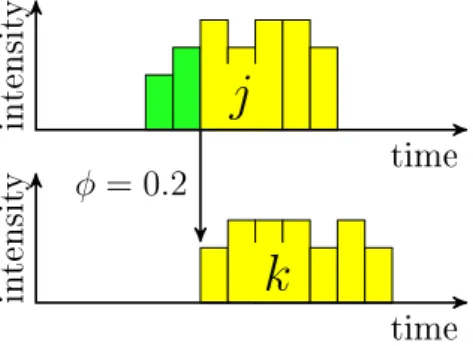
In Section 2.2 the RCPSVP model is extended with feeding precedence constraints. A feeding precedence constraint is described by an ordered triple (j, k, φ), where j, k ∈ J and 0 ≤ φ ≤ 1 is a rational parameter expressing the fraction of j to be completed before k may be started. If φ < 1, then k may start before j nishes, but it is required that the total fraction of j completed up to any time period t cannot be less than that of k, i.e., Pt

τ=rjx_jt ≥ Pt

τ=rkx_kt for all t ∈ [r_j + p^φ_j, d_j] ∩ [r_k, d_k], where p^φ_j is the minimum number of time periods needed to nish the φ fraction of j, i.e., p^φ_j = dφ/hje. Notice that for φ = 1 we get back the familiar end-to-start precedence constraints. For this problem the results of RCPSVP will be generalized and new computational results will be presented.

In Section 2.3 resource leveling problems in a machine environment are discussed. Recall that machines are renewable resources with constant 1 availability, and each activity may require 0 or 1 unit from them. We will consider a multiple-machine environment, where each job is dedicated to a machine, but the starting times of the jobs on each machine have to be determined in order to minimize the objective function (2.1) for linear (2.2) or quadratic (2.3) functions. We will study the complexity of the problem, and determine the borderline between N P-hard and tractable cases.

The content of Section 2.1 is based on Kis [64], that of Section 2.2 on Kis [65], and Section 2.3 presents selected results from Drótos and Kis [29].

2.1 Project scheduling with variable intensity activities

Most results on the resource-constrained project scheduling problem (RCPSP) assume xed activity durations and a constant rate of resource usage while

(9)

2.1. VARIABLE INTENSITY ACTIVITIES 5 performing every activity. Extensions to RCPSP relaxing at least one of these assumptions comprise preemption of activity execution, the discrete time/resource trade-o , the time/cost trade-o and the multi-mode resource- constrained project scheduling problems (see e.g Herroelen et al. [50], Brucker et al. [14] and Demeulemeester and Herroelen [25]). We will study a further extension, called RCPSVP, in which the intensity of each activity may vary over time and the resource-usage is proportional to the intensity.

An instance of the problem is given by a nite set J of activities, a nite set R of continuously divisible renewable resources and a precedence relation E ⊂ J × J among the activities. The time horizon is divided into T unit-length periods, which will be indexed as t = 1, . . . , T. For each activity j ∈ J a release time rj and a deadlinedj specify an interval of time periods {r_j, . . . , d_j} in which the activity must entirely be executed, where 1 ≤ r_j ≤ d_j ≤ T. In each time period t ∈ {r_j, . . . , d_j} at most an h_j ≤ 1 fraction of activity j may be completed. Activity j requires a total of aij

units of resource i, for each i ∈ R. If the intensity of activity j is x_jt in time period t, where 0 ≤ x_jt ≤ h_j and Pdj

t=rjx_jt = 1 hold, then it requires a_ij·x_jt units of resourceiin that period. Each resourcei∈ Rhas an internal capacity of b_it units that is available free of charge, and it has an additional external capacity ofb_it units at the expense ofc_it for each external unit used.

The scheduling problem consists of determining for each activity j an intensity x_jt in each time period t ∈ {r_j, . . . , d_j} such that 0 ≤ x_jt ≤ h_j, Pdj

t=rjx_jt = 1, the precedence constraints among the activities are fullled, the resource demand does not exceed the resource availability (internal + external) in any time period, and the total cost of using external capacity is minimized.

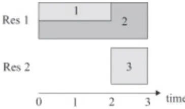
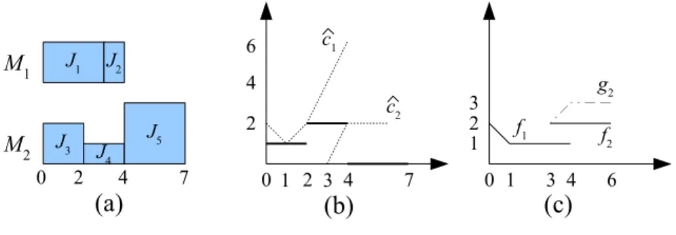
Figure 2.1: Resource usage of activities.

Example 1. To illustrate the above concepts consider a problem instance with 2 renewable resources and 3 activities. All activities have the same time windowrj = 1, . . . , dj = 3, while the maximum intensities areh1 =h2 = 1/2, and h₃ = 1. Activities 1 and 2 require a₁₁ = 1, a₂₁ = 2 unit of resource 1,

(10)

respectively, and activity 3 requires a₃₂ = 1unit of resource 2. The internal capacity of both resources is 1, and there is no external capacity available.

As for precedence constraints, activity 1 must precede activity 3.

The unique solution to this instance is given by the intensity assignments x1 = (1/2,1/2,0), x2 = (1/4,1/4,1/2) and x3 = (0,0,1), respectively, where the t-th component ofx_j represents the intensity of activityj in time period t. Fig. 2.1 depicts the resource usage of the activities with respect to x.

2.1.1 Previous work

Project scheduling with variable intensity activities has been studied by several authors. Weglarz [104] proposes a continuous time model for alloca- ting a single, doubly constrained resource to a set of activities over time, the objective being to minimize project duration. The single resource may be allocated to activities in arbitrary amounts within given intervals. The performance-speed or intensity of each activity is determined by a continuous, non-decreasing function of the amount of resource allocated to it at any moment. Weglarz provides several analytical results and discusses a few numerical examples. Leachman et al. [78] study a discrete time version of the model of Weglarz in which all the dierent types of resources required by an activity are applied proportionally to the (varying) intensity of the activity. The authors propose a heuristic algorithm for minimizing the makespan. For modeling and solving the special case where all lower bounds on activity intensities are 0, Tavares [99], [100] suggests a non-linear program, containing products of decision variables, which is solved by a standard non- linear optimization software. Finally, Hans [47] discusses in Chapter 6 of his Ph.D. thesis exactly the same model which is the topic of this section. His approach is branch-and-price, which is dual to our branch-and-cut approach.

Hans obtains an initial upper bound by various constructive heuristics based on LP rounding techniques and by iterative improvement. In the column generation phase he uses a fast pricing algorithm and also rounding heuristics to obtain feasible solutions.

2.1.2 Summary of main contributions

We propose a new mixed integer-linear program formulation of RCPSVP, where the novelty lies in the modeling of the precedence constraints (Section 2.1.3).

It is also shown how other objective functions t in our framework. The pro's and con's of the alternative formulations are discussed in Section 2.1.4. In Section 2.1.5 we prove that RCPSVP is N P-hard in the strong sense. In

(11)

2.1. VARIABLE INTENSITY ACTIVITIES 7 Section 2.1.6, we analyze the polytope K_jk of all feasible intensity assignments to a pair of variable-intensity activities j and k with (j, k)∈ E. This polytope is decomposed into two smaller dimensional polytopes which, in fact, are instances of the same polytope K. Valid inequalities for K along with a separation algorithm is provided next. In Section 2.1.7 we show that the inequalities found previously completely describe the convex hull of K and also that of Kjk and establish conditions under which the inequalities represent facets of these polytopes. In Section 2.1.8 we describe a branch- and-cut algorithm based on our polyhedral results and summarize various computational experiments with it. In particular, we compare our method to that of Hans for RCPSVP and also a variant of our method to the approach of Tavares for minimizing the makespan.

2.1.3 New formulations

Since resources must be allocated to activities over discrete time periods, it is natural to use a time-indexed formulation with the following variables:

xjt = intensity of activity j in time period t,

z_jt = mask of activityj in time period t. z_jt = 1 if activity j may be executed in time period t and 0 otherwise,

yit = external capacity of resource i∈ R used in time period t. Let p_j = d1/h_je denote the minimum time to complete activity j. Now suppose (j, k)∈ E, i.e., activity j must complete before activity j may start.

Since activityj cannot complete beforer_j+p_j, w.l.o.g. we may assume that r_j+p_j ≤r_k. Similarly, activity j must complete not later than d_k−p_k, that is, we may assume that dj ≤ dk −pk. After these preliminaries, the weak formulation for RCPSVP is as follows:

Minimize X

i∈R

X

t∈{1,...,T}

cit·yit

subject to

dj

X

t=rj

x_jt = 1, j ∈ J, (2.4a)

x_jt ≤h_j·z_jt, j ∈ J, t∈ {r_j+p_j, . . . , d_j} (2.4b) xkt≤hk·(1−zjt), (j, k)∈ E, t∈ {rk, . . . , dj} (2.4c) z_jt ≥z_j,t+1, j ∈ J, t∈ {r_j +p_j, . . . , d_j −1}, (2.4d)

(12)

X

j: rj≤t≤d_j

a_ij ·x_jt ≤b_it+y_it, i∈ R, t∈ {1, . . . , T}, (2.4e) 0≤y_it≤b_it, i∈ R, t∈ {1, . . . , T} (2.4f) 0≤x_jt ≤h_j, j ∈ J, t∈ {r_j, . . . , d_j} (2.4g) z_jt ∈ {0,1}, j ∈ J, t∈ {r_j +p_j, . . . , d_j} (2.4h) The objective is to minimize the weighted sum of external capacity used.

By (2.4a), every activity must entirely be executed between its release time and deadline. The precedences between the activities are forced by (2.4b) (2.4d). That is, activity j can be executed at time t only if z_jt = 1 (cf.

(2.4b)). However, when z_jt = 1, no activity k with (j, k) ∈ A may be executed, due to (2.4c). Finally, (2.4d) ensures that there is a time point t₀ ∈ {r_j +p_j, . . . , d_j + 1} such that z_jt = 1 for all t ∈ {r_j +p_j, . . . , t₀ −1}

and z_jt = 0 for all t ∈ {t₀, . . . , d_j}, hence, activity j has to complete before activity j may start. Since activity j cannot complete before r_j +p_j, we have no z_jt variables for t ∈ {r_j, . . . , r_j +p_j −1}. The external capacity y_it of resource i used in time period t is determined by (2.4e) and it cannot be more than b_it, due to (2.4f). Finally, the domains of the variables x_jt and z_jt are given by (2.4g) and (2.4h), respectively.

If activityjhas no successors inE, thenz_jt can be set to 1 for allt∈ {r_j+ p_j, . . . , d_j}, and similarlyy_itcan be set to 0 if no activity may require resource iat timet, i.e.,t /∈ {r_j, . . . , d_j}for allj ∈ J witha_ij >0. A further reduction is possible for (j, k)∈ E. Since j precedes k, the dierencez_kt−z_jt must be 0 or 1 in any feasible solution. Hence, the inequalities x_kt ≤h_k·(z_kt−z_jt), t ∈ {r_k+p_k, . . . , d_j}, are satised by all feasible solutions and are stronger than (2.4b) for activity j and (2.4c) for (j, k) together. Therefore, we may replace (2.4b) and (2.4c) by the following set of inequalities:

x_kt≤







h_k·(1−z_jt), t∈ {r_k, . . . ,min{rk+p_k−1, d_j}}, h_k·(z_kt−z_jt), t∈ {r_k+p_k, . . . , d_j},

h_k·z_kt, t∈ {max{d_j + 1, r_k+p_k}, . . . , d_k}.

(j, k)∈ E (2.4bc) Notice that some of the intervals may be empty depending on the parti- culardj andrk values. We call the resulting program the strong formulation.

Besides minimizing the cost of using external resources, our model is suitable for other criteria as well. In the following three problems the external resource capacities are neglected. The project duration or makespan can be minimized by nding the smallest T (using dichotomic search between some lower and upper bounds), such that when setting all activity deadlines to T, the linear program (2.4) has a feasible solution. When a due-date d˜j is specied for each activity j, we may minimize the maximum tardiness by

(13)

2.1. VARIABLE INTENSITY ACTIVITIES 9 nding the smallest T_max such that system (2.4) admits a feasible solution with activity deadlinesd_j = ˜d_j+T_max. Again, the minimum value ofT_maxcan be found by dichotomic search. In addition, when weightsw_j are also given, we can minimize the weighted tardiness P

jw_j(max{0, C_j−d˜_j}), whereC_j is the completion time of activity j. That is, dene new weightsw_jt as follows:

w_jt = 0ift≤d˜_j andw_jt =w_j for allt∈ {d˜_j+ 1, . . . , T}. Then, the minimum value of P

wjt·zjt is the minimum weighted tardiness with respect to time horizon T.

The polyhedral results and the branch-and-cut approach presented in this paper can be used to solve the RCPSVP with respect to any of the above optimization criteria.

2.1.4 Comparison of alternative formulations

In this section we discuss the advantages and disadvantages of the alternative formulations for RCPSVP, the emphasis being on integer-linear programming approaches. As all approaches model the resource constraints in essentially the same way, we focus on the modeling of precedence constraints.

Suppose activityj must precede activity k, i.e., (j, k)∈ E. Tavares [100]

models this situation by a set of constraints equivalent to the following:





dj

X

t=t0

x_jt



x_k,t₀ = 0, ∀ t₀ ∈ {r_k, . . . , d_k}.

Tavares shows that the project duration can be minimized by dening new auxiliary variables z_t with 0 ≤ z_t ≤ 1, t ∈ {1, . . . , T}, and adding the constraints

X

j∈J T

X

t=t0

x_jt

!

z_t₀ = 0, ∀ t₀ ∈ {1, . . . , T}.

to the model. Notice that ifzt0 >0, then no activity can be performed after t₀. Therefore, the above constraints along with the objectivemin(T −P

tz_t) express the makespan minimization problem. Since the constraints are clearly non-linear in the variables x and z, Tavares used a non-linear optimization software for solving the problem w.r.t. the makespan objective.

In contrast, Hans [47] models the precedence constraints using a set of binary vectors{β^π ∈ {0,1}^{|J |×T} |π∈Π}consisting of the supports of all feasible intensity assignments to the activities. Although Hans considered distinct projects among which there were no precedence constraints, to simplify notation we assume that all activities belong to the same project. Notice that a binary vectorβ ∈ {0,1}^{|J |×T} is the support of a feasible intensity assignment

(14)

if and only if PT

t=1β_jt ≥ p_j, min{t | β_jt = 1} ≥ r_j, max{t | β_jt = 1} ≤ d_j, and if (j, k)∈ E, thenmax{t|β_jt = 1}<min{t|β_kt= 1}. Clearly, precisely one vector β^π must be chosen. To this end, Hans has introduced new binary variables z_h, h∈Π, together with the following constraints:

X

π∈Π

z_π = 1,

z_π ∈ {0,1}, π∈Π, 0≤x_jt ≤ h_j X

π∈Π

β_i,t^πz_π

!

, ∀j ∈ J, t∈ {r_j, . . . , T}

The rst two constraints ensure that exactly one vector β^π is chosen. The third one species that xjt is either 0, or is between 0 and hj, depending on whether β_it^h is 0 or 1. In addition, Hans' formulation also contains constraints equivalent to (2.4a) and (2.4e), and instead of (2.4f) it has y_it ≥ 0, and P

i∈Ryit ≤bt, for allt, wherebtis a cumulative upper bound for all resources.

As the size of Π can be enormous, column generation is the only viable approach to handle this formulation.

The primary advantage is that any objective function which depends linearly on the cost associated with the vectorβ^π, whatever this cost be, can be optimized by the same solver, provided that the pricing problem can be solved eciently. The main drawback is that a huge number of columns must be handled, and enlarging all activity deadlines by only one time period may multiply the size of Π which may increase considerably the running time of the pricing algorithm.

In contrast, if all activity deadlines are increased by one time period in our formulation, the number of variables grows only by O(|J |+|R|)and the increase in the number of constraints is in O(|J |+|R|+|E|). The drawback is that good cutting planes must be supplied to the solver. Nevertheless, for the objective function studied in this paper our method is competitive with that of Hans, see Section 2.1.8.

2.1.5 Computational complexity

In this section we will prove that RCPSVP is NP-complete in the strong sense.

To this end, we will show that RCPSVP contains the preemptive owshop scheduling problem (PFSP) as a special case. As the latter problem has been shown NP-complete in the strong sense by Gonzalez and Sahni [39], our claim follows. For fundamental denitions and results of scheduling theory see e.g. Graham et al. [40] and Blazewicz et al. [8].

(15)

2.1. VARIABLE INTENSITY ACTIVITIES 11 Recall that in a preemptive owshop a nite set of jobs, J B, must be processed by a nite set of m processors, M. A processor can process at most one job at a time. The processing time of job k on processor iis given by a positive integer number π_ik specifying that jobk must be processed for exactly p_ik time units on processor i. If p_ik = 0 then job k is not processed by processor i. The processing of a job may be interrupted at any (integral) time point and resumed later. Each job k must visit the processors in the same order, that is, if p_i₁_,k >0, p_i₂_,k >0, and i₁ precedes i₂ in the order of processors, then job k must be processed for a total of p_i₁_,k time units on processori1 before its processing may be started on processori2. All jobs can be started at time 1 and the question is whether all jobs can be completed by a given time point C.

A solution σ to the PFSP species the time points in which a job is being processed by a processor. That is, σ(k, i, t) = 1 if job k is processed by processor i in the interval [t, t+ 1] (t is an integer), and 0 otherwise. A solution is feasible if and only if it satises the following conditions:

(i) P

tσ(k, i, t) = p_ik for all jobs k and processors i, (ii) P

kσ(k, i, t)∈ {0,1}for all processors i and time periods t,

(iii) max{t|σ(k, i₁, t) = 1}<min{t⁰ |σ(k, i₂, t⁰) = 1}for all jobskand pairs of processors i₁, i₂ such that i₁ precedes i₂ in the order of processors, and p_i₁_,k, p_i₂_,k >0 hold.

Below we describe a transformation f from PFSP to RCPSVP. Let I be an instance of PFSP, in the corresponding instance f(I) of RCPSVP the set of resources R coincides with the set of processors M. The set of activities J contains an activity for each job-processor pair such that the job has a positive processing time on the processor. The precedence relationE species the processing order of the activities, i.e., E consists of all the pairs (j, j⁰) of activities such that j and j⁰ represents the processing of some job k on consecutive processors. If activity j represents the processing of job k on processor i (when p_ik > 0), then the maximum intensity of activity j is h_j = 1/p_ik, and it requires a_ij = p_ik units of resource (processor) i and no other resources. All activities can be started in time period 1 and they must all be completed at latest in time period C. The internal capacity of each resource is 1 in each time period and its external capacity is always 0. We have the following:

Lemma 1. [64]^∗An instanceI of PFSP admits a feasible solution if and only if the corresponding instance f(I) of RCPSVP admits a feasible solution.

(16)

Proof. Suppose rst that the instance of PFSP has a solutionσ. If activityj represents the processing of job k on processori then set x_jt =σ(k, i, t)/π_ik. Moreover, set z_jt = 1 if and only if there exists t⁰ ≥ t with x_jt⁰ > 0, and 0 otherwise. Finally, set y_it = 0 for all resources (processors) i and time periods t. One can verify that the above (x, y, z)satises system (2.4).

Conversely, suppose system (2.4) admits a feasible solution(x⁰, y⁰, z⁰). We will prove that in this case there exists a possibly dierent feasible solution (x, y, z) of the system such that xjt =hj or 0, y =y⁰ and z =z⁰. From this claim it follows that the schedule σ, dened by σ(k, i, t) = x_jt/h_j for each k, i, tand j such that activityj represents the processing of jobk by processor i, is a feasible solution for the PFSP instance. It is enough to verify property (ii), as the other two requirements of feasible schedules easily follow from the properties of feasible solutions of system (2.4). We have the following estimation on the number of jobs requiring a processor iin time period t:

X

k

σ(k, i, t) = X

j

x_jt/h_j = X

j:aij>0,t∈{r_j,...,dj}

a_ij ·x_jt ≤1.

Here, the second summation is over all activitiesj representing the processing of a job k by processor (resource) i. The second equation follows from the denition of hj and aij and the inequality is due to the fact that (x, y, z) satises (2.4e) and y must be all 0 since all external resource capacities are 0.

To prove our claim, observe that in any feasible solution of (2.4),z is a 0/1 vector. LetU^j be the subset of time points where activityj may be executed, i.e., z_jt = 1 andz_j⁰_,t = 0 for all j⁰ such that (j⁰, j)∈ E (cf. constraints (2.4b) and (2.4c)). Since all components of z are xed to 0 or 1, we may rewrite the system (2.4) as follows:

dj

X

t=rj

x_jt = 1, ∀j ∈ J, (2.5a)

X

j:aij>0

(1/h_j)·x_jt ≤1, ∀i∈ R, t∈ {1, . . . , T} (2.5b) 0≤xjt ≤hj, ∀j ∈ J, t∈U^j (2.5c)

x_jt = 0, j ∈ J, t /∈U^j. (2.5d)

Multiply the constraints (2.5a),(2.5c) and (2.5d) by 1/hj and replace (1/h_j)·x_jt by a new variable x˜_jt. The resulting system, depicted below,

(17)

2.1. VARIABLE INTENSITY ACTIVITIES 13 is a transportation problem.

dj

X

t=rj

˜

x_jt = 1/h_j, j ∈ J (2.6a)

X

j:aij>0

˜

x_jt ≤1, ∀i∈ R, t ∈ {1, . . . , T} (2.6b) 0≤x˜jt ≤1, i∈J, t∈U^j (2.6c)

˜

x_jt = 0, j ∈ J, t /∈U^j. (2.6d)

Since the constraint matrix of (2.6) is totally unimodular and the right hand side is integral (since every h_j is the inverse of some p_ik ∈ Z⁺), the Homan-Kruskal theorem on unimodular matrices [51] implies that there exists an integral solution x. Sincex_jt is between 0 and 1, x is a 0-1 vector.

Then, x_jt =h_j·x_jt is a solution of (2.5) such that x_jt = 0 or h_j, as claimed.

Before proving strong NP-completeness of RCPSVP notice that the maximum numbers Max[I] and Max⁰[f(I)] in an instance I of PFSP and in the corresponding instancef(I)of RCPSVP, respectively, are the same, i.e., both have the value max{maxp_ij, C}.

Corollary 1. [64]^∗RCPSVP is NP-complete in the strong sense.

Proof Membership in NP is straightforward. To show strong NP-completeness it suces to verify thatf is a pseudo-polynomial transformation (Garey and Johnson [36], p. 101) from PFSP to RCPSVP. Namely, an instance I of PFSP admits a feasible solution if and only if the corresponding instance f(I) of RCPSVP has a feasible solution, by Lemma 1. Moreover, f can be computed in time polynomial in the length of I and Max[I]. The length of f(I) is not smaller than the length of I and Max⁰[f(I)] is bounded by a two-variable polynomial in the length of I and Max[I], since they are the same.

As a consequence, RCPSVP cannot be solved in pseudo-polynomial time, unless P=NP. Hence, we will propose a branch-and-cut algorithm using strong valid inequalities which is the topic of the next section.

2.1.6 Polyhedral results for RCPSVP

If we omit the resource capacity constraints (2.4e) from the weak (or from the strong) formulation of RCPSVP, then the feasible solutions of the remaining system are all the intensity assignments to activities respecting the release

(18)

times, deadlines, maximum intensities and precedence constraints. We may consider this system as a collection of subsystems each describing the feasible intensity assignments to a pair of activities connected by a precedence constraint. In this and the next section we will obtain a complete description of the polytope associated with such a subsystem.

Feasible intensity assignments to a pair of activities

Letj, kbe a pair of activities with(j, k)∈ E. Ifdj < rk, then this precedence constraint is meaningless, so we may assume that r_k ≤ d_j. Recall also that r_j +p_j ≤ r_k and d_j ≤ d_k−p_k. We dene the polytope K_jk as the convex hull of all feasible intensity assignments to j and k such that j completes before k starts. That is, K_jk is the convex hull of all points (x_j, x_k, z_j) ∈ R^s^j×R^s^j× {0,1}^s^j^−p^j, wheres_j =d_j−r_j+ 1and s_k =d_k−r_k+ 1, satisfying the following constraints:

dj

X

t=rj

x_jt = 1, (2.7a)

0≤x_jt ≤h_j, t∈ {r_j, . . . , r_j+p_j−1} (2.7b) 0≤x_jt ≤h_j·z_jt, t∈ {r_j +p_j, . . . , d_j} (2.7c) zjt ≥zj,t+1, t∈ {rj+pj, . . . , rk−1} (2.7d) z_jt ≥z_j,t+1, t∈ {r_k, . . . , d_j−1} (2.7e)

d_k

X

t=rk

x_kt= 1, (2.7f)

0≤x_kt≤h_k·(1−z_jt), t∈ {r_k, . . . , d_j} (2.7g) 0≤x_kt≤h_k, t∈ {d_j + 1, . . . , d_k} (2.7h) In order to nd a linear representation ofK_jk consider the polytopesK_j∗

and K∗k derived from K_jk as follows:

Kj∗ = conv

(x_j, z_j)∈R^s^j × {0,1}^s^j^−p^j | (x_j, z_j)satises (2.7a)−(2.7e) , K∗k= conv

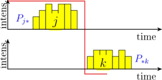
(x_k,z˜_j)∈R^s^k× {0,1}^d^j^−r^k⁺¹ | (x_k,z˜_j) satises(2.7e)−(2.7h) . A feasible intensity assignment to a pair of acitivities is shown in Figure 2.2.

The main result of this section is the following:

Lemma 2. [64]^∗Let (x_j, x_k, z_j) be any point in R^s^j ×R^s^k ×R^s^j^−p^j. Then (xj, xk, zj) ∈ Kjk if and only if (xj, zj) ∈ Kj∗ and (xk,z˜j) ∈ K∗k, where

˜

z_jt =z_jt for all t∈ {r_k, . . . , d_j}.

(19)

2.1. VARIABLE INTENSITY ACTIVITIES 15

Pj∗

j

P∗k

intens. time

k

intens. time

Figure 2.2: Feasible intensity assignment to a pair of activities (j, k)∈ E. Before the proof we derive some common properties ofKj∗ and K∗k. In fact, Kj∗ and K∗k are both equivalent to the polytope K dened next. Let 1 ≤ m < n be integer numbers, and 0 < h ≤ 1 a real number such that (n−m)h≥1. Then K is the convex hull of all points (x, z)∈Rⁿ× {0,1}^m satisfying the following linear constraints:

n

X

t=1

x_t = 1 (2.8a)

xt ≤ h·(1−zt), t∈ {1, . . . , m} (2.8b) x_t ≤ h, t∈ {m+ 1, . . . , n} (2.8c) z_t ≥ z_t+1, t∈ {1, . . . , m−1} (2.8d)

x_t ≥ 0, t∈ {1. . . , n}. (2.8e)

We obtain a polytope equivalent toKj∗ by the substitutionsm=s_j−p_j, n = s_j, h = h_j, z_t = 1− z_j,d_j−t+1, t ∈ {1, . . . , m}, and x_t = x_j,d_j−t+1, t ∈ {1, . . . , n}. We get a polytope equivalent toK∗kby settingm=dj−rk+1, n = s_k, h = h_k, z_t = ˜z_j,t+r_k−1, t ∈ {1, . . . , m}, and x_t = x_k,t+r_k−1, t ∈ {1, . . . , n}.

A necessary and sucient condition for a vector (x, z)∈Rⁿ×R^m to be in K is provided next. First of all, if(ˆx,z)ˆ is a vertex of K, thenzˆis one of the following vectors z^` ∈ {0,1}^m:

z^`_t =

1 if t∈ {1, . . . , `−1},

0 if t∈ {`, . . . , m}, `∈ {1, . . . , m+ 1}.

Moreover, if zˆ=z^` for some vertex (ˆx,z)ˆ and some `, then xˆt= 0 for all t ∈ {1, . . . , `−1}, 0 ≤ xˆ_t ≤ a for all t ∈ {`, . . . , n} and Pn

t=1xˆ_t = 1. After these preparations, we can prove the following:

Lemma 3. [64]^∗Let (x, z) be any point in Rⁿ×R^m. Then (x, z)∈K if and only if the numbersλ₁ = 1−z₁, λ_` =z`−1−z_` (` ∈ {2, . . . , m})andλ_m+1 =z_m

(20)

are all non-negative and there exist vectors x^` ∈Rⁿ, `∈ {1, . . . , m+ 1}, such that Pm+1

`=1 λ_`x^` =x and every (x^`, z^`) belongs to K.

Proof. (Necessity) If (x, z) is a point in K and the points (ˆx^θ,zˆ^θ), θ ∈ Θ, constitute the set of vertices of K, then there exist reals ωθ ≥ 0 such that (x, z) = P

θ∈Θω_θ(ˆx^θ,zˆ^θ), P

θ∈Θω_θ = 1. Let λ_` = P

θ:ˆz^θ=z^`ω_θ, ` ∈ {1, . . . , m+ 1}. Then λ_` ≥ 0 and P

`λ_` = 1. If λ_` > 0, let x^` = P

θ:ˆz^θ=z^`(ω_θ/λ_`)ˆx^θ. Otherwise, if λ_` = 0, choose an arbitrary x^` such that (x^`, z^`) ∈ K. Then every (x^`, z^`) belongs to K and P

`λ_`(x^`, z^`) = (x, z). Using this and the fact that z_m^` = 1 if and only if

` =m+ 1, λ_m+1 =z_m follows. An inductive argument proves that the rest of the λ_` must also equal the specied values.

(Suciency) Observe thatPm+1

`=1 λ_`= 1 and also Pm+1

`=1 λ_`z^` =z. Conse- quently, if there exist vectors x^` satisfying the conditions of the lemma, then (x, z)is a convex combination of the points(x^`, z^`). Since the vectors(x^`, z^`) all belong to K,(x, z)∈K.

Proof of Lemma 2 By the denitions, if (x_j, x_k, z_j)∈K_jk, then (x_j, z_j)∈ Kj∗ and (x_k,z˜_j)∈K^∗k, where z˜_jt =z_jt for all t∈ {r_k, . . . , d_j}.

Conversely, suppose (xj, zj)∈Kj∗ and (xk,z˜j)∈K∗k, where z˜jt =zkt for all t ∈ {r_k, . . . , d_j}. In order to apply the previous lemma to Kj∗ and K∗k, dene the vectors z_j^` ∈ {0,1}^s^j^−p^j and z_k^` ∈ {0,1}^d^j^−r^k⁺¹ as follows.

z_jt^` =

1 if t ∈ {r_j +p_j, . . . , `−1},

0 if t ∈ {`, . . . , d_j} `∈ {r_j +p_j, . . . , d_j + 1}.

For each `∈ {r_k, . . . , d_j + 1}, let z_kt^` =z_jt^` for all t ∈ {r_k, . . . , d_j}.

Applying Lemma 3 toKj∗ yields vectorsx^`_j and coecients λ`,` ∈ {rj+ p_j, . . . , d_j + 1} such that Pdj+1

`=rj+pjλ_`(x^`_j, z_j^`) = (x_j, z_j), (x^`_j, z^`_j) ∈ Kj∗ for each `, λ_r_j_+p_j = 1−z_r_j_+p_j, λ_` = z_j,`−1 −z_j`, ` ∈ {r_j +p_j + 1, . . . , d_j}, and λ_d_j₊₁ =z_j,d_j.

For K∗k we get vectors x^`_k and coecients α_`, ` ∈ {r_k, . . . , d_j + 1} such that Pdj+1

`=rkα_`(x^`_k, z_k^`) = (x_k,z˜_j), (x^`_j, z_j^`) ∈ K_∗k for each `, α_r_k = 1−z˜_j,r_k, α_` = ˜zj,`−1−z˜_j,`, `∈ {r_k+ 1, . . . , d_j}, and α_d_j₊₁ = ˜z_j,d_j.

Since z_jt = ˜z_jt, t ∈ {r_k, . . . , d_j} by assumption, it follows that α_` = λ_`,

` ∈ {r_k+ 1, . . . , d_j + 1}, and α_r_k = 1−Pdj+1

`=rk+1λ_` =Prk

`=rj+pjλ_`.

Lettingx^`_k =x^r_k^k for each `∈ {r_j +p_j, . . . , r_k−1}, we have (x_j, x_k, z_j) = Pdj+1

`=rj+pjλ_`(x^`_j, x^`_k, z_j^`). Since each(x^`_j, x^`_k, z_j^`)belongs toK_jk by the denition of the polytopes Kj∗ and K∗k, (x_j, x_k, z_j)∈K_jk as well.

Corollary 2. [64]^∗If Kj∗ = {(xj, zj) | A^j∗xj +B^j∗zj ≤ b^j∗} and K∗k = {(x_k,z˜_j) | A^∗kx_k+B^∗kz˜_j ≤ b^∗k}, then K_jk = {(x_j, x_k, z_j) | A^j∗x_j +B^j∗z_j ≤

(21)

2.1. VARIABLE INTENSITY ACTIVITIES 17 b^j∗, A^∗kx_k + [0, B^∗k]z_j ≤ b^∗k}, where 0 is a null matrix with r_k −r_j − p_j columns and appropriate number of rows.

We will provide a minimal linear representation of K in Section 2.1.7, which can trivially be transformed to one for K_j∗ and for K_∗k, respectively.

We will prove that putting together these two representations yields a minimal linear representation of K_jk.

Relation to xed-charge network ows

In [89], the xed charge network (or variable upper-bound) ow model is dened. That is, P₌ = conv{(x, z) ∈ Rⁿ× {0,1}ⁿ | Pn

t=1x_t = g,0 ≤ x_t ≤ h_tz_t, t= 1, . . . , n}, wheregand theh_ts are constants. The system dening the polytopeP₌ models a fragment of a network consisting of a node uand arcs entering u. The total ow through the arcs has to meet a specied demand g. The upper bounds on the arcs are variable as they are determined by the binary variables z_t. In the denition of polytope K, there is an ordering on the arcs by the constraints z_t ≥ z_t+1. That is, if z_t₀ is set to 1, then for all t ∈ {1, . . . , t₀} the upper bound on x_t is xed at h and if z_t₀ = 0 then the upper bound is 0 on all arc ows x_t with t ∈ {t₀, . . . , m}. As we will see, these extra constraints yield a new set of facets, dierent to the ow-cover inequalities of [89].

Valid inequalities and a separation algorithm for K

Clearly, the equation (2.8a) and the inequalities (2.8b)-(2.8e) are all valid for K. Moreover, the inequality

z_m ≥0 (2.8f)

is also valid for K. We derive a new class of valid inequalities below.

Denote p = d1/he and hrem = 1−(p−1)h. Since (n −m)h ≥ 1 by denition, m+p≤n.

Lemma 4. [64]^∗Let ∅ 6= S₁ ⊆ {1, . . . , m} and S₂ ⊆ {m+ 1, . . . , n} be such that |S₁|+|S₂| = p and let t₁ be the smallest element of S₁. The (S₁, S₂) inequality

h_remz_t₁ +h X

t∈S1−{t1}

z_t≤ X

t∈{t1,...,n}−(S1∪S2)

x_t (2.8g)

is valid for K.

Proof As K is a convex polytope, it suces to show that any vertex of K satises (2.8g). Since the inequalities are valid for any vertex (ˆx,z)ˆ with

(22)

ˆ

z_t₁ = 0, assumezˆ_t₁ = 1. Therefore,xˆ_t₁ = 0by (2.8b), and the total processing in {t₁, . . . , n} −(S₁ ∪S₂), that is, the right hand side of (2.8g), is at least 1 minus the maximum processing in S₁ ∪S₂ − {t₁}. The latter is h|S₂|+ hP

t∈S₁−{t₁}(1−zˆ_t). Plugging all this together, the statement follows.

The usefulness of the (S1, S2) inequalities is illustrated by the following:

Example 2. Suppose m = 4, n = 7 and h = 2/5. Then p = 3 and h_rem = 1/5. The vector (x, z), where x = (1/10,0,0,3/10,2/5,1/5,0) ∈ R⁷ and z = (3/4,1/2,1/2,1/4) ∈ R⁴, satises (2.8a)-(2.8f), but violates (2.8g) for S₁ ={1,4} and S₂ ={5}. Namely, we have

h_remz₁+hz₄ = 1 5· 3

4 +2 5 ·1

4 = 1 4 > 1

5 = 0 + 0 + 1 5 + 0

=x₂+x₃+x₆+x₇ = X

t∈{1,...,7}−(S1∪S2)

x_t.

We close this section by a separation algorithm for the (S₁, S₂)inequalities. For each t1 ∈ {1, . . . , m}, the procedure tries to nd a violated (S1, S2) inequality with t₁ being the smallest element of S₁. Namely, rewrite (2.8g) as follows:

X

t∈S1−{t1}

(h·z_t+x_t) +X

t∈S2

x_t≤





X

t∈{t1+1,...,n}

x_t



−h_remz_t₁. Now consider the following optimization problem:

max X

t∈S₁−{t₁}

(h·z_t+x_t) +X

t∈S2

x_t, (2.9)

where themaxis over all set pairs(S₁, S₂)such thatt₁ ∈S₁ ⊆ {t₁, . . . , m}, S₂ ⊂ {m+ 1, . . . , n} and |S₁|+|S₂|=p. The maximum is greater than the constantP

t∈{t1+1,...,n}x_t−h_remz_t₁ if and only if at least one(S₁, S₂)inequality with t₁ being the smallest element of S₁ is violated by (x, z).

In order to solve problem (2.9), dene a set of itemsI(t₁) = {t₁+1, . . . , n}

with item weights w(t) = h·zt+xt if t1 + 1 ≤ t ≤ m, and xt if m+ 1 ≤ t ≤ n. Then the p−1 largest-weight items constitute an optimal solution to (2.9). In fact, this problem can be seen as nding a maximum weight basis in the uniform matroid over I(t1) in which everyp−1items is a basis.

Repeating this procedure for each t₁ ∈ {1, . . . , m} we can nd a violated (S₁, S₂) inequality or conclude that none exists.

For ecient implementation notice that the item weights do not depend on t₁ and thus it is enough to sort the elements of the set I(1) in decreasing

(23)

2.1. VARIABLE INTENSITY ACTIVITIES 19 order of their weights. Then, after increasing t₁ by 1, eliminate from the ordered list t₁. By using appropriate data structures, the time complexity of the entire separation procedure is O(nlogn).

Proposition 1. [64] Inequalities (2.8g) can be separated in O(nlogn) time.

2.1.7 Minimal linear representations for K and K

jk

In this section we will prove that the inequalities (2.8a)-(2.8g) constitute a linear representation of K. Moreover, we will establish conditions under which these inequalities represent facets of K. Finally, we will extend these results to K_jk.

A linear representation of K

LetP be the polytope consisting of all points(x, z)∈Rⁿ×R^m satisfying the system (2.8a)-(2.8g). Since the equation (2.8a) and the inequalities (2.8b)- (2.8g) are all valid for K, K ⊆P. Our main goal is to prove the following:

Theorem 1. [64]^∗P ⊆K.

Proof Assuming the contrary, x some (x, z) ∈ P \K. Since (x, z) ∈/ K, it is not a convex combination of points in K. We will show that then (2.8g) is violated for a pair of sets (S1, S2) which contradicts the assumption (x, z)∈P.

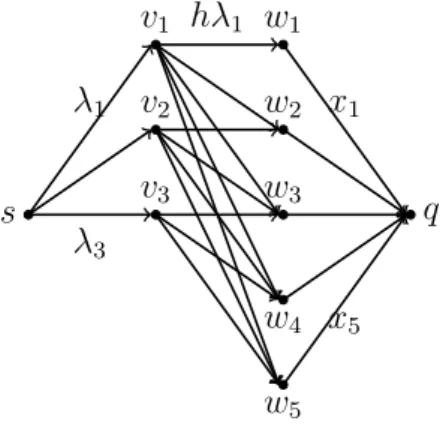
To this end, dene the capacitated network G(x, z) = (V, E) with node setV consisting of a sources, a sink q, a nodev` for each `∈ {1, . . . , m+ 1}

and a node w_t for each t ∈ {1, . . . , n}. The source s is connected to every v_` by one arc (s, v_`) with capacity c(s, v_`) = λ_`, where the λ_` are dened in Lemma 3. Moreover, there is one arc from each wt to sink q with capacity c(w_t, q) =x_t. Finally, for each `∈ {1, . . . , m+ 1} and t ∈ {`, . . . , n}there is an arc(v_`, w_t)with capacity c(v_`, w_t) = h·λ_`. This construction is illustrated in Fig. 2.3. Since (x, z)∈P, all arc capacities in G(x, z) are non-negative.

Letc(δ(S)) =P

(u,v)∈δ(S)c(u, v)denote the capacity of ans−qcutδ(S) = {(u, v) ∈ E | u ∈ S, v ∈ S}, where s ∈ S ⊆ V \ {q} and S = V \S. The minimum capacity of an s−q cut in G(x, z) is at most 1, as c(δ({s})) = P

`λ_` = 1.

Claim 1. The minimum capacity of ans−q cut inG(x, z)is strictly smaller than 1.

Proof Assuming the contrary, it follows that there exists a compatible ow f inG(x, z)of value 1, due to the MAX-FLOW MIN-CUT Theorem of Ford and Fulkerson [31]. For each ` ∈ {1, . . . , m+ 1} dene a vector x^` ∈ Rⁿ as