Case Studies for Improving FMS Scheduling by Lot Streaming in Flow-Shop Systems

Case Studies for Improving FMS Scheduling by Lot Streaming in Flow-Shop Systems

Ezedeen Kodeekha

Budapest University of Technology and Economics Műegyetem rkp. 3, H-1111 Budapest, Hungary Fax: +36-1-463-3271; Tel.: +36-1-463-2945 ezo12@yahoo.com

Abstract: This paper deals with scheduling problems of the Flexible manufacturing systems (FMS). The objective is to improve the utilization of FMS. Lot Streaming (LS) is used to meet this objective.

In this paper a comparative study is performed between the applications of new methods:

Brute Force method (BFM) and Joinable Schedule Approach (JSA). Case studies for Flow Shop Systems (FSS) are performed. Attached independent sequence setup times are considered. It is concluded that these methods can be used effectively to solve LS problems.

In the paper a general optimization mathematical model of LS for FMS scheduling problems of FSS is developed and presented.

Keywords: FMS Scheduling, Scheduling Priority Rules, Lot Streaming, Global Minimum of Production Time, Excess Time Coefficient, Brute Force Method, Joinable Schedule Approach

Abbreviation: CIM: Computer Integrated Manufacturing. CIF: Computer Integrated Factory. FMS: Flexible Manufacturing System. FSS: Flow Shop System. SPR: Scheduling Priority Rules. LS: Lot Streaming. BFM: Brute Force Method. JSA: Joinable Schedule Approach

1 Introduction

Nowadays, in modern manufacturing, Computer Integrated Manufacturing (CIM) is directing the technology of manufacturing towards Computer Integrated Factory (CIF) which is a fully automated factory.

Because CIF would involve a high capital investment, especially in its Flexible Manufacturing System (FMS), efficient machine utilization is extremely essential;

machines must not stand idle. Consequently, proper FMS scheduling is required.

Furthermore, for the industrialized nation, FMS must be able to meet critical challenge: to react quickly to current competitive market conditions. There are

two challenges: maximize utilization and minimize production time. Of course, these quantities are interconnected and highly depend on the quality of scheduling.

So, appropriate FMS scheduling must be analyzed accurately.

FMS Scheduling is a manufacturing function to schedule different machines to different jobs which may have different quantities, different processes, different setups, different process sequences, etc. organized according to a certain priority rule subject to certain constraints in order to meet one or multi-criteria.

This paper deals with FMS scheduling problem of Flow Shop System (FSS) in where all the jobs to be produced follow the same process sequence (path or route).

In this paper, FSS with attached independent sequence setup time is considered.

The objective of this paper, like the earlier ones [10, 11, 12, 13, 14], is to minimize maximum production time (makespan) close to the global minimum of production time in order to improve machine utilization.

The classic methods such as Scheduling Priority Rules (SPR) usually produce schedules with low system utilization.

In this paper, to achieve this objective Lot Streaming (LS) technique is used in which the jobs (batches) are broken and the processes are overlapped concurrently.

Many researchers studied the LS problems. For FSS, there is a lot of literature:

two machines/one job (2/1) Lot Streaming with setup time was given in [1], 2- machines/ multi-jobs (2/J) with setup time was presented in [22, 2, 8], (3/1) was presented in [4], (3/J) in [21], multi-machine group, multi-job (M/J) without setup time in [7, 9], M/J with setup time using Dynamic Programming algorithm in [16], M/J with setup time using Mixed Integer Linear Programming (MILP) in [23], M/J with setup time using Genetic Algorithm (GA) was proposed in [19]. The analysis of batch splitting in an assembly scheduling environment was presented in [18]. Tabu Search (TS) and Simulated Annealing (SA) were proposed in [20].

Comprehensive review of Lot Streaming is presented in [6].

In [10, 11, 12, 13, 14], new methods to solve the LS problems for FMS scheduling were developed. These methods were named as Brute Force Method [BFM] and Joinable Schedule Approach [JSA]. These two methods have different basic ideas and different procedure. BFM is a search method and JSA is an analytical method.

In this paper a comparative study is performed between these methods through case studies for FSS.

1.1 The Content of the Present Paper

This paper begins with an introduction in Section 1 and continues in Section 2 with a problem definition. Case studies are formulated and their engineering database is given in Section 3. In Section 4 applications of Brute Force Method and Joinable Schedule Approach are given and the comparison of the results of the methods is presented. Conclusions can be read in Section 5.

2 Problem Definition

2.1 Problem Statement

The problem considered in this paper is FMS scheduling problem. The FMS consists of different machine groups m (m =1, 2 …M) to process different jobs (bathes) j (j=1, 2…J) in different volumes (number of parts) n1, n2...nj with different processing time of one part of job j on machine group m, this time is indicated by τj,m.

Rather detailed information about the above model can be found in [13].

2.2 Global Minimum of Production Time and the Excess Time Coefficient

Let τj,m be the processing time of one part of job j on machine group m as introduced above. Then, the total load time of machine group m is indicated as Lm

Lm = _j

J j

m

j n

∑

=1

τ

, (1) The load time of the bottleneck machine group, Lb is the maximum load among all loads of the machine groups.

Lb =Max Lm = Max _j

J j

b

j n

∑

=1

τ

, (2) Let

δ

_j,m be the attached independent sequence setup time of machine group m to process job j. Then, the overall setup time for a machine group, when the manufacturing sequences are known, is the sum of set up times of machine group m to process all jobs.

Sm =

∑

= J

j jm

1

δ

, (3) We suppose that the bottleneck machine group has the maximum summation of setup times. So, the total setup times of bottleneck machine group is

Sb = Max Sm =

∑

= J j

b

Max j 1

δ

, (4) The fulfillment of this condition is by far not trivial. But we suppose that it is valid in a number of practical cases and here we deal with these cases.

It is remarkable that the Lm (m = 1, 2 ...M) values for a given order of production do not depend on the order of production sequences. But the Sm (m = 1, 2 ...M) values depend on that. In the present paper we consider known feasible schedules for which the sequences are known, too. So, the setup times sum can be estimated, furthermore, in the case studies, for simplicity, everywhere the same setup time value was used for all parts and for the machine groups but this did not restrict the validity of the results. The number of setups is known and is the same for all of the machine groups (FSS case). In the FMS type production the setup times have small values. So, it seems to us that different relaxing assumptions concerning setup times do not affect too much the quality of system performance.

Returning to the above, the global minimum of production time is

tg = Min tpr = Lb + Sb (5) In this paper, like in the earlier ones [10, 11, 12, 13, 14], a new quantity called Excess time coefficient Cr is introduced to measure the goodness of FMS scheduling system.

Let tpr be the makespan of the system which is the time length of completion time of the last job to leave the system. It can be defined as the maximum of the production time. The makespan is usually indicated in the literature as Cmax (see:

[17, 3]). Here we use for that tpr. Of course, tpr = Cmax.

The excess time coefficient is defined as the ratio of makespan to the global minimum of production time:

Cr =

g pr

t t

(6) High values of Cr mean low utilization of the system. Cr never has a lower value than 1. To decrease Cr, we will use a lot streaming technique.

We remark that for job shop scheduling problems cases may exist where a value close to 1 (with the closeness determined by the setup times) may be realized.

However, the given schedule may not be very easy to find.

For flow shop problems the global minimum of production time is different from the above. It may be determined as outlined in paper [10]. Nevertheless, Cr is a good quantity for comparisons.

2.3 Lot Streaming Technique

According to the lot streaming technique proposed in [10, 11, 12, 13, 14], the production batches are divided into a number of equal sub-batches, N. Then, the sub-batches can be processed in overlapping manner in order to achieve one or more objectives. At that makespan will decrease due to overlapping process but, at the same time, the sum of set up times will increase. For that reason, the problem of lot streaming to be solved is: What is the optimal number of sub-batches? It is a trade-off optimization problem. In this paper, two methods applied in [10, 11, 12, 13, 14] are used:

a) Brute Force Method, BFM b) Joinable Schedule Approach, JSA

For the investigations of the features of these approaches we will use simulation methods.

2.4 Simulation Method

The objectives of using simulation technique based on Scheduling Priority Rules (SPR) for solving the given problem can be outlined as follows:

a) To select the best feasible initial schedule giving a suitable makespan value.

b) To represent Gantt charts.

c) To specify the global minimum of production time.

d) To determine the excess time coefficient.

e) To determine the utilization of the system.

2.5 Brute Force Method, BFM

BFM is a break and test method in which the initial feasible schedule of production batches is broken many times into sub-batches at certain setup time and tested until finding the suitable number of sub-batches. BFM is a search, enumeration, and optimization method.

In this paper we used a simulation computer program as described in [5]. At certain setup time we divided all batches into many possible sub-batches and then testing was made to compare the new number of sub-batches with the previous number until finding the optimum number of sub-batches in which the excess time coefficient is minimum and system utilization is maximum.

2.6 Joinable Schedule Approach, JSA

Figure 1

Gantt chart of 3/ 3 flow shop scheduling problem with idle times

Let us demonstrate the given approach for FSS cases. For demonstration we introduce an example to clarify the idle times of the system and the method how to schedule a flexible manufacturing system (FSS case). FMS consists of three machine groups (M1, M2, M3) to process three jobs (A, B, C) by different processing times. It is a 3/3 scheduling problem. We suppose that the FIFO schedule is the best feasible schedule. The Gantt chart is illustrated in Figure 1.

In Figure 1, Δτf,m, Δτa,m are the front and after idle time of machine group m, respectively.

Δτi,m is the sum of all of the inside (in-between) idle times. The total idle times of the machine groups Δτm is

Δτm = Δτf,m+ Δτi,m+ Δτa,m (7) In FSS, there is no idle time in front of the first machine group and behind (after) the last machine group, Δτf,1 = Δτa,M = 0

The idle time of the bottleneck machine group is

Δτb = Δτf,b+ Δτi,b+ Δτa,b (8)

Δτa,1

Δτa,2

Δτf,3

Δτi,3,2

Δτi,3,1

Δτf,2

a)

b)

Figure 2

Gantt chart of 2/2 flow shop schedule a) Without lot streaming b) With Lot Streaming, N=2

To simplify the model, let us introduce an example illustrated in Figure 2a and b.

In Figure 2 Gantt chart of initial feasible schedule without lot streaming for 2/2 flow shop scheduling problem is given. We assume that the bottleneck machine group is index 1. The idle time of the bottleneck is Δτb, where Δτb = Δτa,b, of course, Δτf,b = Δτi,b = 0. As was given, the global minimum of production time is tg = Lb + Sb

The makespan tpr is

tpr= tg + Δτb (9) From equation (5)

tpr= Lb+ Sb+ Δτb (10) Now, as proposed in [10, 11, 12, 13, 14], we divide the schedule lengths by integer number N. Then, we move the sub-batches together until they touch each other. Clearly, at the given formulation of the problem this is always possible. We remark that for job shop problems this is quite different, and the “Joinable Schedule Approach” can only be used for special schedules which are not very easy to find (see: [12]).

tg

tpr

2 1 A

2 1 A

2 1 B

2 1 B

2

τ

b

Δ

τ

b

Δ

2

τ

b

Δ

tpr(2)

Let us divide the batches into 2 equal-size sub-batches (see Figures 1a and b).

The bottleneck load time value is constant,

2 1 2

1 2

1 2

1 A B B

A + + + = A1+B1= Lb

The setup times of bottleneck machine group becomes 2*nb*δ = 2 Sb

The idle time of bottleneck machine group becomes 2 τb

Δ

So, the makespan function becomes tpr (2)= Lb+ 2 Sb+

2 τb

Δ (11) If the batches are divided into N equal-size sub-batches, the makespan function will change as follows:

tpr (N) = Lb+ N Sb+ N

τb

Δ (12) Equation (12) needs some comment, in fact, when dividing the batches the setup times appear not only in the bottleneck section but in others too, which are forming the

Δτ

_b part. But this has a very little effect on the system performance, and so it can be neglected, as reflected in equations (11) and (12).

Dividing equation (12) by

t

_g , we obtain the following coefficients:

Cr =

g pr

t

t , Ψr =

g b

t

L , θr =

g b

t

S , Φr =

g b

t τ

Δ

(13) Where Cr, Ψr, θr and Φr are called excess time coefficient, bottleneck global coefficient, setup relation coefficient and bottleneck idle time coefficient, respectively.

Equation (12) becomes Cr = Ψr + θr N + Φr

N

1

(14)

To minimize Cr we can differentiate Cr with respect to N and equalize to zero.

1 0

2 =

Φ

−

∂ =

∂

N N

C

r r

r θ (15) The optimum number of sub-batches is

b b r

r

N Sτ

θ

= Δ

= Φ

* (16)

The optimum excess time coefficient is

r r r

Cr^* = Ψ + 2 Φ θ (17) The minimum makespan is

b b b

pr L S

t^* = + 2 Δ τ (18) The optimum excess time coefficient can be determined as

g pr

r t

C t

*

* = (19)

2.7 Utilization and Makespan

One of the most important means to improve productivity of any system is the efficient utilization of the available resources. As mentioned above, the objective of this paper is to improve the system utilization through FMS scheduling system.

A low value of makespan implies high utilization of the machines. Utilization and makespan are interconnected quantities.

Let U be the initial utilization of the system; it can be computed by the following formula:

t pr

M U L

= * (20) Where L is the total load time of the system. It is determined by summation of all the processing times required to process all jobs.

U^* is the optimum utilization of the system achieved using BFM or JSA to solve lot streaming problem, and can be computed as follow:

*

*

* t_pr M

U = L (21)

To evaluate the improvement of the schedule quality, we use the productivity improvement rate η

η = U

U

U ^* − *100 (22)

3 Case Studies Characterization

In this paper, we analyze 7 different cases of LS problems of FMS scheduling for FSS, each case is characterized as a category S/M/J/mb/O/δ, where S is the type of the system, M is the number of machine groups, J is the number of jobs, mb is the bottleneck machine group index, O is the objective or criterion to measure the performance of the system, δ is the setup time.

The case studies data are introduced in Table 1: To demonstrate the content of the table we give an example which is the first case: FSS/2/2/1/U/2: The flexible manufacturing system is a Flow Shop System consists of two machine groups (M=2) to be processed two jobs (J=2), and the bottleneck machine group index is 1 (mb =1), The objective is to obtain higher utilization U, the setup time (δ=2h).

By using LS technique and applying the two new methods, BFM and JSA, for two Scheduling Priority Rules (SPR), First In

First Out (FIFO) and Minimum Slack (MS), we can find out the optimal quantities of:

number of sub-batches, makespan, Excess time coefficient, utilization and Productivity improvement rate.

We can recognize from Table 1 that cases 1, 2 have same M/J, δ and L but different mb

and Lb. Cases 3, 4 have same M/J, δ, L and Lb

but different mb.

Table 1

Seven case studies of FSS with different machine group index

3.1 Engineering Database of Case Studies

Case No 1: FSS/2/2/1/U/2

Machine group m

1 2

Job j n_j

τ t k τ t k

T_i 1(A) 150 0.67 100 1 0.40 60 2 160 2(B) 200 0.40 80 1 0.20 40 2 120

Lj 180 100 280

Table 2 Database case No 1

Case M/J mb Lb δ L 1 2/2 1 180 2 280 2 2/2 2 160 2 280 3 3/3 1 200 2 500 4 3/3 2 200 2 500 5 3/4 2 320 3 840 6 4/4 3 380 3 1180 7 5/4 5 360 4 1360

Case No 2: FSS/2/2/2/U/2

Machine group m

1 2

Job j nj

τ t k τ t k

Ti

1(A) 200 0.40 80 1 0.50 100 2 180 2(B) 150 0.27 40 1 0.40 60 2 100

L_j 120 160 280

Table 3 Database of case No 2

Case No 3: FSS/3/3/1/U/2

Machine group m

1 2 3

Job j nj

τ t k τ t k τ t k

Ti

1(A) 100 0.40 40 1 0.40 40 2 0.20 20 3 100 2(B) 150 0.40 60 1 0.40 60 2 0.27 40 3 160 3(C) 150 0.67 100 1 0.53 80 2 0.40 60 3 240

Lj 200 180 120 500

Table 4 Database of case No 3

Case No 4: FSS/3/3/2/U/2

Machine group m

1 2 3

Job j nj

τ t k τ t k τ t k

Ti

1(A) 100 0.40 40 1 0.40 40 2 0.20 20 3 100 2(B) 150 0.40 60 1 0.40 60 2 0.27 40 3 160 3(C) 150 0.53 80 1 0.67 100 2 0.40 60 3 240

L_j 180 200 120 500

Table 5 Database of case 4

Case No 5: FSS/3/4/2/U/3

Machine group m

1 2 3

Job j nj

τ t k τ t k τ t k

Ti

1(A) 100 0.40 40 1 0.80 80 2 0.60 60 3 180 2(B) 150 0.27 40 1 0.40 60 2 0.40 60 3 160 3(C) 150 0.40 60 1 0.53 80 2 0.53 80 3 220 4(D) 200 0.40 80 1 0.5 100 2 0.5 100 3 280

Lj 220 320 300 840

Table 6 Database of case 5

Case No 6: FSS/4/4/3/U/3

Machine group m

1 2 3 4

Job j nj

τ t k τ t k τ t k τ t k

Ti

1(A) 200 0.50 100 1 0.40 80 2 0.50 100 3 0.40 80 4 360 2(B) 250 0.24 60 1 0.32 80 2 0.40 100 3 0.24 60 4 300 3(C) 300 0.27 80 1 0.20 60 2 0.27 80 3 0.13 40 4 260 4(D) 250 0.24 60 1 0.24 60 2 0.40 100 3 0.16 40 4 260

Lj 300 280 380 220 1180

Table 7 Database of case No 6

Case No 7: FSS/5/4/5/U/4

Machine group m

1 2 3 4 5

Job j nj

τ t k τ t k τ t k τ t k τ t k

Ti

1(A) 100 0.60 60 1 1 100 2 0.80 80 3 0.80 80 4 1 100 5 420 2(B) 150 0.40 60 1 0.53 80 2 0.40 60 3 0.40 60 4 0.53 80 5 340 3(C) 150 0.27 40 1 0.40 60 2 0.53 80 3 0.40 60 4 0.67 100 5 340 4(D) 200 0.20 40 1 0.30 60 2 0.20 40 3 0.20 40 4 0.40 80 5 260 Lj 200 300 260 240 360 1360

Table 8 Database of case No 7

4 Case Studies for BFM and JSA Applications

4.1 Application of BFM

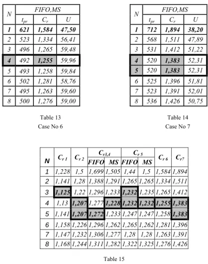
Using LEKIN computer program [17] and applying BFM for the given case studies using another computer program of lot streaming given in [5, 15] we represent the Gantt charts such as in Figures 3 a, b, c of case 7. The values of Cr

and U are presented in Tables 9-14.

a)

b)

c)

Figure 3 Gantt charts of case No 7

a)Without lot streaming b) With lot streaming, N =2 c) With lot streaming, N =4 Improvement

Improvement

4.2 Results of BFM Applications

Table 9 Case No 1

Table 10 Case No 2

Table 11 Cases No 3, 4

FIFO MS N tpr Cr U tpr Cr U 1 478 1,440 58,58 498 1,500 56,22 2 420 1,265 66,67 420 1,265 66,67 3 409 1,232 68,46 410 1,235 68,29 4 409 1,232 68,46 409 1,232 68,46 5 414 1,247 67,63 414 1,247 67,63 6 420 1,265 66,67 419 1,262 66,83 7 425 1,280 65,88 425 1,280 65,88 8 439 1,322 63,78 440 1,325 63,64

Table 12 FIFO,MS

N tpr Cr U 1 226 1,228 61,95 2 210 1,141 66,67 3 207 1,125 67,63 4 208 1,130 67,31 5 210 1,141 66,67 6 213 1,158 65,73 7 211 1,147 66,35 8 215 1,168 65,12

FIFO,MS

N tpr Cr U 1 246 1,500 56,91 2 210 1,280 66,67 3 200 1,220 70,00 4 198 1,207 70,71 5 198 1,207 70,71 6 201 1,226 69,65 7 202 1,232 69,31 8 204 1,244 68,63

FIFO MS N t_pr C_r U t_pr C_r U 1 350 1,699 47,62 310 1,505 53,76 2 286 1,388 58,28 266 1,291 62,66 3 267 1,296 62,42 254 1,233 65,62 4 263 1,277 63,37 253 1,228 65,88 5 262 1,272 63,61 254 1,233 65,62 6 267 1,296 62,42 260 1,262 64,10 7 269 1,306 61,96 263 1,277 63,37 8 270 1,311 61,73 264 1,282 63,13

Table 13 Case No 6

Table 14 Case No 7

C_r3,4 C_{r 5}

N Cr 1 Cr 2

FIFO MS FIFO MS Cr 6 Cr7

1 1,228 1,5 1,699 1,505 1,44 1,5 1,584 1,894 2 1,141 1,28 1,388 1,291 1,265 1,265 1,334 1,511 3 1,125 1,22 1,296 1,2331,2321,235 1,265 1,412 4 1,13 1,2071,2771,228 1,232 1,232 1,255 1,383 5 1,1411,207 1,2721,233 1,247 1,247 1,2581,383 6 1,158 1,226 1,296 1,262 1,265 1,262 1,281 1,396 7 1,147 1,232 1,306 1,277 1,28 1,28 1,263 1,391 8 1,168 1,244 1,311 1,282 1,322 1,325 1,276 1,426

Table 15

Values of excess time coefficient of application BFM for all cases FIFO,MS

N tpr Cr U 1 621 1,584 47,50 2 523 1,334 56,41 3 496 1,265 59,48 4 492 1,255 59,96 5 493 1,258 59,84 6 502 1,281 58,76 7 495 1,263 59,60 8 500 1,276 59,00

FIFO,MS N tpr Cr U

1 712 1,894 38,20 2 568 1,511 47,89 3 531 1,412 51,22 4 520 1,383 52,31 5 520 1,383 52,31 6 525 1,396 51,81 7 523 1,391 52,01 8 536 1,426 50,75

1 1,1 1,2 1,3 1,4 1,5 1,6 1,7 1,8 1,9 2

0 1 2 3 4 5 6 7 8 9 10 N

Cr

Figure 4

Excess time coefficient curves of all cases: Cr, case number, rule

4.3 Application of JSA and its Results

By the substitution of the given values into the equations (5, 9, 16, 18, 21, 22) we can get the results as given in Table 16. From the results given in Table 16 it can be concluded that the productivity improvement rate, for some cases, is high reached to 40.52% and low reached to 9.75%.

CASE RULE Lb Sb tg tpr Δτb N^* t^*pr C^*r U^*% η%

1 FIFO,MS 180 4 184 226 42 3.2 205.9 1.119 67.99 9,75 2 FIFO,MS 160 4 164 246 82 4.5 196.22 1.196 71.34 25,36

FIFO 200 6 206 350 144 4.9 258.78 1.246 64.40 35,24 3 MS 200 6 206 310 104 4.1 249.95 1.213 66.68 24,03 FIFO 200 6 206 350 144 4.9 258.78 1.246 64.40 35,24 4 MS 200 6 206 310 104 4.1 249.95 1.213 66.68 24,03 FIFO 320 12 332 478 146 3.5 403.71 1.215 69.35 18,39 5 MS 320 12 332 498 166 3.7 409.26 1.232 68.41 21,68 6 FIFO,MS 380 12 392 621 229 4.3 484.84 1.236 60.84 28,08 7 FIFO,MS 360 16 376 712 336 4.5 506.64 1.355 53.68 40,52

Table 16 Cr, 7

Cr, 6

Cr, 5MS

Cr, 5FIFO

Cr, 3, 4MS

Cr, 3, 4FIFO

Cr, 2

Cr,1

Case Rule N^*(JSA) N^*(BFM) C^*_r(JSA) C^*_r(BFM) 1 FIFO,MS 3.2 ≈ 3 3 1,119 1,125 2 FIFO,MS 4.5 ≈ 5 4-5 1,196 1,207 FIFO 4.9 ≈ 5 5 1,246 1,272 3 MS 4.1 ≈ 4 4 1,213 1,228 FIFO 4.9 ≈ 5 5 1,246 1,272 4 MS 4.1≈ 4 4 1,213 1,228

FIFO 3.5 ≈ 4 3-4 1.215 1,232 5 MS 3.7 ≈ 4 4 1,232 1,232 6 FIFO,MS 4.3 ≈ 4 4 1,236 1,255 7 FIFO,MS 4.5 ≈ 5 4-5 1,355 1,383

Table 17

Optimal excess time coefficient values of BFM and JSA for all cases

4.4 Comparing the BFM and JSA Results

In Table 17, the values of Cr for seven cases for both rules FIFO and MS applying both methods BFM and JSA are presented.

The values of optimum number of sub-batches N^* for JSA are rounded to closed integer value.

1 1,1 1,2 1,3 1,41,5 1,6 1,7 1,8 1,92

1 2

3FIFO 3M S

4FIFO 4M

S 5FI

FO 5M

S 6 7

Case Cr

Figure 5

Optimal excess time coefficient curves BFM and JSA

Conclusions

From Table 17 and Figure 5 we can conclude that BFM and JSA can be used effectively to solve lot streaming problems of FSS. The application of both methods BFM and JSA gives almost the same results.

JSA can be used for FSS without modifying the initial feasible schedule, and there is no need for joinability test.

BFM curve JSA curve

The optimization mathematical model of JSA developed can be used as a general optimization model of Lot Streaming used for FMS scheduling problem of Flow Shop System with an attached independent sequence setup time.

The data applied in the case studies examples are quite general. So, it may be supposed that the results are widely applicable. Namely, the analytical results obtained by JSA can be easily obtained for extended applications.

References

[1] Baker K. R: Lot Streaming in Two-Machine Flow Shop with Set up Time, Annual of Operations Research 57, 1995, pp. 1-11

[2] Cetinkaya, F. C.: Lot Streaming in a Two-Stage Flow-Shop with Set up Processing and Removal Times Separated, Journal of the Operational Research Society 45(12), 1994, pp. 1445-1455

[3] French S., B. A., M. A. and D. Phil.: Sequencing and Scheduling: An Introduction to the Mathematics of the Job-shop, Ellis Horwood Ltd.

England, 1982

[4] Glass C. A., Gupta J. N. D. and Potts C. N.: “Lot Streaming in Three-Stage Production Processes” European Journal of Operations Research, 75, 1994, pp. 378-394

[5] J. Somló, A. V. Savkin, A. Anufriev, T. Koncz: Pragmatic Aspects of the Solution of FMS Scheduling Problems Using Hybrid Dynamical Approach, Robotics and Computer-Integrated Manufacturing 20, 2004, pp. 35- 47 [6] J. H. Chang, H. N. Chiu: A Comprehensive Review of Lot Streaming”

International Journal of Production Research 43, 2005, pp. 1515-1536 [7] Kalir A., Sarin C.: Evaluation of the Potential Benefits of Lot Streaming in

Flow Shop Systems, International Journal of Production Economics 66, 2000, pp. 131-142

[8] Kalir A., Sarin C.: Constructing Near Optimal Schedules for the Flow Shop Lot Streaming Problem with Sublot-Attached Setups, Journal of Combinatorial Optimization 7(1), 2003, pp. 23-44

[9] Kalir A. A., Sarin S. C.: A Near-Optimal Heuristic for the Sequencing Problem in Multiple-Batch Flow-Shops with Small Equal Sublots, Omega 29, 2001, pp. 577-584

[10] Kodeekha Ezedeen, János Somló: Improvement of FMS Scheduling Efficiency by Optimal Lot Streaming for Flow Shop Problems, in proceedings of 6^th National Conference, BUTE, Budapest, Hungary, May 29-30, 2008

[11] Kodeekha Ezedeen and János Somló: Improving FMS Scheduling by Lot Streaming, Journal of Periodica Polytechnica Series, BUTE, 51.1, 2007, pp. 3-14

[12] Kodeekha Ezedeen, János Somló: Optimal Lot Streaming for a Class of FMS Scheduling Problems-Joinable Schedule Approach, in Proceedings of 11^th IFAC International Symposium on Computational Economics &

Financial and Industrial Systems, Istanbul, Turkey, 2007, pp. 363-368 [13] Kodeekha Ezedeen, János Somló J.: Optimal Lot Streaming for FMS

Scheduling of Flow Shop Systems, in proceedings of 12^th International Conference on Intelligent Engineering Systems, Miami, USA, February 25- 29, 2008, pp. 53-85

[14] Kodeekha Ezedeen: Brute Force Method for Lot Streaming in FMS Scheduling Problems, in proceedings of 11^th International Conference on Intelligent Engineering Systems, Budapest, Hungary, 29 June-1 July, 2007, pp. 179-184

[15] Koncz T.: Scheduling of Production of Flexible Manufacturing Systems Using Hybrid Dynamical Method, Thesis of Master of Science, Budapest University of Technology, Hungary, 2002

[16] N. G. Hall, G. Laporte, E. Selvarajah, C. Sriskandarajah: Scheduling and Lot Streaming in Flow Shops with No-wait Process” Journal of Scheduling, 6,2003, pp. 339-354

[17] Pinedo M.: Planning and Scheduling in Manufacturing and Services, Springer Series in Operations Research, 2005

[18] S. G. Dastidar, R. Nagi: Batch Splitting in an Assembly Scheduling Environment, International Journal of Production Economics 105, 2007, pp. 372-384

[19] Subodha Kumar, T. P. Bagchi, C. Sriskandarajah: Lot Streaming and Scheduling Heuristics for m-machine No-wait Flow shops, Computers and Industrial Engineering 38, 2000, pp. 149-172

[20] V. Ganapathy, S. Marimuthu, S. G. Ponnambalam: Tabu Search and Simulated Annealing Algorithms for Lot Streaming in Two-machine Flow- shop, IEEE International Conference on Systems, Man and Cybernetics, 2004

[21] Vickson R., B. Alfredsson: Two and Three Machine Flow Shop Scheduling Problems with Equal Sized Transfer Batches, International Journal Production Research 30, 1992, pp. 1551-1574

[22] Vickson R. G.: Optimal Lot Streaming for Multiple Products in a Two- Machine Flow Shop, European Journal of Operational Research 85, 1993, pp. 556-575

[23] W. Zhang, C. Yin, J. Liu, R. J. Linn: Multi-job Lot Streaming to Minimize the Mean Completion Time in m-Hybrid Flow Shops, International Journal of Production Economics 96, 2005, pp. 189-200