Restricted Assignment Scheduling with Resource Constraints ∗
Gyorgy Dosa,
†Hans Kellerer,
‡Zsolt Tuza
§Abstract
We consider parallel machine scheduling with job assignment re- strictions, i.e., each job can only be processed on a certain subset of the machines. Moreover, each job requires a set of renewable resources.
Any resource can be used by only one job at any time. The objective is to minimize the makespan. We present approximation algorithms with constant worst-case bound in the case that each job requires only a fixed number of resources. For some special cases optimal algorithms with polynomial running time are given. If any job requires at most one resource and the number of machines is fixed, we give a PTAS.
On the other hand we prove that the problem isAPX-hard, even when there are just three machines and the input is restricted to unit-time jobs.
Keywords: scheduling; restricted assignment; resources; APX hardness;
graph coloring.
∗ Research of G. Dosa and Zs. Tuza was supported in part by the National Research, Development and Innovation Office – NKFIH under the grant SNN 116095. G. Dosa was also supported in part by VKSZ 12-1-2013-0088 Development of cloud based smart IT solutions by IBM Hungary in cooperation with the University of Pannonia. All three authors are partially supported by Stiftung Aktion ¨Osterreich-Ungarn, under grant 92¨ou1.
†Department of Mathematics, University of Pannonia, H-8200 Veszpr´em, Egyetem u. 10, Hungary. E-mail: dosagy@almos.vein.hu
‡Institut f¨ur Statistik und Operations Research, Universit¨at Graz, Universit¨atsstraße 15, 8010 Graz, Austria. E-mail: hans.kellerer@uni-graz.at
§Alfr´ed R´enyi Institute of Mathematics, Hungarian Academy of Sciences, H-1053 Bu- dapest, Re´altanoda u. 13–15; and Department of Computer Science and Systems Tech- nology, University of Pannonia, H-8200 Veszpr´em, Egyetem u. 10, Hungary. E-mail:
tuza@dcs.uni-pannon.hu.
1 Introduction
We are given a set J = {1, . . . , n} of n independent jobs that are to be scheduled onmparallel machinesM1, . . . , Mm. In theRestricted Assignment problem (RA-problem, for short) each job j can be executed on a specific subset M(j) of the machines, and on those machines the processing time of job j is pj. The objective is to minimize the makespan. In the three field notation, we abbreviate this problem by R|pij ∈ {pj,∞}|Cmax.
Assume that additionally there areµrenewable resourcesR1, . . . , Rµ. Let Λk be the set of jobs which require resource Rk, k = 1, . . . , µ, and let Λ0 be the set of jobs which require no resources. Letλk denote the cardinality of set Λk, k = 0, . . . , µ. Job j requires simultaneous availability of all resources in the set R(j)⊆ {R1, . . . , Rµ} for processing; we denote by ρj the cardinality of R(j),j = 1, . . . , n. Any resource can be used by only one job at any time.
It means that two jobs which require the same resource cannot be processed simultaneously. Note that in standard three-field notation problems with resources are classified by “resµσρ” which means that there areµresources, the size of each resource does not exceed σ, and each job consumes no more than ρ units of a resource. Hence, our problem is abbreviated by R|pij ∈ {pj,∞}, resµ11|Cmax. In the following, we will call it Restricted Assignment with Resources problem, briefly RAR-problem. The degree of the problem is defined as the quantity B = max
j=1,...,nρj, that is the maximum number of resources required by a job.
1.1 Related Problems
To the best knowledge of the authors, restricted assignment and resources were not considered previously together. The two types of conditions, how- ever, have been studied separately.
The restricted assignment problem can be considered as a special case of the classical unrelated machine problem R| · |Cmax, where job j on machine Mi has processing time pij. The paper of Lenstra et al. [24] contains a polynomial-time 2-approximation algorithm for R| · |Cmax. On the negative side it is proven that one cannot get any worst-case ratio better than 3/2 for R| · |Cmax unless P = NP holds. Ebenlendr et al. [14] extend this negative result even to the case where each set M(j) contains at most two machines.
Only for special cases of the RA-problem, small improvements of the 2-
approximation of [24] have been found recently. In [14] a 1.75-approximation is presented for the case that each job can be assigned to at most two ma- chines. Chakrabarty et al. [12] consider the case where each job is either heavy (pj = 1) or light (pj = ε), for some parameter ε > 0. Their main re- sult is a (2−δ)-approximate polynomial-time algorithm for a fixed constant δ >0.
There are many papers considering Multiprocessor Scheduling With Re- sources, MPSR for short. The first of them dealing with complexity analysis seems to be [18], another early one is [10]. The problem has several variants, some of them being of interest already on a single machine; see e.g. [25].
If each task requires at most one resource, i.e. B = 1, then MPSR with unit-time jobs admits a polynomial-time algorithm for an arbitrary number of processors, even with prescribed release times and deadlines [6]. On the other hand, for a variable number of resources the problem of minimizing maximum lateness becomes NP-hard, still with unit processing times of all the tasks, and already on just two processors [7]. Further related papers are [9, 22, 30]; see also the volume [8], the survey [15], and the references therein.
MPSR is equivalent to the problem ofScheduling With Conflicts (SWC), where we are given m parallel, identical machines, a set J of n jobs j with processing times pj, and a conflict graph G= (J, E). Each edge in E corre- sponds to a pair of jobs that cannot be scheduled concurrently. Hence, SWC can be considered as MPSR where each edge represents a resource which is required by the two jobs corresponding to that edge.1 Vice versa, each instance of MSPR defines a unique conflict graph. Hence, each MSPR can be considered as SWC. The difference between the two models is that SWC classifies a problem according to the conflict graph, while in MPSR a problem is characterized by the resources required by the jobs, especially the number of resources is relevant. The latter model is much more realistic since most practical problems require only a constant number of resources.
The approach of MPSR, as compared to SWC, is also advantageous or more informative in the sense that in this way we embed the problem into a more general scenario, namely the MultiProfessor model, which we describe after the next paragraph.
Baker and Coffman [3] investigated SWC with unit-time jobs under the
1 Since a resource may be required by more than two jobs, the minimum number of resources needed to transform an instance of SWC to that of MPSR is equal to the minimum number of complete subgraphs covering all edges of the conflict graph (if there are no additional restrictions).
namemutual exclusion scheduling. Even et al. [17] mainly investigated online algorithms for SWC, but also showed that the computation of the offline opti- mum of SWC isAPX-hard, even for two machines and jobs whose processing times are integers between 1 and 4.
A further problem, introduced recently in [13], is called theMultiprofessor Scheduling problem. It involves a set P = {P1, . . . , Pu} of professors and a setL={L1, . . . , Ln}of lectures (of specified durations), with two setsC and C∗ of conditions given by pairs: (Pi, Lj) ∈ C means that professor Pi can deliver lecture Lj if it is assigned to him, while (Ps, Lt)∗ ∈ C∗ means that professor Ps has to be present when Lt is delivered by someother professor, who is assigned to this lecture.
Professors of the Multiprofessor Scheduling model correspond to machines of the RAR model; the lectures are the jobs, the duration of a lecture means the processing time. But RAR is only a particular case of the multiprofessor scheduling problem: distinction between machines and resources means a partition of professors into two classes: those only delivering lectures (‘Pro- fessors’), and the others only attending (‘Instructors’).
1.2 Our Results
We prove inapproximability results and design approximation algorithms for the RAR-problem. Our main negative result is that the problem with unit- time jobs is APX-hard, already on three machines. In the case that each job requires only a bounded number of resources, we design approximation algorithms with constant worst-case bound, without any restrictions on pro- cessing times. For some special cases (e.g., unit-time jobs with degreeB = 1) we design optimal algorithms with polynomial running time.
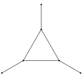
To derive the main negative result, we prove a theorem on graph coloring, which seems to be of interest on its own right, too. It statesAPX-hardness of the chromatic number on a restricted class of graphs. Interestingly enough, the corresponding result on scheduling was widely believed2 to have been proved via triangle packing; but actually there is no quantitative equation between optimal triangle packings and optimal schedules. We illustrate this fact with a simple example in Figure 1. The vertices represent unit-time jobs,
2 Section 1.2 of [17, p. 200] claims “a hardness gap for maximum packing of triangles in a graph (...) implies a hardness gap for scheduling with conflicts of unit jobs on 3 machines.”
Figure 1: Small counterexample to a suspected relation between triangle packings and optimal schedules.
and the edges represent those pairs of jobs which are processable simultane- ously. (The number of machines can be any m≥3.)
An optimal schedule requires makespan 3, by processing the two jobs of a pendant edge in each time slot. On the other hand, starting from the optimal triangle-packing and hence processing the three jobs of the central triangle at the same time, each of the remaining jobs (the three pendant vertices) require a further distinct time slot, yielding a schedule with makespan 4.
Section 2 is devoted to exact and approximation algorithms and their analysis, Section 3 gives a PTAS for the case of B = 1 with a fixed number of machines, and Section 4 contains inapproximability results. We finish in Section 5 with some conclusions and topics for future research.
1.3 Some Terminology
Given an instance of the RAR-problem, we use the term assignment if the jobs are assigned to the machines in a feasible way (i.e., the machine assign- ment restrictions are satisfied), without fixing the time slots to execute the jobs. If the jobs already got also their time slots where they are processed, this assignment is called schedule. For a set of jobs J0 ⊂ J we denote by p(J0) the total processing time of the jobs in J0, i.e., p(J0) =P
j∈J0pj. In a graphG = (V, E) with vertex set V and edge set E, a set S ⊂V is independent if any two v, w∈S are nonadjacent. Theindependence number of Gis the maximum cardinality of an independent set in G. Thechromatic number is the minimum number of independent sets whose union is the entire vertex set V. Equivalently, it is the minimum number of colors that can be assigned to the vertices in such a way that no two adjacent vertices get the same color. A clique cover of G is a collection of complete subgraphs
whose union contains all vertices of G. Throughout this paper we restrict our attention to clique covers in which the complete subgraphs are mutually vertex-disjoint.
A matching in a graph is a collection of mutually vertex-disjoint edges;
with an alternative terminology, any two edges of a matching are nonadja- cent. The matching number is the maximum number of edges in a matching.
The chromatic index of a graph or multigraph G is the minimum number of matchings whose union is the set E of all edges. Equivalently, it is the minimum number of colors that can be assigned to the edges in such a way that no two adjacent edges get the same color.
1.4 Approximation and L-Reduction
For an optimization problemP, ifI is a problem instance andz is a solution on I, we denote by OptP(I) the optimum value on I. If not stated oth- erwise, let OptRAR denote the optimal solution value for the RAR-problem and OptRA be the optimal solution for the RA-problem, respectively. Let valP(I, z) denote the actual value of solutionz; we may simply writeval(I, z) ifP is understood. GivenP and a realρ >1, an algorithm is aρ-approximation algorithm if it determines a solutionzfor every instanceI, with the property that valP(I, z)≤ ρOptP(I) if P is a minimization problem, and valP(I, z)≥
1
ρOptP(I) ifP is a maximization problem. A family ofρ-approximation algo- rithms is called apolynomial-time approximation scheme (PTAS)ifρ= 1 +ε for any ε >0 and the running time is polynomial with respect to the length of the problem input. A family of ρ-approximation algorithms is called a fully polynomial-time approximation scheme (FPTAS) if ρ = 1 +ε for any ε >0 and the running time is polynomial with respect to both the length of the problem input and 1/ε.
Consider now two NP-optimization problems, say A and B. As intro- duced in [27], an L-reduction from A to B consists of two functions f and g, computable in polynomial time, for which there exist constants α, β >0 such that:
• if I is an instance of problem A, then f(I) is an instance of problem B, satisfying
OptB(f(I))≤α·OptA(I) ;
• if z is a solution on f(I), theng(z) is a solution on I, satisfying
|OptA(I)−valA(I, g(z))| ≤β· |OptB(f(I))−valB(f(I), z)|. The problem class APX consists of those optimization problems P for which there exists a C-approximation with some constant C. The relevance of L- reduction is that if a problem A is APX-hard and there is an L-reduction form A toB then also B isAPX-hard.
2 Exact and Approximation Algorithms
In this section we will present optimal algorithms with polynomial running time for two special cases, and a polynomial approximation algorithm for the general case. For the unit-time case with B = 1 we will give an exact algo- rithm with running time in O((m3 +m2n) logn) and for the unit-time case with two machines we will give an optimal algorithm applying a maximum matching algorithm. For the general case we design a polynomial approxi- mation algorithm with worst-case bound B + 2−1/m.
Solving the problem with two machines and unit-time jobs is straightfor- ward using matching techniques.
Theorem 1. The RAR-problem with unit-time jobs and two machines can be solved in polynomial time.
Proof. We define a graphG= (V, E). The vertices inV consist of the jobs 1, . . . , n. There is an edge between vertexi and vertex j if and only if jobsi and j have no resource in common which they require, i.e., R(i)∩ R(j) =∅ and, moreover, it is not the case that |M(i)| = |M(j)| = 1 and M(i) = M(j). In this graphical representation two unit-time jobs can be processed in the same time interval if and only if they are connected by an edge. If a maximum matching of this graph has ν edges, then the minimum makespan of a feasible schedule is n−ν, and vice versa. Now the theorem follows by the fundamental result of Edmonds [16] that the matching number of graphs
can be determined in polynomial time.
The next theorem shows that for unit processing times and B = 1, the RAR-problem can be solved in polynomial time on any (maybe not even a constant) number of machines. Better bounds could be given for large m,
but the main point here is polynomiality; moreover the formula is very strong if m is small, which is the typical case in scheduling.
Theorem 2. The RAR-problem with n unit-time jobs andm machines can be solved in O((m3+m2n) logn) time for B = 1.
Proof. Let f be a given positive integer. We will present an algorithm which examines in polynomial time whether an assignment exists with finish time less than or equal to f. The optimal value of f can then be found by binary search. Set λmax = max{λ1, . . . , λµ}. Since λmax is a lower bound for the optimal finish time, we may assume that f ≥ λmax. Notice further that for B = 1, the sets Λ0,Λ1, . . . ,Λµ are disjoint and hence (Λ0,Λ1, . . . ,Λµ) is a partition of J. In the first stage, we will check whether there is a feasible assignment of jobs to machines with makespan at most f while ignoring the resource requirements. This is done by solving an appropriate network flow problem in a bipartite network N.
The network N is defined as follows. From a source node s we have arcs to all nodes of a set V1 ={1, . . . , n} of n nodes which represent the n jobs.
The second part of the node set is given by V2 ={M1, . . . , Mm}. From node j there is an arc to node Mi if and only if Mi ∈ M(j). There is an arc from each node Mi to the sink t. All arcs have capacity 1 except for the arcs incident with t, which have capacity f. Applying standard techniques including the Flow Integrality Theorem, it follows that there is a feasible assignment of jobs to machines with makespan at most f if and only if N admits a flow from s tot with flow value n.
If a flow with flow value n exists, we take such an integral flow and use the computed assignment of jobs to machines in order to assign the jobs to time slots in the second stage. We have to assure that two jobs from the same set Λk, k = 1, . . . , µ are not processed simultaneously. Since there are no restrictions for the time slots for jobs in Λµ+1, they are given into the time slots of idle time leftover after assigning the jobs from Λ1, . . . ,Λµ. For the assignment of the jobs from Λ1, . . . ,Λµ we will define a bipartite multigraph G with vertex set V =V1 ∪V2. The set V1 consists of µvertices R1, . . . , Rµ. The vertex set V2 corresponds to the m machines M1, . . . , Mm. There is an edge between vertices Rk and Mi if and only if at least one job j ∈ Λk has been assigned to Mi in the first stage. The multiplicity of the edge is equal to the number of jobs assigned to Mi from Λk.
Recall that the chromatic index of a (multi)graphGis the smallest num- ber of colors needed to partition the edge set of G into color classes so that
each class is a matching. Given such an edge coloring of G, we identify each color with a time slot; and then theλk jobs in Λk can be assigned arbitrarily to theλkdifferent time slots corresponding theλkcolors of the edges incident to Rk. It is easily seen that there is a feasible schedule of makespan f if we can find an edge coloring with at most f colors, and vice versa: “Each job requiring the same resource has to be processed in different time slots” trans- lates into “All edges incident to some vertex v ∈ V1 must receive different colors.” “At each time, each machine executes at most one job” translates into “All edges incident to some v ∈ V2 must receive different colors.” It is well-known that a bipartite graph (or multigraph) with maximum degree h has also chromatic index h (see e.g. Berge [4, p. 247]).
Sincef ≥λmax,Ghas maximum degreef, and hence the desired feasible schedule exists. To find such a schedule, we use the algorithm due to Alon for minimal edge coloring of bipartite multigraphs [2].
Let us look at the time complexity. The networkN of Stage 1 has|V1|=n and the number of arcs in N is in O(nm). Hence, the algorithm of Ahuja et al. [1] for bipartite network flows uses O(m3 +m2n) time. Since graph G has only n edges, we need O(nlogn) time for the coloring algorithm in Stage 2, see [2]. Clearly, all jobs can be finished by time n. Thus, we can find a schedule with minimum makespan using binary search with at most log(n) steps. This gives the claimed time complexity.
We investigate now the RAR-problem with arbitrary processing times.
Our approximation algorithm is again composed of two stages. In the first stage an assignment of jobs to machines with an approximation on the mini- mum finish time is given while ignoring the resources. This means that in the first stage a solution for the RA-problem is computed. In the second stage this assignment is transformed into a feasible schedule for the RAR-problem.
Let us now assume that we have found an assignment of the jobs to the machines using a heuristic H by ignoring the resources. Let Cmax(H) denote the makespan produced by heuristic H. We fix in the second stage the schedule for each machine, taking into account that jobs requiring the same resource cannot be processed simultaneously. This is done by a greedy approach as follows.
Algorithm G
Input: An assignment of jobs to machines produced by a heuristic H
Output: A heuristic schedule S
1. Let t be the first time, such that some machine Mi is available and there is a job j, that may be started by Mi at time t. Select j to be the next job processed by Mi.
2. Repeat Step 1 until all jobs are scheduled. Stop.
Let p(Λk) be the total length of all jobs which require resource Rk, i.e., p(Λk) =P
j∈Λkpj, for k = 1, . . . , µ. Set p(Λmax) = maxk=1,...,µp(Λk).
It can be easily seen that the running time of Algorithm G is at most O(mn2B). We now analyze its worst-case performance.
Theorem 3. Let Cmax(G) be the makespan of Algorithm S after applying heuristic H. Then
Cmax(G)≤Cmax(H) +p(Λmax)·B.
Proof. Let S be the schedule produced by G. Without loss of generality, suppose that machine Mm is the one which terminates schedule S. Let Q be the set of jobs processed by Mm after the last idle interval for Mm. We assume that Q is not empty, since otherwise Cmax(G) = Cmax(H) and the theorem obviously holds.
Each of the jobs of set Q requires at least one resource; otherwise a job from Λµ+1 would have started earlier. Select one of the jobsj ∈Q.It follows that the total idle time of Mm does not exceed the total time for processing all jobs that require at least one of the resources in R(j). Indeed, job j was not able to start in an idle interval because resources in R(j) were required by some other jobs in that entire interval. This means that the union of idle intervals for Mm is completely contained in the union of intervals in which jobs requiring resources from R(j) are processed. Thus, the total time of this union of intervals is bounded from above by P
k∈R(j)
p(Λk). Sinceρj ≤B, we conclude that
Cmax(G)≤Cmax(H) + X
k∈R(j)
p(Λk)≤Cmax(H) +p(Λmax)·B.
Corollary 4. If heuristicH provides anα-approximation for the RA-problem, we obtain an (α+B)-approximation algorithm for the RAR-problem.
Proof. Recall thatOptRAR denotes the optimal solution value for the RAR- problem and OptRA the optimal solution for the RA-problem, respectively.
Then, we have
OptRAR≥max{OptRA, p(Λmax)}. Using Theorem 3 we get
Cmax(S)≤α·OptRA+p(Λmax)·B ≤(α+B)·OptRAR.
Theorem 5. There is a polynomial-time(2−1/m+B)-approximation algo- rithm for the RAR-problem on m machines with arbitrary processing times.
Proof. Consider the scheduling problem of minimizing the makespan on unrelated machines, R| · |Cmax. In the unrelated machine problem, job j has processing time pij on machine i.
For an assignment of jobs to machines in the RA-problem the processing times pij reduce to
pij =
pj, i∈ M(j)
∞, otherwise.
Recall that Lenstra et al. [24] present a 2-approximation algorithm for problem R| · |Cmax. Using the improved rounding scheme of Shchepin and Vakhania [29] it is even possible to find a solution for IP with makespan
Cmax(SV)≤
2− 1 m
OptRA, (1)
where Cmax(SV) denotes the makespan obtained by applying the algorithm in [29] and OptRA corresponds to an optimal solution of the RA-problem.
Replacing α by 2−1/m in Corollary 4 we get the desired result.
Corollary 6. If B is a constant, there is a polynomial-time approximation algorithm with constant worst-case bound for the RAR-problem.
Corollary 7. There is a polynomial-time (1 +B)-approximation algorithm for the RAR-problem with unit-time jobs and abritrary number of machines.
Proof. It can be easily seen that the RA-problem with unit-time jobs is solvable in polynomial time by maximum cardinality bipartite matching.
Corollary 8. For any fixed > 0 there is a polynomial-time (1 +ε+B)- approximation algorithm for the RAR-problem, when the number of machines m is a constant.
Proof. It is well-known that there is an FPTAS for the problem Rm| · |Cmax
with a fixed number of machines.
A special case of the restricted assignment problem is the problem where the sets M(j) are nested: for any two jobs j and k, either M(j)∩ M(k) =
∅, or M(j) ⊆ M(k), or M(k) ⊆ M(j). Muratore et al. [26] derive a polynomial-time approximation scheme for the restricted assignment problem with nested constraints (without any assumptions on m). This results in the following corollary.
Corollary 9. For any fixed > 0 there is a polynomial-time (1 +ε+B)- approximation algorithm for the RAR-problem with nested constraints, even when the number of machines m is part of the input.
Proof. Replace α by 1 +ε for this special RA-problem.
3 A PTAS for a Fixed Number of Machines and B = 1
In this section we present a polynomial time approximation scheme (PTAS) for the RAR-problem with B = 1 for which the number of machines m is fixed. Our proof is an extension of the proof in [20] for the problem with parallel dedicated machines with a single resource P Dm|res111|Cmax where each job has to be processed on exactly one machine and one resource is available. For the sake of completeness, we will repeat those parts of the proof from [20] that are slightly modified but necessary for understanding.
Recall from the preceding section that Cmax(SV) denotes the makespan obtained by applying the algorithm in [29] to the RA-problem. Then, define
C = max{p(Λmax), p(J)/m, Cmax(SV)/2}.
Here, p(Λmax) and p(J)/m are obvious lower bounds for OptRAR. We con- clude for B = 1 from (1) that
C ≤OptRAR. (2)
Applying Theorem 3 with Cmax(SV) we get OptRAR ≤Cmax(SV) +p(Λmax) and thus
OptRAR≤3C. (3)
Letε >0 be a small number and set ˜ε=ε/74. We introduce the sequence of real numbers δ1, δ2, . . . such that
δt= ε˜
m3 2t
.
For each integert,t≥1, define the set of jobsJt={j ∈J |δ2tC < pj ≤δtC}. Obviously, J1, J2, . . . are mutually disjoint and their union isJ. Thus, there is a positive integer t0 ≤ dmε˜e such that p(Jt0) ≤ εp(J˜ )/m ≤ εC˜ holds.
Choose δ=δt0. Partition the set J of jobs into the set of big jobs J1, the set of medium jobs J2, and the set ofsmall jobs J3, defined as follows:
J1 = {j |δC < pj},
J2 = {j |δ2C < pj ≤δC}, (4) J3 = {j |pj ≤δ2C}.
The corresponding cardinalities of J1,J2, J3 are given by n1,n2, n3, respec- tively. Note that by definition J2 =Jt0, so that
p(J2)≤ε˜OptRAR. (5)
Besides,
˜ ε
m3 ≥δ≥ ε˜
m3 2dmε˜e
. (6)
We get from (3) that
n1 < 3
δ m. (7)
Consider the set ofrestricted schedules SR which consists of all the sched- ules, in which the starting times of the big jobs are non-negative integer multiples of δ2C. LetOptSR denote the optimal solution value for the RAR- problem restricted to classSR. Assume that the schedules are represented by Gantt-charts where the horizontal axis corresponds to the time. We trans- form an optimal schedule S∗ of the RAR-problem into a schedule SR ∈ SR by shifting jobs iteratively to the right, beginning with the smallest starting
time of a big job which is not equal to a multiple of δ2C. In each iteration jobs are shifted to the right by at mostδ2C and aftern1 iterations we obtain a schedule of class SR. Using (3) and (7) we get
OptSR ≤OptRAR+ 3mδC ≤3C(1 +mδ). (8) For the jobs of set J1, define SB as the class of schedules which con- tains all possible schedules of big jobs with starting and completion times in [0; 3C(1 +mδ)] such that all starting times are non-negative integer multi- ples of δ2C. Consider an arbitrary schedule SB ∈ SB. Let τ1 < τ2 < . . . < τq be the increasing sequence of all positive distinct starting and completion times of the big jobs. By (7) we have
q < 6
δm. (9)
For schedule SB, define the following sequence of time intervals
I0 = [0;τ1], I1 = [τ1;τ2], . . . , Ih = [τh;τh+1], . . . , Iq−1 = [τq−1;τq], Iq= [τq;∞[.
Clearly, inside a time interval Ih, 0 ≤h≤ q, no big job starts or completes.
With τq+1 =∞ and τ0 = 0 denote the length of Ih by `(Ih) = τh+1−τh for h= 0, . . . , q−1 and `(Iq) =∞.
When a time intervalIh is associated with a machineMi we denote it by Ii,h and define itscapacity by
c(Ii,h) =
`(Ih), if no big job is processed on Mi in interval Ih 0, otherwise.
The capacity for resource Rk of interval Ih is given as rk(Ih) =
`(Ih), if no big job of Λk is processed in interval Ih 0, otherwise.
The value rk(Ih) specifies the maximum total processing time of small or medium jobs in Λkwhich can be processed during time interval Ih. As in the proof of Theorem 5 the processing times pij reduce to
pij =
pj, i∈ M(j)
∞, otherwise.
We want to assign the small jobspreemptively into scheduleSB. For this purpose the linear program LP(SB) is defined as follows:
minimize z
s.t. X
j∈J3
x(i,h),jpi,j ≤c(Ii,h), i= 1, . . . , m, h= 0, . . . , q−1, (10)
m
X
i=1
X
j∈Λk
x(i,h),jpi,j ≤rk(Ih), k = 1, . . . , µ, h= 0, . . . , q−1, (11) X
j∈J3
x(i,q),jpi,j ≤z, i= 1, . . . , m, (12)
m
X
i=1
X
j∈Λk
x(i,q),jpi,j ≤z, k= 1, . . . , µ, (13)
q
X
h=0 m
X
i=1
x(i,h),j = 1, j ∈J3, (14)
x(i,h),j ≥0.
The variablex(i,h),j determines the rate of small job j which is processed in interval Ih on machine Mi. Hence, (14) guarantees that job j is fully distributed among the machines and that 0 ≤ x(i,h),j ≤ 1. Inequalities (10) ensure that the total processing time of small jobs executed in interval Ih on machine Mi does not exceed the interval length `(Ih). Inequalities (11) guarantee that the total processing time of jobs in Λk executed in intervalIh does not exceed`(Ih). By (12) and (13) the optimal objective function value z is not smaller than the maximum of the total processing time of small jobs processed on a machine after time τq and the maximum of the total processing time of small jobs which require a certain resource. Notice that LP(SB) only assigns small jobs to time intervals, but no starting times of the jobs are given and a preempted job can be assigned to different machines.
The linear program LP(SB) consists of m(q+ 1) inequalities (10), (12), µ(q+ 1) inequalities (11), (13) and n3 equations (14). Let an optimal basic
solution of LP(SB) with optimal solution valuez∗ be represented as a matrix Γ = γ(i,h),j
, i= 1, . . . , m, h= 0, . . . , q, j∈J3.
The rows of Γ correspond to all possible pairs (i, h) taken in any order, the n3 columns correspond to different small jobs. The values v1 and v2 denote the number of inequality constraints (10), (12) and (11), (13), respectively, which are satisfied as equalities by Γ. By elementary linear programming theory, the number γ+ of strictly positive values in Γ is at most n3+v1+v2. Clearly,v1 ≤m(q+ 1). For µ≤m, we havev2 ≤m(q+ 1) as well. If µ > m, then for each h, 0 ≤ h ≤ q, inequalities (11) and (13) hold as equality for at most m resource values k. We conclude that at most m(q+ 1) inequality constraints (11), (13) are non-redundant. Thus, we have shown that
γ+≤n3+ 2m(q+ 1). (15)
Call positive solution valuesγ(i,h),j withγ(i,h),j <1split values; otherwise, call positive solution values with γ(i,h),j = 1 non-split values. Notice that if γ(i,h),j is a non-split value, then jobjis completely assigned to time intervalIh on machineMi. Partition the set of small jobsJ3 into the setJ3sofsmall split jobs, i.e., those jobs j for which there is a row (i, h) such that 0 < γ(i,h),j <1, and into the set J3ns of small non-split jobs, i.e. those jobsj for which there is a row (i, h) such that γ(i,h),j = 1.
Since each job is processed on at least one machine and in at least one time interval, it follows that each of the n3 columns of matrix Γ has at least one positive entry. By (15) there are at most 2m(q+ 1) columns with more than one positive entry, and the positive entries of each such column correspond to the split values of Γ. Hence, there are at most 4m(q+ 1) split values and at most 2m(q+ 1) small split jobs. Since the maximum processing time of a small split job is δ2C, we obtain
p(J3s)≤2m(q+ 1)δ2C. (16) Temporarily, ignore the setJ3s. For each time intervalIhwe define an open shop problem where the small non-split jobs which use the same resource and are assigned to Ih byLP(SB) form an operation. The schedule of each such open shop problem corresponds to time slots to which we assign the original jobs afterwards. More precisely, let J(i,h),Λk denote the set of small non-split
jobs which require resource k and which are assigned byLP(SB) to machine Mi in time interval Ih, i.e.,
J(i,h),Λk =
j ∈J3ns| j ∈Λk, γ(i,h),j = 1 i= 1, . . . , m, h= 0, . . . , q, k= 1, . . . , µ.
Analogously,
J(i,h),Λ0 =
j ∈J3ns| j ∈Λ0, γ(i,h),j = 1
is the set of small non-split jobs which require no resource and which are assigned byLP(SB) to machineMi in time intervalIh. Then, define for each time interval Ih, h = 0, . . . , q, an open shop problem OS(h) on m machines with m+µ jobs as follows. There are given µ jobs Oh,k, k = 1, . . . , µ, with operations O(i,h),k on machine Mi, i = 1, . . . , m. These operations have the processing times
p(O(i,h),k) = X
j∈J(i,h),Λ
k
pj, i= 1, . . . , m, k= 1, . . . , µ. (17) Furthermore, there are m jobs O(i,h),0, i = 1, . . . , m, which consist of single operations, also denoted as O(i,h),0, which have to be processed on machine Mi. They have the processing times
p(O(i,h),0) = X
j∈J(i,h),Λ0
pj, i= 1, . . . , m. (18) Each job Oh,k of problem OS(h), h = 0, . . . q, has release time τh. We allow the jobs to be preemptive. Hence, the problem can be classified in 3-field notation as Om|pmtn|Cmax. LetOptOS(h) denote the optimal solution of problem OS(h).
For a classic open shop problem onmmachines withnjobs and operation times qij, i = 1, . . . , m, j = 1, . . . n, there are two obvious lower bound on the optimal makespan:
LB1 = max ( n
X
j=1
qij | i= 1, . . . , m )
(machine based lower bound),
and
LB2 = max ( m
X
i=1
qij | j = 1, . . . , n )
(job based lower bound).
If the open shop problem is preemptive, there is a polynomial algorithm which finds an optimal schedule with solution value equal to max{LB1, LB2} (see [28] for details). Inequalities (10) and (11) imply that
OptOS(h)≤τh+1, h= 0, . . . , q−1. (19)
Analogously, inequalities (12) and (13) correspond to the machine based and the job based lower bound, respectively. This implies that
OptOS(q) ≤τq+z∗. (20)
Notice that there is an optimal schedule forOm|pmtn|Cmaxthat has no more than 4m2 preemptions. A possible algorithm for finding such a schedule is described in [23].
Consider such an optimal schedule for problem OS(h), h= 0, . . . , q. For each k, k = 0, . . . , µ, and each machine Mi, i = 1, . . . , m, identify the se- quence T(i,h),ku , u = 1,2, . . . , of time slots in which the operation O(i,h),k is processed (preemptively) on machine Mi. For each such interval T(i,h),ku de- termine its length `(T(i,h),ku ). Notice that,
p(O(i,h),k) = X
u
` T(i,h),ku
. (21)
We are now able to formulate the PTAS for our problem.
Algorithm RARm
Input: An instance of the RAR-problem with B = 1, a fixed number of machines m and accuracy ε >0
Output: A heuristic schedule Sε
1. For a given ε, determine ˜ε and δ. Partition the set J of jobs into the subsets J1, J2 and J3 of big, medium and small jobs, respectively, as defined in (4).
2. For each schedule SB ∈ SB solve the corresponding linear program LP(SB) and find the optimal valuez∗of the objective function. Identify schedule SB∗ ∈ SB for which the value z∗ +τq attains its minimum.
Denote Iq+1 = [τq;τq+z∗].
3. For the scheduleSB∗ solve the correspondingq+ 1 open shop problems OS(0), OS(1), . . . , OS(q) such that each optimal solution has at most 4m2 preemptions. For each i = 1, . . . , m, h = 0, . . . , q, k = 0, . . . , µ, assign the jobs in J(i,h),Λk non-preemptively to the corresponding time- slots T(i,h),ku , u = 1,2, . . . , by using First Fit. The small non-split jobs which could not be sequenced are collected in set J3ns1.
4. The jobs which are not assigned yet, i.e., the medium jobs J2, small split jobs in J3s and the small non-split jobs in J3ns1, are sequenced at the end of the schedule in any order. We obtain schedule Sε with makespan Cmax(Sε).
Theorem 10. Algorithm RARm is a PTAS for the RAR-problem with a fixed number of machines and B = 1.
Proof. Algorithm RARmruns in polynomial time for fixed m and ε. This is guaranteed by the fact that the maximum number of schedules in SB is in O((mδ2)3mδ ) and is therefore a constant. We prove that the algorithm produces a schedule with makespan not greater than (1 +ε)OptRAR.
The optimal solution of LP(SB∗) gives a lower bound for the optimal solution values of schedules in SR, i.e.,
z∗+τq ≤OptSR. (22)
Inequalities (19), (20) guarantee that the time-slots produced in Step 3 fit into the intervals I0, I1, . . . , Iq+1. Therefore, the small jobs assigned in Step 3 are finished before τq+z∗ and the makespan of schedule Sε is bounded by the total processing time of the jobs assigned in Step 4 plus τq+z∗, i.e.,
Cmax(Sε)≤τq+z∗+p(J2) +p(J3s) +p J3ns1
. (23)
The total processing time of the medium jobs and the small split jobs is bounded by (5) and (16). We have to estimate the number of small non-split jobs that cannot be scheduled in Step 3 of the algorithm. Therefore, we turn to the time slots T(i,h),ku introduced in Step 3 of Algorithm RARm. Collect the time slots T(i,h),ku which correspond to the same operation in set ˆT(i,h),k, i.e.,
Tˆ(i,h),k =
T(i,h),ku |u= 1,2, . . . .
First, consider the time slots which belong to one-element sets ˆT(i,h),k. From (17), (18) and (21) follows that in Step 3 of the algorithm all jobs of J(i,h),Λk are processed on machine Mi as a single block.
Collect the time slots which belong to sets ˆT(i,h),k with more than one element, in set ˆT1 and define t1 = |Tˆ1|. Recall that there are at most 4m2 preemptions for each open shop problemOS(h),h= 0, . . . , q. Any set ˆT(i,h),k with v elements (v ≥ 1) corresponds to v −1 preemptions in interval Ih. Hence, we get t1 ≤8m2(q+ 1) and at most 8m2(q+ 1) small non-split jobs cannot be assigned by First Fit in Step 3. This results in
p J3ns1
≤8m2(q+ 1)δ2C. (24)
Now it is possible to estimateCmax(Sε) by inserting (5), (16) and (24) in (23). We get
Cmax(Sε)≤τq+z∗+ ˜εOptRAR+ 2m(q+ 1)δ2C+ 8m2(q+ 1)δ2C. (25) Applying (2), (8) and (22) inequality (25) simplifies to
Cmax(Sε)≤ 1 + 3mδ+ ˜ε+ 2m(q+ 1)δ2+ 8m2(q+ 1)δ2
OptRAR.
Inserting (9) and afterwards (6) we deduce
Cmax(Sε) ≤ 1 + 3mδ+ ˜ε+ 12m2δ+ 2mδ2+ 48m3δ+ 8m2δ2
OptRAR
≤
1 + 3˜ε
m2 + ˜ε+ 12˜ε m + 2˜ε2
m5 + 48˜ε+8˜ε2 m4
OptRAR
≤ (1 + 74˜ε)OptRAR
= (1 +ε)OptRAR.
Thus, we have shown that Algorithm RARm is a PTAS. The theorem is
proved.
4 Inapproximability for Unit-Time Jobs
In this section we study the RAR-problem for unit-time jobs, but with no upper bound on B. We first show that this subproblem cannot be approx- imated within any constant bound. Then, by studying graph coloring on
a restricted class, we will prove that even the problem with unit-time jobs and just three machines is APX-hard. Notice that for the unrelated machine problem with any fixed number of machines, namelyRm| · |Cmax, an FPTAS can be constructed by using standard dynamic programming techniques (see e.g. [19]).
Let us note further that the RAR-problem with any fixed number m of machines and arbitrary processing times is in APX, because a trivial m- approximation is to schedule all jobs sequentially (each job j on any ma- chine chosen from M(j)). Hence, if m is bounded, APX-hardness and APX- completeness are equivalent. For unbounded m, however, approximation is much less efficient, as shown in the following result. It extends the corre- sponding observation from [17, p. 209] to a stronger form allowed by the current model; it is adjusted from [13, Theorem 11] to the RAR terminology.
Theorem 11. The RAR-problem cannot be approximated within O(n1−) for any fixed >0 in polynomial time, unless P =NP, even when restricted to instances where all jobs have unit time, each job can be processed on exactly one machine, each machine processes exactly one job, and each resource is required by at most two jobs.
Proof. We recall a reduction from [13], where it was constructed for a more general problem, but works also for the current restricted one, too, without modification. We apply the theorem of Zuckerman [31], which states that the chromatic number of graphs does not admit a polynomial-time O(n1−)- approximation for any > 0, where n is the number of vertices. So, let G = (V, E) be a graph of order n, and denote its vertices by v1, . . . , vn. Each vi corresponds to a unit-time job i. We assume here m =n, and that machineMi is dedicated to process jobi. In this way the machines can work independently at any time, except that restrictions will be created by the resource requirements.
We define µ = |E|, and index the resources with the edges of G. If vivj ∈ E, then there is a resource Rij required for both jobs i and j (but not for any other job). This ensures that iand j cannot be processed at the same time.
Since there are no more restrictions, it follows that a subsetS ⊂ {1, . . . , n} of jobs can be processed simultaneously in the same time slot if and only if the set {vi | i ∈ S} is independent in G. Thus, minimum makespan equals
the chromatic number of G.
The scheduling problem for parallel dedicated machines under resource constraints, briefly P D|resµ11|Cmax, is a special case of the RAR-problem where each job has to be processed on exactly one machine. It was shown in [21] that there is a PTAS for this problem when the number of machines is a constant. In contrast, Theorem 11 shows that even for unit-time jobs it is non-approximable with a constant worst-case bound when the number of machines is part of the input.
Corollary 12. The scheduling problem P D|resµ11|Cmax cannot be approxi- mated within O(n1−) for any fixed > 0 in polynomial time even for unit- time jobs, unless P = NP.
It should be noted that the problem instances constructed in the proof above have input sizes of order n2. Currently we do not know what kind of lower bound holds for instances whose size grows more slowly, e.g. is linear in n.
As the main tool for theAPX-hardness result, next we prove a theorem on graph colorings and clique covers, which is of interest on its own right, too.
The algorithmic problems Chromatic Number and Minimum Clique Cover take a graph G as input, and ask for the chromatic number of G and the minimum number of complete subgraphs3 in a clique cover of G, respectively. Although there is an extensive literature on the approximability of the chromatic number of graphs, we were not able to find the theorem given below.
Theorem 13. The following optimization problems are APX-complete:
(i) the Chromatic Numberproblem restricted to graphs of independence number 3,
(ii) the Minimum Clique Coverproblem restricted to graphs whose clique number is 3,
(iii) even more restrictively the Minimum Clique Coverproblem on graphs whose clique number is 3 and maximum degree is 4.
3 Since all induced subgraphs of a complete graph are complete, the minimum is the same independently of whether it is assumed that the subgraphs used in the cover are vertex-disjoint.
Proof. Membership in APX is immediately seen, because the optimum clearly is at most n and at least n/3 for every graph of order n; thus, the solution ‘n’ is a trivial 3-approximation. Also, equivalence between (i) and (ii) holds by taking complementary graphs. For this reason it suffices to prove that there is no PTAS for Minimum Clique Cover under the degree-4 condition, unless P=NP.
We apply L-reduction from the Max-2-SAT-3 problem, which is APX- hard by the theorem of Berman and Karpinski [5]. (More explicitly, ifP6=NP, then it is not possible to approximate the optimum within a multiplicative 1.0005 in polynomial time.) The construction below is quite similar to the one given by Caprara and Rizzi [11] for the problem of determining the maxi- mum number of vertex-disjoint triangles in graphs,4 but there are substantial differences: the current structure is somewhat simpler, but nevertheless its verification is much more tedious.
Let Φ be a Boolean formula over thenvariablesx1, . . . , xnwithmclauses c1, . . . , cm such that each clause is either a single literal or the disjunction of two literals, and each variable occurs in at most three clauses (where both literals xi and ¬xi are counted). The task is to maximize the number of satisfied clauses in a truth assignment. Note that
Opt(Φ) ≥m/2
because the all-true and all-false assignments together satisfy each clause, therefore one of them satisfies at least half of the clauses.
We may assume without loss of generality that each variablexi occurs in at least one positive and also in at least one negative literal, for otherwise we can set all clauses containing xi true, hence reducing the instance to a smaller one in constant time. Thus the total number of literals is at least 2n;
but it cannot exceed 2m (by the condition on clause size), therefore m ≥ n holds, which implies
Opt(Φ) ≥n/2.
For the sake of simpler formalism it is also convenient to assume that if a variable occurs in three clauses, then two of those literals are positive and one is negative. (In the opposite case just switch between positive and
4 Note that a clique cover may use not only triangles and vertices but also edges, moreover there is no guarantee that an optimal solution occurs where the number of triangles is maximum.
negative for this variable in the clauses and also betweentrue and falsein its truth assignment.)
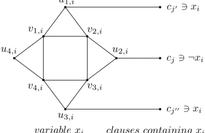
From every instance Φ satisfying the restrictions above, we construct a graph GΦ on 8n+m vertices, which will be an instance of the problem in (iii); cf. Figure 2. Itsmclause-vertices will simply be denoted byc1, . . . , cm.
c
j003 x
ic
j03 x
ic
j3 ¬ x
iclauses containing x
ior ¬ x
ivariable x
iFigure 2: Variable gadget forxi, and its adjacencies to clause vertices The variable-gadgets have eight vertices each: the gadget belonging to xi has vertex set {u1,i, u2,i, u3,i, u4,i, v1,i, v2,i, v3,i, v4,i}. The central part of the gadget is a 4-cycle C(i) = v1,iv2,iv3,iv4,i, its vertices appear along the cycle in this order; and the other four vertices are the third vertices of four triangles:
T1,i =u1,iv1,iv2,i, T2,i=u2,iv2,iv3,i, T3,i=u3,iv3,iv4,i, T4,i=u4,iv4,iv1,i. If cj is the (unique) clause where ¬xi appears as a negative literal, then there is an edge cju2,i; and if cj0, cj00 are the two clauses where xi appears as a positive literal (say, j0 < j00), then there are two edges cj0u1,i and cj00u3,i. Should xi as a positive literal occur in just one clause cj0, only cj0 will be adjacent withu1,i, henceu3,i has then degree 2 inGΦ. One can constructGΦ
from Φ in linear time. Moreover, we clearly have Opt(GΦ)≤4n+m≤10·Opt(Φ)
(where 10·Opt(Φ) is a very rough upper bound, but the actual coefficient of Opt(Φ) is irrelevant with respect to L-reduction).
Claim. For any clique cover K of GΦ there exists a clique cover K∗ such that |K∗| ≤ |K| and, for each index i (1 ≤ i ≤ n), either T1,i, T3,i ∈ K∗ or T2,i, T4,i ∈ K∗.
The proof of this claim is easy but somewhat tedious since one has to consider quite a few cases. It proceeds by making local modifications inside each variable gadget. To perform them, it suffices to concentrate on those cliquesK ∈ K, termedcrossing clique, which contain vertices both inside and outside the central 4-cycle C(i) of the gadget in question. Note that such cliques do not have any clause vertices, and contain precisely one neighbor u`,i of C(i). We make primary distinction by inspecting the positions of the intersections
K∩ {v1,i, v2,i, v3,i, v4,i},
with secondary distinction by the vertex of K in{u1,i, u2,i, u3,i} if literals of xi appear in precisely three clauses, or in {u1,i, u2,i} if each of xi and ¬xi
appears in precisely one clause.
A systematic listing of cases is given in the Appendix. As an example for the transformation, suppose thatK ={u1,i, v2,i}is the unique such clique. It means thatu2,i andu3,i are contained in some “external” cliques, sayK2 and K3, which do not meetC(i); but some cliques ofKmust containu4,i,v1,i,v3,i, and v4,i. This needs at least two cliques of K not yet listed. We then omit those two cliques from K, and do the following further local modifications:
adjoin v1,itoK, which yieldsT1,i; remove u3,i fromK3, and cover it together withv3,i andv4,i asT3,i; and take the singleton{u4,i}as an additional clique.
In this way two cliques of K have been removed and two others inserted, while all vertices are still covered and {T1,i, T3,i} is included in the modified cover. (The clique K2 remained unchanged.) The other situations can also be handled with similar modifications, some of them leading to |K∗| <|K|, some others keeping |K∗|=|K| similarly to the present one.
We now define a mapping from the set of solutions onGΦ to set of solu- tions on Φ, specifying a truth assignmentfK(xi) for each clique coverK. For i= 1, . . . , nlet
fK(xi) =
true if {T2,i, T4,i} ⊂ K∗, false if {T1,i, T3,i} ⊂ K∗.
Observe the following fact: If an xi is a positive literal in a clause cj, and in the variable gadget of xi the clique cover K∗ uses the triangles T2,i and T4,i,
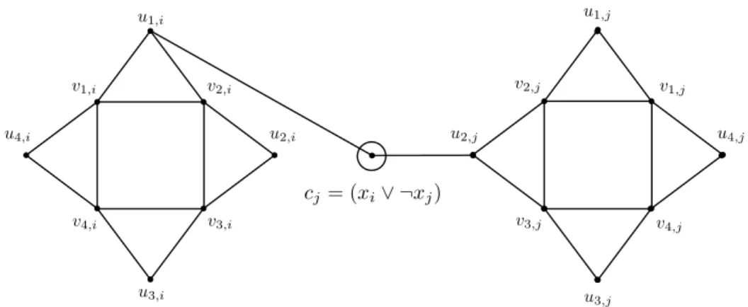
then the value of cj is set true by fK. A similar relation holds for negative literals in connection with T1,i and T3,i. Thus, if fK(cj) = false, then K∗ contains {cj} as a separate clique (cf. Figure 3), therefore
cj = (xi_ ¬xj)
Figure 3: Non-satisfied clause yields singleton clique
val(GΦ,K)≥val(GΦ,K∗)≥4n+m−val(Φ, fK). (26) We can define a mapping in the opposite direction, too. If f is a truth assignment in which the set of satisfied clauses is {cj | j ∈ Jf} (where Jf ⊆ {1, . . . , m}), then a clique cover Kf can be generated by the following rules:
• if f(xi) =true, then put T2,i and T4,i intoKf;
• if f(xi) =false, then put T1,i and T3,i intoKf;
• for eachj ∈Jf select an indexij such that the literal ofxij sets cj true;
• put the edge cju`,ij into Kf, where u`,ij is the neighbor of cj in the vertex gadget of xij;
• each vertex not covered so far is put into Kf as a complete subgraph of order 1.
Since the set
{u`,i|1≤i≤n, 1≤`≤4}
is independent, every clique cover of the subgraph induced by the variable gadgets contains at least 4n complete subgraphs. The cover Kf uses fur- ther complete subgraphs only for those clauses which are not satisfied by f.
Applying this to an optimal truth assignment, we obtain:
Opt(GΦ)≤4n+m−Opt(Φ). (27) The combination of the inequalities (26) and (27) yields
Opt(Φ) +Opt(GΦ)≤4n+m≤val(Φ, fK) +val(GΦ,K), thus the inequality
|Opt(Φ)−val(Φ, fK)| ≤ |Opt(GΦ)−val(GΦ,K)|
is valid for every solution K on GΦ. It implies that we have an L-reduction, and consequently the problems listed in (i)–(iii) are APX-hard.
Theorem 14. The RAR-problem is APX-complete, even when it is restricted to the following type of instances: there are only three machines (m = 3), all jobs have unit time (pj = 1 for all 1≤ j ≤ n), any job can be processed on any machine (M(j) = {M1, M2, M3} for all 1≤j ≤n), and each resource is required only for two jobs (|Λk|= 2 for all 1≤k≤µ).
Proof. We apply Theorem 13(i), constructing a reduction from theChro- matic Number problem. Let G be a graph in which no four vertices are mutually nonadjacent. Let the vertices v1, . . . , vn of G represent unit-time jobs 1, . . . , n, and let each edge vivj ∈ E(G) mean that there is a resource R(i, j) required for precisely the jobs i and j. If vi and vj are nonadjacent, then there is no such common resource for them. Suppose further that any of the three machines M1, M2, M3 can process any of the jobs 1, . . . , n. Then a subset of jobs can be scheduled within a unit time slot if and only if the corresponding vertices are mutually nonadjacent. Thus, the optimum make- span for the RAR-problem instance is equal to the chromatic number of G.
Consequently, the problem is APX-hard. Since membership in APX is clear
(as noted above), the theorem follows.
Corollary 15. The SWC-problem is APX-hard on three machines with unit- time jobs.