1Introduction AMultivariateComplexityAnalysisoftheMaterialConsumptionSchedulingProblem

(1)

A Multivariate Complexity Analysis

of the Material Consumption Scheduling Problem

^∗

Matthias Bentert,¹ Robert Bredereck,^{1, 2} P´eter Gy¨orgyi,³ Andrzej Kaczmarczyk,¹ and Rolf Niedermeier¹

1 Technische Universit¨at Berlin, Faculty IV,

Algorithmics and Computational Complexity, Berlin, Germany {matthias.bentert, a.kaczmarczyk, rolf.niedermeier}@tu-berlin.de

2 Humboldt-Universit¨at zu Berlin, Institut f¨ur Informatik, Algorithm Engineering, Berlin, Germany robert.bredereck@hu-berlin.de

3 Institute for Computer Science and Control, Eötvös Loránd Research Network, Budapest, Hungary gyorgyi.peter@sztaki.hu

March 15, 2021

Abstract

The NP-hard Material Consumption Scheduling Problemand related problems have been thoroughly studied since the 1980’s. Roughly speaking, the problem deals with minimizing the makespan when scheduling jobs that consume non-renewable resources. We focus on the single-machine case without preemption: from time to time, the resources of the machine are (partially) replenished, thus allowing for meeting a necessary precondition for processing further jobs, each of which having individual resource demands. We initiate a systematic exploration of the parameterized computational complexity landscape of the problem, providing parameterized tractability as well as intractability results. Doing so, we mainly investigate how parameters related to the resource supplies influence the problem’s computational complexity. This leads to a deepened understanding of this fundamental scheduling problem.

Keywords. non-renewable resources, makespan minimization, parameterized computational complexity, fine-grained complexity, exact algorithms

1 Introduction

Consider the following motivating example. Every day, an agent works for a number of clients, all of equal importance. The clients, one-to-one corresponding to jobs, each time request a service having individual processing time and individual consumption of a non-renewable resource; examples for such resources include raw material, energy, and money. The goal is to

∗An extended abstract of this work appears in the Proceedings of the 35th AAAI Conference on Artificial Intelligence, AAAI’21. This full version contains additional results for multiple resources as well as full proof details.

arXiv:2102.13642v2 [cs.GT] 12 Mar 2021

(2)

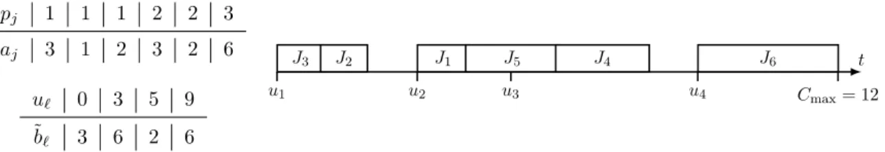
pj 1 1 1 2 2 3

aj 3 1 2 3 2 6

u` 0 3 5 9

˜b` 3 6 2 6

t

u1 u2 u3 u4 Cmax= 12

J3 J2 J1 J5 J4 J6

Figure 1: An example (left) with one resource type and a solution (right) with makespan 12.

The processing times and the resource requirements are in the first table, while the supply dates and the supplied quantities are in the second. Note thatJ₃ andJ₂ consume all of the resources supplied atu1= 0, thus we have to wait for the next supply to schedule further jobs.

finish all jobs as early as possible, known as minimizing the makespan in the scheduling literature. Unfortunately, the agent only has a limited initial supply of the resource which is to be renewed (with potentially different amounts) at known points of time during the day. Since the job characteristics (resource consumption, job length) and the resource delivery characteristics (delivery amount, point of time) are known in advance, the objective thus is to find a feasible job schedule minimizing the makespan. Notably, jobs cannot be preempted and only one at a time can be executed. Figure 1 provides a concrete numerical example with six jobs having varying job lengths and resource requirements.

The described problem setting is known as minimizing the makespan on a single machine with non-renewable resources. More specifically, we study the single-machine variant of the NP-hardMaterial Consumption Scheduling Problem. Formally, we study the following problem.

Material Consumption Scheduling Problem

Input: A setR of resources, a setJ ={J₁, . . . , J_n}of jobs each job J_j with a processing time p_j ∈ Z+ and a resource requirement a_ij ∈ Z+ from resource i ∈ R, and a set{u₁, u2, . . . , uq}of points of time with 0 =u1< u2<· · ·< uq, where ˜bi,` quantities of resourcei∈ R are supplied.

Task: Find aschedule σ with minimum makespan for a single machine without preemption which is feasible, that is, (i) the jobs do not overlap in time, and (ii) at any point of timet the total supply from each resource is at least the total request of the jobs starting untilt.

The objective is to minimize the makespan, that is, the maximum time that a job is com- pleted. Formally, the makespan is defined by C_max := maxj∈J C_j, where C_j is the completion time of jobJ_j. Notably, in our example in Figure 1 we considered the special but perhaps most prominent case of just one type of resource. In this case we simply drop the indices corresponding to the single resource. In the remainder of the paper, we make the following simplifying assumptions guaranteeing sanity of the instances and filtering out trivial cases.

Assumption 1. Without loss of generality, we assume that 1. there are enough resources supplied to process all jobs: Pq

`=1˜b_` ≥P

j∈J aj; 2. each job has at least one non-zero resource requirement: ∀_j∈JP

i∈Rai,j>0; and 3. at least one resource unit is supplied at time 0: P

i∈R˜bi,0 >0.

(3)

Note that each of these assumptions can be verified in linear time. It is valid to make these assumptions because of the following. If the first assumption does not hold, then there is no feasible schedule. If the second assumption does not hold, then we can schedule all jobs without resource requirements in the beginning. Thus, we can remove these jobs from the instance and adjust the supply times of new resources accordingly. If the third assumption does not hold (but the second does), then we cannot schedule any job before the first resource supply. Thus, we can adjust the supply time of each resource requirement such that there is a resource supply at time 0 and get an equivalent instance.

It is known that the Material Consumption Scheduling Problem is NP-hard even in the case of just one machine, only two supply dates (q = 2), and if the processing time of each job is the same as its resource requirement, that is, p_j = a_j for each j ∈ J [9]. While many variants of the Material Consumption Scheduling Problem have been studied in the literature in terms of heuristics, polynomial-time approximation algorithms, or the detection of polynomial-time solvable special cases, we are not aware of any previous systematic studies concerning a multivariate complexity analysis. In other words, we study, seemingly for the first time, several natural problem-specific parameters and investigate how they influence the computational complexity of the problem. Doing so, we prove both parameterized hardness as well as fixed-parameter tractability results for this NP-hard problem.

Related Work. Over the years, performing multivariate, parameterized complexity studies for fundamental scheduling problems became more and more popular [2, 4, 5, 6, 7, 19, 16, 29, 30, 31, 33, 32, 37, 40, 41]. We contribute to this field by a seemingly first-time exploration of the Material Consumption Scheduling Problem, focusing on one machine and the minimization of the makespan.

The problem was introduced in the 1980’s [9, 43]. Indeed, even a bit earlier a problem where the jobs required non-renewable resources, but without any machine environment, was studied [10]. There are several real-world applications, for instance, in the continuous casting stage of steel production [34], in managing deliveries by large-scale distributors [1], or in shoe production [11].

Carlier [9] proved several complexity results for different variants in the single-machine case, while Slowinski [43] studied the parallel machine variant of the problem with preemp- tive jobs. Previous theoretical results mainly concentrate on the computational complexity and polynomial-time approximability of different variants; in this literature review we mainly focus on the most important results for the single-machine case and minimizing makespan as the objective. We remark that there are several recent results for variants with other objective functions [3, 27, 28], with a more complex machine environment [26], and with slightly different resource constraints [14].

Toker et al. [44] proved that the variant where the jobs require one non-renewable resource reduces to the 2-Machine Flow Shop Problem provided that the single non-renewable resource has a unit supply in every time period. Later, Xie [45] generalized this result to multiple resources. Grigoriev et al. [21] showed that the variant with unit processing times and two resources is NP-hard, and they also provided several polynomial-time 2-approximation algorithms for the general problem. There is also a polynomial-time approximation scheme (PTAS) for the variant with one resource and a constant number of supply dates and a fully polynomial-time approximation scheme (FPTAS) for the case with q = 2 supply dates and one non-renewable resource [23]. Gy¨orgyi and Kis [24] presented approximation-preserving reductions between

(4)

problem variants with q = 2 and variants of the Multidimensional Knapsack Problem. These reductions have several consequences, for example, it was shown that the problem is NP- hard if there are two resources, two supply dates, and each job has a unit processing time, or that there is no FPTAS for the problem with two non-renewable resources andq = 2 supply dates, unless P = NP. Finally, there are three further results [25]: (i) a PTAS for the variant where the number of resources and the number of supply dates are constants; (ii) a PTAS for the variant with only one resource and an arbitrary number of supply dates if the resource requirements are proportional to job processing times; and (iii) an APX-hardness when the number of resources is part of the input.

Preliminaries and Notation. We use the standard three-field α|β|γ-notation [20], where α denotes the machine environment, β the further constraints like additional resources, and γ the objective function. We always consider a single machine, that is, there is a 1 in theα field.

The non-renewable resources are described by nr in theβ field and nr =r means that there are r different resource types. In our work, the only considered objective is the makespan Cmax. The Material Consumption Scheduling Problem variant with a single machine, single resource type, and with the makespan as the objective is then expressed as 1|nr = 1|C_max. Sometimes, we also consider the so-callednon-idling scheduling (introduced by Chr´etienne [12]), indicated by NI in theαfield, in which a machine can only process all jobs continuously, without intermediate idling. As we make the simplifying assumption that the machine has to start processing jobs at time 0, we drop the optimization goalCmax whenever considering non-idling scheduling. When there is just one resource (nr = 1), then we write aj instead ofa1,j and ˜bj

instead of ˜b_1,j, etc. We also write p_j = 1 or p_j = ca_j whenever, respectively, jobs have solely unit processing times or the resource requirements are proportional to the job processing times.

Finally, we use “unary” to indicate that all numbers in an instance are encoded in unary. Thus, for example, 1,NI|p_j = 1,unary|− denotes a single non-idling machine, unit-processing-time jobs and the unary encoding of all numbers. We summarize the notation of the parameters that we consider in the following table.

n number of jobs

q number of supply dates j job index

` index of a supply pj processing time of jobj

a_i,j resource requirement of jobj from resourcei u_` the`^th supply date

˜bi,` quantity supplied from resourceiatu`

b_i,` total resource supply from resourcei over the first`supplies, that is,P_`

k=1˜b_i,k

To simplify matters, we introduce the shorthands amax, bmax, and pmax for maxj∈J,i∈Raij, max`∈{1,...,q},i∈R˜b_i,`, and maxj∈J pj, respectively.

Primer on Multivariate Complexity. To analyze the parameterized complexity [13, 15, 17, 42] of theMaterial Consumption Scheduling Problem, we declare some part of the input theparameter (e.g., the number of supply dates). A parameterized problem is fixed-parameter tractable if it is in the classFPTof problems solvable in f(ρ)· |I|^O(1) time, where|I|is the size

(5)

of a given instance encoding, ρis the value of the parameter, and f is an arbitrary computable (usually super-polynomial) function. Parameterized hardness (and completeness) is defined through parameterized reductions similar to classical polynomial-time many-one reductions. For our work, it suffices to additionally ensure that the value of the parameter in the problem we reduce to depends only on the value of the parameter of the problem we reduce from. To obtain parameterized intractability, we use parameterized reductions from problems of the class W[1]

which is widely believed to be a proper superclass of FPT. For instance, the famous graph problemClique is W[1]-complete with respect to the parameter size of the clique [15].

The classXPcontains all problems that can be solved in|I|^f^(ρ)time for a functionf solely depending on the parameterρ. WhileXPensures polynomial-time solvability whenρis a constant, FPTadditionally ensures that the degree of the polynomial is independent ofρ. UnlessP=NP, membership in XP can be excluded by showing that the problem is NP-hard for a constant parameter value—for short, we say that the problem is para-NP-hard.

Our Contributions. Most of our results are summarized in Table 1. We focus on the parameterized computational complexity of the Material Consumption Scheduling Problem with respect to several parameters describing resource supplies. We show that the case of a single resource and jobs with unit processing time is polynomial-time solvable. However, if each job has a processing time proportional to its resource requirement, then the Material Con- sumption Scheduling Problembecomes NP-hard even for a single resource and when each supply provides one unit of the resource. Complementing an algorithm solving the Material Consumption Scheduling Problem in polynomial time for a constant number q of supply dates, we show by proving W[1]-hardness, that the parameterization byq presumably does not yield fixed-parameter tractability. We circumvent the W[1]-hardness by combining the parameterq with the maximum resource requirement a_maxof a job, thereby obtaining fixed-parameter tractability for the combined parameterq+amax. Moreover, we show fixed-parameter tractability for the parameterumax which denotes the last resource supply time. Finally, we provide an outlook on cases with multiple resources and show that fixed-parameter tractability forq+a_max extends when we additionally add the number of resources r to the combined parameter, that is, we show fixed-parameter tractability for q +amax+r. For the Material Consumption Scheduling Problem with an unbounded number of resources, we show intractability even for the case where all other previously discussed parameters are combined.

2 Computational Hardness Results

We start our investigation on theMaterial Consumption Scheduling Problemwith out- lining the limits of efficient computability. Setting up clear borders of tractability, we identify potential scenarios suitable for spotting efficiently solvable special cases. This approach is espe- cially justified because the Material Consumption Scheduling Problem is already NP- hard for the quite constrained scenario of unit processing times and two resources [21].

Both hardness results in this section use reductions from Unary Bin Packing. Given a number k of bins, a bin size B, and a setO ={o₁, o2, . . . on} of n objects of sizes s1, s2, . . . sn

(encoded in unary), Unary Bin Packing asks to distribute the objects to the bins such that no bin exceeds its capacity. Unary Bin PackingisNP-hard and W[1]-hard parameterized by the number kof bins even if Pn

i=1s_i=kB [35].

We first focus on the case of a single resource, for which we find a strong intractability result.

(6)

Table 1: Our results for a single resource type (top) and multiple resource types (bottom). The results correspond to Theorem 3 (‡), Theorem 2 (), Gy¨orgyi and Kis [23] (♣), Theorem 1 (), Theorem 4 (♦), Theorem 6 (N), Theorem 5 (†), Proposition 1 (♥), Proposition 2 (♠), The- orem 7 (H), and Proposition 3 (). P stands for polynomial-time solvable, W[1]-h and p-NP stand for W[1]-hardness and para-NP-hardness, respectively.

q b_max u_max a_max a_max+q

1|nr = 1, p_j = 1|C_max P^‡

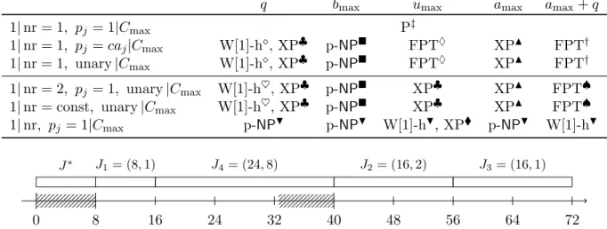
J^∗ J₁= (8,1) J₄= (24,8) J₂= (16,2) J₃= (16,1)

0 8 16 24 32 40 48 56 64 72

Figure 2: An example of the construction in the proof of Theorem 1 for an instance of Unary Bin Packing consisting of k = 2 bins each of size B = 4 and four objects o₁ to o₄ of sizes s1 = 1, s2 = s3 = 2, and s4 = 3. In the resulting instance of 1|nr = 1, pj = caj|C_max, there are five jobs (J^∗ and one job corresponding to each input object) and at each (whole) point in time of the hatched periods there is a supply of one resource. An optimal schedule that first schedules J^∗ is depicted. Note that the time periods between the (right-hand) ends of hatched periods correspond to a multiple of the bin size and a schedule is gapless if and only if the objects corresponding to jobs scheduled between the ends of two consecutive shaded areas exactly fill a bin.

In the following theorem, we show that even if each supply comes with a single unit of a resource, then the problem is already NP-hard.

Theorem 1. 1|nr = 1, pj =caj|C_maxis para-NP-hard with respect to the maximum numberbmax

of resources supplied at once even if all numbers are encoded in unary.

Proof. Given an instance I of Unary Bin Packing with Pn

i=1s_i = kB, we construct an instance I⁰ of 1|nr = 1|C_max with b_max= 1 as described below.

We define n jobs J1 = (p1, a1), J2 = (p2, a2), . . . , Jn = (pn, an) such that pi = 2Bsi and a_i = 2s_i. We also introduce a special job J^∗= (p^∗, a^∗), with p^∗ = 2B and a^∗= 1. Then, we set 2kB supply dates as follows. For eachi∈ {0,1, . . . , k−1}and x∈ {0,1, . . . ,2B−1}, we create a supply date q_i^x = (u^x_i,˜b^x_i) := ((2B+i2B²)−x,1). We add a special supply dateq^∗ := (0,1).

Next, we show that I is a yes-instance if and only if there is a gapless schedule for I⁰, that is,C_max= 2(B²+B). An example of this construction is depicted in Figure 2.

We first show that each solution toI can be efficiently transformed to a schedule withCmax= 2(B²+B). A yes-instance for I is a partition of the objects into k bins such that each bin is (exactly) full. Formally, there are k sets S₁, S₂, . . . S_k such that S

iS_i = O, S_i ∩S_j = ∅ for all i 6= j, and P

oi∈Sjsi = B for all j. We form a schedule for I⁰ as follows. First, we

(7)

schedule job J^∗ and then, continuously, all jobs corresponding to elements of set S1, S2, and so on. The special supply q^∗ guarantees that the resource requirement of job J^∗ is met at time 0. The remaining jobs, corresponding to elements of the partitions, are scheduled earliest at time 2B, when J^∗ is processed. The jobs representing each partition, by definition, require in total 2B resources and take, in total, 2B² time. Thus, it is enough to ensure that in each point 2B+i2B², for i∈ {0,1, . . . , k−1}, there are at least 2B resources available. This is true because for eachi∈ {0,1, . . . , k−1}the time point 2B+iB² is preceded with 2B−1 supplies of one resource. Furthermore, none of the preceding jobs can use the freshly supplied resources as the schedule must be gapless and all processing times are multiples of 2B. As a result, the schedule is feasible.

Now we show that a gapless schedule for I⁰ implies that I is a yes-instance. Let σ be a gapless schedule forI⁰. Observe that all processing times are multiples of 2B and therefore each job has to start at a time that is a multiple of 2B. For each i ∈ {0,1, . . . , k−1}, we show that there is no job that is scheduled to start before 2B +iB² and to end after this time. We show this by induction on i. Since at time 0 there is only one resource available, job J^∗ (with processing time 2B) must be scheduled first. Hence the statement holds for i = 0. Assuming that the statement holds for all i < i⁰ for some i⁰, we show that it also holds for i⁰. Assume towards a contradiction that there is a jobJ that starts before t := 2B+i⁰B² and ends after this time. LetS be the set of all jobs that were scheduled to start betweent0 := 2B+ (i⁰−1)B² and t. Recall that for each job J_j⁰ ∈S, we have that p_j⁰ =a_j⁰B. Hence, since J ends after t, the number of resources used by S is larger than ^(t−t⁰⁾/B = B. Since only 2B resources are available at timet, job J cannot be scheduled before time tor there is a gap in the schedule, a contradiction. Hence, there is no job that starts before t and ends after it. Thus, the jobs can be partitioned into “phases,” that is, there are k+ 1 sets T₀, T₁, . . . , T_k such that T₀ = {J^∗}, S

h>0Th =J \ {J^∗},Th∩Tj =∅for allh6=j, andP

Jj∈Tgpj = 2B² for allg. This corresponds to a bin packing whereog belongs to binh >0 if and only ifJg ∈T_h.

Note that Theorem 1 excludes pseudo-polynomial algorithms for the case under consideration since the theorem statement is true also when all numbers are encoded in unary. Theorem 1 motivates to study further problem-specific parameters. Observe that in the reduction presented in the proof of Theorem 1, we used an unbounded number of supply dates. Gy¨orgyi and Kis [23]

have shown a pseudo-polynomial algorithm for 1|nr = 1|C_max for the case that the number q of supplies is a constant. Thus, the question arises whether we can even obtain fixed-parameter tractability for our problem by taking the number of supply dates as a parameter. Devising a reduction from Unary Bin Packing, we answer this question negatively in the following theorem.

Theorem 2. 1|nr = 1, p_j =a_j|C_maxparameterized by the numberq of supply dates isW[1]-hard even if all numbers are encoded in unary.

Proof. We reduce from Unary Bin Packingparameterized by the number k of bins, which is known to be W[1]-hard [35]. Given an instanceI of Unary Bin Packingwith kbins, each of sizeB and nobjects o1, o2, . . . on of sizes1, s2, . . . sn such that Pn

i=1si =kB, we construct an instance I⁰ of 1|nr = 1|C_max as follows. We denote the set of all objects by O.

First, for each object oi ∈O, we define a job Ji = (pi, ai) such that pi =ai =si; we denote the set of all jobs by J. Next, we construct k supply dates qi = (ui,˜bi), with ui = (i−1)B and ˜b_i=B for each i∈[k]. This way we obtain an instance I⁰ of 1|nr = 1|C_max.

(8)

It remains to show that I is a yes-instance if and only ifI⁰ is an instance with Cmax =kB. To this end, suppose first that I is a yes-instance. Then, there is a partition of the objects into k bins such that each bin is (exactly) full. Formally, there are k sets S1, S2, . . . Sk such that S

iSi = O, Si ∩Sj = ∅ for all i 6= j, and P

oi∈S_jsi = B for all j. Hence we schedule all jobs j_i with o_i ∈ S₁ between time 0 = u₁ and B =u₂. Following the same procedure, we schedule all jobs corresponding to objects in Si between time ui and ui+1 where ui+1 = iB.

Since Pn

i=1pi =kB, we conclude that Cmax=kB.

Now suppose that C_max = kB. Assume towards a contradiction that there is an optimal schedule in which some jobJ_i ∈ J starts at some timetsuch thatt < u_` < t+p_ifor some`∈[k].

LetS be the set of all objects that are scheduled beforeJi. SinceCmax=kB, it follows that at each point of time until t, there is some job scheduled at this time. Thus, sincep_h =a_h for all jobsJ_h, it follows thatP

J_h∈Sa_h =P

J_h∈Sp_h =t. As a result,P

J_h∈S∪{Ji}a_h =t+a_i =t+p_i>

u` = (`−1)B = P`−1

h=1˜bh; a contradiction to ji starting before u`. Hence, there is no job that starts before someu_` and ends after it. Thus, the jobs can be partitioned into “phases,” that is, there areksetsT₁, T₂, . . . , T_ksuch thatS

hT_h =J,T_i∩T_i⁰ =∅for alli6=i⁰, andP

Jh∈T_gp_h =B for allg. This corresponds to a bin packing whereog belongs to binhif and only if Jg∈Th.

The theorems presented in this section show that our problem is (presumably) not fixed- parameter tractable either with respect to the number of supply dates or with respect to the maximum number of resources per supply. However, as we show in the following section, combining these two parameters allows for fixed-parameter tractability. Furthermore, we present other algorithms that, partially, allow us to successfully bypass the hardness presented above.

3 (Parameterized) Tractability

Our search for efficient algorithms forMaterial Consumption Scheduling Problemstarts with an introductory part presenting two lemmata exploiting structural properties of problem solutions. Afterwards, we employ the lemmata and provide several tractability results, including polynomial-time solvability for one specific case.

3.1 Identifying Structured Solutions

A solution to theMaterial Consumption Scheduling Problemis an ordered list of jobs to be executed on the machine(s). Additionally, the jobs need to be associated with their starting times. The starting times have to be chosen in such a way that no job starts when the machine is still processing another scheduled job and that each job requirement is met at the moment of starting the job. We show that, in fact, given an order of jobs, one can always compute the times of starting the jobs minimizing the makespan in polynomial time. Formally, we present in Lemma 1 a polynomial-time Turing reduction from 1|nr = r|C_max to 1,NI|nr = r|−. The crux of this lemma is to observe that there always exists an optimal solution to 1|nr =r|C_max that is decomposable into two parts. First, when the machine is idling, and second, when the machine is continuously busy until all jobs are processed.

Lemma 1. There is a polynomial-time Turing reduction from1|nr =r|C_max to1,NI|nr=r|−.

Proof. Assuming that we have an oracle for 1,NI|nr = r|−, we describe an algorithm solving 1|nr =r|C_max that runs in polynomial time.

(9)

We first make a useful observation about feasible solutions to the original problem. Let us consider some feasible solution σ to 1|nr = r|C_max and let g₁, g₂, . . . , g_n be the idle times before processing, respectively, the jobs J1, J2, . . . , Jn. Then, σ can be transformed to another schedule σ⁰ with the same makespan as σ and with idle times g⁰₁, g⁰₂, . . . , g_n⁰ such that g₂⁰ = g⁰₃. . . g_n⁰ = 0 and g₁⁰ =P

t∈[n]g_t. Intuitively, σ⁰ is a scheduling in which the idle times of σ are all “moved” before the machine starts the first scheduled job. It is straightforward to see that inσ⁰ no jobs are overlapping. Furthermore, each job according toσ⁰ is processed at earliest at the same time as it is processed according toσ. Thus, because there are no “negative” supplies and the order of processed jobs is the same in bothσ and σ⁰, each job’s resource request is met in scheduling σ⁰.

Using the above observation, the algorithm solving 1|nr = r|C_max using an oracle for 1,NI|nr = r|− problem works as follows. First, it guesses a starting gap’s duration g ≤u_max and then calls an oracle for 1,NI|nr =r|−subtractinggfrom each supply time (and merging all non-positive supply times to a new one arriving at time zero) of the original 1|nr =r|C_max instance. For each value ofg, the algorithm addsgto the oracle’s output and returns the minimum over all these sums.

Basically, the algorithm finds a scheduling with the smallest possible makespan assuming that the idle time happens only before the first scheduled job is processed. Note that this assumption can always be satisfied by the initial observation. Because of the monotonicity of the makespan with respect to the initial idle time g, the algorithm can perform binary search while searching forg and thus its running time isO(log(u_max)).

Let us further explain the crucial observation backing Lemma 1 since we will extend it in the subsequent Lemma 2. Assume that, for some instance of theMaterial Consumption Scheduling Problem, there is some optimal schedule where some jobJ starts being processed at some timet(in particular, the resource requirements ofJ are met att). If, directly after the job the machine idles for some time, then we can postpone processing J to the latest moment which still guarantees that J is ended before the next job is processed. Naturally, at the new starting time ofJ we can only have more resources than at the old starting time. Applying this observation exhaustively produces a solution that is clearly separated into idling time and busy time.

We will now further exploit the above observation beyond only “moving” jobs without chang- ing their mutual order. We first define adomination relation over jobs; intuitively, a job dominates another job if it is not shorter and at the same time it requires not more resources.

Definition 1. A job J_j dominates a job J_j⁰ (written J_j ≤_D J_j⁰) if p_j ≥p_j⁰ and a_i,j ≤a_i,j⁰ for all i∈ R.

When we deal with non-idling schedules, for a pair of jobsJj andJj⁰ whereJj dominatesJj⁰, it is better (or at least not worse) to scheduleJj beforeJ_j⁰. Indeed, since among these two, Jj’s requirements are not greater and its processing time is not smaller, surely after the machine stops processing Jj there will be at least as many resources available as if the machine had processedJ_j⁰. We formalize this observation in the following lemma.

Lemma 2. For an instance of 1,NI|nr|−, let <D be an asymmetric subrelation of≤_D. There always is a feasible schedule where for every pair Jj and J_j⁰ of jobs it holds that if Jj <_D J_j⁰, thenJ_j is processed before J_j⁰.

(10)

Proof. Letσ be some feasible schedule. Consider a pair (Jj, J_j⁰) of jobs such thatJj is scheduled afterJ_j⁰ andJ_j dominatesJ_j⁰, that is,p_j ≥p_j⁰,a_ij ≤a_ij⁰ for alli∈ R. Denote byσ⁰ a schedule emerging from continuously scheduling all jobs in the same order as in σ but with jobs Jj

and J_j⁰ swapped. Assume that σ⁰ is not a feasible schedule. We show that each job in σ⁰ meets its resource requirements, thus contradicting the assumption and proving the lemma. We distinguish between the set of jobsJ_out that are scheduled beforeJj⁰ inσ or that are scheduled afterJj inσ and jobsJ_inthat are scheduled betweenj⁰ andjinσ (includingj⁰ andj). Observe that since all jobs inJ_in are scheduled without the machine idling, it holds that all jobs inJ_out are scheduled exactly at the same times in bothσ and σ⁰. Additionally, since the total number of resources consumed by jobs inJ_in in bothσ andσ⁰ is the same, the resource requirements for each job inJ_out is met inσ⁰. It remains to show that the requirements of all jobs in J_inare still met after swapping. To this end, observe that all jobs except forJ_j⁰ still meet the requirements inσ⁰ asJj dominatesJ_j⁰ (i.e.,Jj requires at most as many resources and has at least the same processing time as J_j⁰). Thus, each job in J_in except for J_j⁰ has at least as many resources available inσ⁰ as they have inσ. Observe thatJ_j⁰ is scheduled later inσ⁰ thanJ_j was scheduled inσ. Hence, there are also enough resources available inσ⁰ to process J_j⁰. Thus, σ⁰ is feasible, a contradiction.

Note that in the case of two jobsJj andJ_j⁰ dominating each other (Jj ≤_D J_j⁰ andJ_j⁰ ≤_D Jj), Lemma 2 allows for either of them to be processed before the other one.

3.2 Applying Structured Solutions

We start with polynomial-time algorithms that applies both Lemma 1 and Lemma 2 to solve special cases of theMaterial Consumption Scheduling Problemwhere each two jobs can be compared according to the domination relation (Definition 1). Recall that if this is the case, then Lemma 2 almost exactly specifies the order in which the jobs should be scheduled.

Proof. We first show how to solve 1,NI|nr = 1, p_j = 1|−. At the beginning, we order the jobs increasingly with respect to their requirements of the resource arbitrarily ordering jobs with equal requirements. Then, we simply check whether scheduling the jobs in the computed order yields a feasible schedule, that is, whether the resource requirement of each job is met.

If the check fails, then we return “no,” otherwise we report “yes.” The algorithm is correct due to Lemma 2 which, adapted to our case, says that there must exist an optimal schedule in which jobs with smaller resource requirements are always processed before jobs with bigger requirements. It is straightforward to see that the presented algorithm runs inO(nlogn) time.

To extend the algorithm to 1|nr = 1, pj = 1|C_max, we apply Lemma 1. As described in detail in the proof of Lemma 1, we first guess the idling-timeg of the machine at the beginning.

Then, we run the algorithm for 1,NI|nr = 1, pj = 1|− pretending that we start at time g by shifting backwards by g the times of all resource supplies. Since we can guess g using binary search in a range from 0 to the time of the last supply, such an adaptation yields a multiplicative

1A weak order of elements ranks elements such that each two objects are comparable but different objects can be tied.

(11)

factor of O(logumax) for the running time of the algorithm for 1,NI|nr = 1, pj = 1|−. The correctness of the algorithm follows immediately from the proof of Lemma 1.

The aforementioned algorithms need only a small modification to work for the cases of 1|nr|−

and 1|nr|C_maxin which the domination relation is a weak order on a set of jobs. Namely, instead of sorting the jobs, one needs to find a weak order over the jobs. This is doable in quadratic time by comparing all pairs of jobs followed by checking whether the comparisons induce a weak order; thus we obtain the claimed running time. The obtained algorithm is correct by the same argument as the other above-mentioned cases.

Importantly, it is simple (requiring at most O(n²) comparisons) to identify the cases for which the above algorithm can be applied successfully.

If the given jobs cannot be weakly ordered by domination, then the problem becomes NP- hard as shown in Theorem 1. This is to be expected since when jobs appear which are in- comparable with respect to domination, then one cannot efficiently decide which job, out of two, to schedule first: the one which requires fewer resource units but has a shorter processing time, or the one that requires more resource units but has a longer processing time. Indeed, it could be the case that sometimes one may want to schedule a shorter job with lower resource consumption to save resources for later, or sometimes it is better to run a long job consum- ing, for example, all resources knowing that soon there will be another supply with sufficient resource units. Since NP-hardness probably excludes polynomial-time solvability, we turn to a parameterized complexity analysis to get around the intractability.

The time u_max of the last supply seems a promising parameter. We show that it yields fixed-parameter tractability. Intuitively, we demonstrate that the problem is tractable when the time until all resources are available is short.

Theorem 4. 1,NI|nr = 1|C_max parameterized by the time umax of the last supply is fixed- parameter tractable and can be solved in O(2^u^max·n+nlogn) time.

Proof. We first sort all jobs by their processing time in O(n) time using bucket sort. We then sort all jobs with the same processing time by their resource requirement in overall O(nlogn) time. We then iterate over all subsetsR of{1,2, . . . , u_max}. We will refer to the elements in R by r₁, r₂, . . . , r_k, where k = |R| and r_i < r_j for all i < j. For simplicity, we will use r₀ = 0.

For eachri in ascending order, we check whether there is a job with a processing time ri−ri−1

that was not scheduled before and if so, then we schedule the respective job that is first in each bucket (the job with the lowest resource requirement). Next, we check whether there is a job left that can be scheduled at rk and which has a processing time at least umax−rk. Finally, we schedule all remaining jobs in an arbitrary order and check whether the total number of resources suffices to run all jobs.

We will now prove that there is a valid gapless schedule if and only if all of these checks are met. Notice that if all checks are met, then our algorithm provides a valid gapless schedule. Now assume that there is a valid gapless schedule. We will show that our algorithm finds a (possibly different) valid gapless schedule. Let, without loss of generality, Jj1, Jj2, . . . , Jjn be a valid gapless schedule and let j_k be the index of the last job that is scheduled latest at time umax. We now focus on the iteration where R = {0, p_j₁, p_j₁ +p_j₂, . . . ,Pk

i=1p_j_i}. If the algorithm schedules the jobsJj1, Jj2, . . . , Jjk, then it computes a valid gapless schedule and all checks are met. Otherwise, it schedules some jobs differently but, by construction, it always schedules a

(12)

job with processing time pji at position i≤k. Due to Lemma 2 the schedule computed by the algorithm is also valid. Thus the algorithm computes a valid gapless schedule and all checks are met.

It remains to analyze the running time. The sorting steps in the beginning take O(nlogn) time. There are 2^u^max iterations forR, each takingO(n) time. Indeed, we can check in constant time for eachriwhich job to schedule and this check is done at mostntimes (as afterwards there is no job left to schedule). Searching for the job that is scheduled at time r_k also takes O(n) time as we can iterate over all remaining jobs and check in constant time whether it fulfills both requirements.

Another possibility for fixed-parameter tractability via parameters measuring the resource supply structure comes from combining the parametersq and b_max. Although both parameters alone yield intractability, combining them gives fixed-parameter tractability in an almost trivial way: By Assumption 1, every job requires at least one resource, sobmax·q is an upper bound for the number of jobs. Hence, with this parameter combination, we can try out all possible schedules without idling (which by Lemma 1 extends to solving to 1,NI|nr = 1|C_max).

Motivated by this, we replace the parameterbmaxby the presumably much smaller (and hence practically more useful) parametera_max. We consider scenarios with only few resource supplies and jobs that require only small units of resources as practically relevant. Next, Theorem 5 employs the technique of Mixed Integer Linear Programming (MILP) [8] to positively answer the question of fixed-parameter tractability for the combined parameter q+a_max.

Theorem 5.1,NI|nr = 1|C_maxis fixed-parameter tractable for the combined parameterq+a_max, where q is the number of supplies andamax is the maximum resource requirement per job.

Proof. Applying the famous theorem of Lenstra [39], we describe an integer linear program that uses only f(q, a_max) integer variables. Lenstra [39] showed that an (mixed) integer linear program is fixed-parameter tractable when parameterized by the number of integer variables (see also Frank and Tardos [18] and Kannan [36] for later asymptotic running-time improvements).

To significantly simplify the description of the integer program, we use an extension to integer linear programs that allows concave transformations on variables [8].

Our approach is based on two main observations. First, by Lemma 2 we can assume that there is always an optimal schedule that is consistent with the domination order. Second, within a phase (between two resource supplies), every job can be arbitrarily reordered. Roughly speaking, a solution can be fully characterized by the number of jobs that have been started for each phase and each resource requirement.

We use the following non-negative integer variables:

1. xw,s denoting the number of jobs requiring sresources started in phasew,

2. x^Σ_w,s denoting the number of jobs requiring s resources started in all phases between 1 and w(inclusive),

3. α_w denoting the number of resources available in the beginning of phasew,

4. d_w denoting the endpoint of phasew, that is, the time when the last job started in phasew ends.

Naturally, the objective is to minimizedq. First, we ensure thatx^Σ_w,sare correctly computed fromxw,sby requiringx^Σ_w,s=Pw

w⁰=1x_w⁰_,s.Second, we ensure that all jobs are scheduled at some

(13)

point. To this end, using #sto denote the number of jobs Jj with resource requirementaj =s, we add: ∀s∈[a_max] :P

w∈[q]x_w,s= #_s.Third, we ensure that theα_wvariables are set correctly, by settingα1= ˜b1, and∀2≤w≤q:αw =αw−1+˜bw−P

s∈[amax]xw−1,s·s.Fourth, we ensure that we always have enough resources: ∀2≤w≤q:α_w≥˜b_w.Next, we compute the endpointsd_w of each phase, assuming a schedule respecting the domination order. To this end, let p^s₁, p^s₂, . . ., p^s_#

s denote the processing times of jobs with resource requirement exactly s in non-increasing order. Further, let τ_s(y) denote the processing time spent to schedule the y longest jobs with resource requirement exactly s, that is, we have τs(y) = Py

i=1p^s_i. Clearly, τs(x) is a concave function that can be precomputed for each s∈[amax]. To compute the endpoints, we add:

∀w∈[q] :d_w = X

s∈[amax]

τ_s(x^Σ_w,s). (1)

Since we assume gapless schedules, we ensure that there is no gap: ∀1 ≤w ≤q−1 :dw ≥ u_w+1−1.This completes the construction of the mixed ILP using concave transformations. The number of integer variables used in the ILP is 2q·amax (for x^(Σ)w,s variables) plus 2q (q for αw

andd_w variables, respectively). Moreover, the only concave transformations used in Constraint Set (1) are piecewise linear with only a polynomial number of pieces (in fact, the number of pieces is at most the number of jobs), as required to obtain fixed-parameter tractability of this extended class of ILPs [8, Theorem 2].

4 A Glimpse on Multiple Resources

So far we focused on scenarios with only one non-renewable resource. In this section, we provide an outlook on scenarios with multiple resources (still considering only one machine). Natu- rally, all hardness results transfer. For the tractability results, we identify several cases where tractability extends in some form, while other cases become significantly harder.

Motivated by Theorem 5, we are interested in the computational complexity of theMaterial Consumption Scheduling Problem for cases where only amax is small. When nr = 1 anda_max= 1, then we have polynomial-time solvability via Theorem 3. The next theorem shows that this extends to the case of constant values of nr anda_maxif we assume unary encoding. To obtain this results, we develop a dynamic-programming-based algorithm for 1,NI|nr= 1|−and apply Lemma 1.

Theorem 6. 1|nr = const,unary|C_max can be solved in O(q·a^O(1)max ·n^O(a^max⁾·logu_max) time.

Proof. We will describe a dynamic-programming procedure that computes whether there exists a gapless schedule (Lemma 1). Letrbe the (constant) number of different resources. We distinguish jobs by their processing time as well as their resource requirements. To this end, we define the type of a job J_j as a vector (a_1,j, a_2,j,· · · , a_r,j)^T containing all its resource requirements.

LetT ={t₁, t₂, . . . , t_{|T |}}be the set of all types such that for allt∈ T there is at least one jobJ_j of typet. Let s:=|T | and note that s≤(amax+ 1)^r. We first sort all jobs by their type using bucket sort inO(n) time and then sort each of the buckets with respect to the processing times inO(nlogn) time using merge sort. For the sake of simplicity, we will use P_t[k] to describe the set of the k longest jobs of type t. We next define the`^th phase as the time interval from the start of any possible schedule up tou_`+1. Next, we present a dynamic program

T: [q]×[nt1]∪ {0} ×. . .×[nts]∪ {0} → {true, f alse},

(14)

wherenti is the number of jobs of typeti. We want to store trueinT[i, x1, . . . , xs] if and only if it is possible to schedule at least the jobs in P_t_k[x_k] such that all of these jobs start within thei^th phase and there is no gap. IfT[q, nt1, . . . , nts] is true, then this corresponds to a gapless schedule of all jobs and hence this is a solution. We will fill up the tableT by increasing values of the first argument. That is, we will first compute all entriesT[1, x₁, x₂, . . . , x_s] for all possible combinations of values forxi∈[nti]∪ {0}. For the first phase, observe thatT[1, x1, x2, . . . , xs] is set to true if and only if the two following conditions are met. First, there are enough resources available at the start to schedule all jobs in allP_t_i[x_i]. Second, the sum of all processing times of all “selected jobs” without the longest one end at least one time steps before u₂ (such that the job with the longest processing time can then be started at last in time stepu2−1 which is the last time step in the first phase). For increasing values of the first argument, we do the following to computeT[i, x₁, x₂, . . . x_s]. We compute for all tuples of numbers (y₁, y₂, . . . y_s) with y_k≤x_k for all k ∈ [s] whether T[i−1, y1, y2, . . . , ys] is true, whether the corresponding schedule can be extended to a schedule for T[i, x₁, x₂, . . . , x_s], and whether all selected jobs except for the longest one can be finished at least two time steps before u_i+1 −1. Since the first check and third check are very simple, we focus on the second check. To this end, it is actually enough to check whether P

k∈[s]

P

j∈P_tk[yk]p_j ≥ u_i−1 since if this was not the case but there still was a gapless schedule, then we could add some other job to the (i−1)^st phase and since we iterate over all possible combinations of values ofyi, we would find this schedule in another iteration.

It remains to analyze the running time of this algorithm. First, the number of table entries inT is upper-bounded byq·Q

k∈[s](n_t_k+1)≤(q·(n+1)^s). For each table entryT[i, x₁, x₂, . . . , x_s], there are at mostQ

k∈[s](xk+ 1)≤Q

k∈[s](ntk+ 1)∈O((n+ 1)^s) possible tuples (y1, y2, . . . , ys) with y_k≤x_k for all k ∈ [s] and the three checks can be performed in O(s) time. Thus, the overall running time isO(q·s·(n+ 1)^2s)⊆O(q·(a_max+ 1)^r·(n+ 1)^2r(a^max⁺¹⁾) for computing a gapless schedule and by Lemma 1 the time for solving 1|nr = const,unary|C_max is in O(q· (amax+ 1)^r·(n+ 1)^2r(a^max⁺¹⁾·logumax).

The question whether 1|nr = const,unary|C_max is inFPTor W[1]-hard with respect toa_max remains open even for only a single resource.

We continue with showing that already with two resources and unit processing times of the jobs, the Material Consumption Scheduling Problem becomes computationally in- tractable, even when parameterized by the number of supply dates. Note that NP-hardness for 1|nr = 2, pj = 1|C_max can also be transferred from Grigoriev et al. [21, Theorem 4] (the statement is for a different optimization goal but the proof works).

Proposition 1. 1|nr = 2, pj = 1|C_maxisW[1]-hard when parameterized by the number of supply dates even if all numbers are encoded in unary.

Proof. Given an instance I of Unary Bin Packing with k bins, each of size B, and n objects o₁, o₂, . . . o_n of sizes s₁, s₂, . . . s_n such that Pn

i=1s_i = kB, we construct an instance I⁰ of 1|nr = 2, pj = 1|C_max as follows.

For each i ∈ [k], we add a supply qi = (ui,˜b1,i,˜b2,i) := ((i−1)B, B, B(B −1)); thus, we createksupply dates. For each objecto_i fori∈[n], we create anobject job j_i= (p_i, a_1,i, a_2,i) :=

(1, si, B −si). Additionally, we create kB −n dummy jobs; each of them having processing time 1, no requirement of the resources of the first type, and requiringB resources of the second type. We refer to the constructed instance asI⁰.

We show that I is a yes-instance if and only if there is a schedule for the constructed instanceI⁰ with makespan exactlykB. Clearly, ifI is a yes-instance, then there is ak-partition

(15)

of the objects to subsetsS1, S2, . . . , S_ksuch that for eachi∈k,P

oj∈S_isj =B. For some setSi, we schedule all jobs inS_i, one after another, starting at time (i−1)B. Then, in the second step, we schedule the remaining dummy jobs such that we obtain a gapless schedule σ. Naturally, since eachSi contains at most B objects, the object jobs are non-overlapping in σ. Since in the second step we have exactly kB−n jobs available (recall that n is the number of object jobs) σ is a gapless schedule with makespan exactly kB. To check the feasibility of σ, let us consider the first B time steps. Note that from time 0 to time |S₁|, the machine processes all object jobs representing objects fromS₁; from time |S₁|+ 1 toB it processes exactlyB− |S₁|dummy jobs. Thus, the number of used resources of type 1 is P

oj∈Sis_j =B, and the number of used resources of type 2 isP

oj∈S_i(B−sj) + (B− |S₁|)B =|S₁|B−B+B²− |S₁|B =B(B−1). As a result, at time B−1 there are no resources available, so we can apply the argument for the first B time steps to all followingk−1 periods of B time steps; we eventually obtain that σ is a feasible schedule.

For the reverse direction, let σ be a schedule with makespan kB for instance I⁰. We again consider the first B time steps. Let J_p be the set of exactly B jobs processed in this time.

LetA1 andA2 be the usage of the resource of, respectively, type 1 and type 2 by the jobs inJp. We denote by J_o ⊆J_p the object jobs within J_p. Then, A₁ := P

j∈J_oa_1,j +P

j∈J_p\J_oa_1,j. In fact, since each dummy job has no requirement of the resources of the first type, we have A₁= P

j∈Joa1,j. Moreover, there are only B resources of type 1 available in the first B time steps, so it is clear that A₁ ≤B. Using the fact that, for each job j_i, it holds thata_2,i=B−a_1,i, we obtain the following:

A2 := X

j∈Jo

a2,j+ X

j∈Jp\Jo

a2,j

=|J_o|B−A1+|J_p\Jo|B=B²−A1.

Using the above relation between A₁ and A₂, we show that A₁ = B. For the sake of contradiction, assumeA1 < B. Immediately, we obtain that A2 > B²−B =B(B−1), which is impossible since we only have B(B −1) resources of the second type in the first B time steps of schedule σ. Thus, since A₁ = B, we use exactly B resources of the first type and exactly (B−1)B resources of the second type in the firstB time steps ofσ. We can repeat the whole argument to all followingk−1 periods ofB time steps. Eventually, we obtain a solution toI by taking the objects corresponding to the object jobs scheduled in the subsequent periods ofB-time steps.

The reduction is clearly applicable in polynomial time and the number of supply dates is a function depending solely on the number of bins in the input instance of Unary Bin Packing.

Proposition 1 limits the hope for obtaining positive results for the general case with multiple resources. Still, when adding the number of different resources to the combined parameter, we can extend our fixed-parameter tractability result from Theorem 5. Since we expect the number of different resources to be rather small in real-world applications, we consider this result to be of practical interest.

Proposition 2. 1,NI|nr =r|C_max is fixed-parameter tractable for the parameter q+amax+r, where q is the number of supplies andamax is the maximum resource requirement of a job.